
Figure
1.
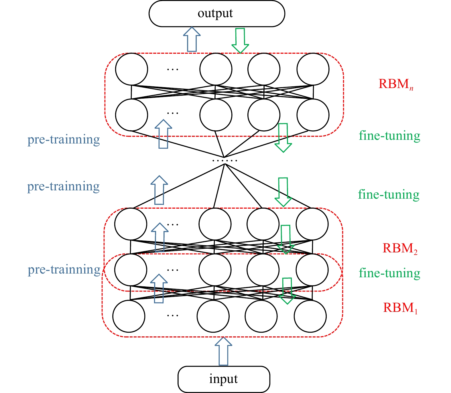
The deep belief network structure. RBM: restricted Boltzmann machine.
| Citation: | Yaojian Zhou, Yonglai Zhang, Wenai Song, Shijie Liu, Baoqiang Tian. A hybrid forecasting model for depth-averaged current velocities of underwater gliders[J]. Acta Oceanologica Sinica, 2022, 41(9): 182-191. doi: 10.1007/s13131-022-1994-4

|
Underwater gliders are excellent autonomous mobile ocean observation platforms (Webb et al., 2001; Eriksen et al., 2001; Sherman et al., 2001; Rudnick, 2016; Liu et al., 2020b). Compared with other platforms, underwater gliders have incomparable advantages such as low cost, long endurance, and convenient recovery. In recent years, they have been widely used in the observation of complex ocean phenomena such as air-sea interactions (Qiu et al., 2015) and mesoscale eddies (Qiu et al., 2019; Li et al., 2020) and achieved some significant results. However, buoyancy drive features make them highly sensitive to ocean currents, resulting in their failure to follow an arbitrary trajectory to a predetermined location (Rudnick et al., 2018). Therefore, it is essential to know the ocean flow information in advance in the environment where the glider will travel. However, being influenced by in situ observation capability, numerical ocean model forecast technology, and data storage technology, the existing ocean dynamics models for current forecasting possess many problems, such as low spatial resolution and a large number of errors, which means that the forecast values cannot satisfy the underwater glider application demand. Moreover, due to the limited carrying capacity and power, unless specifically required, underwater gliders are not equipped with current meters or acoustic Doppler current profilers (Zhou et al., 2017; Sun et al., 2020). Fortunately, the depth-averaged current (DAC) of underwater gliders can solve the above contradiction: the integration value of different types of ocean currents in glider profiles can be calculated directly by gliders rather than external current forecast models or ocean current sensors. The details of how to calculate the depth-averaged current velocity (DACV) can be seen in Zhou et al. (2017) and Merckelbach et al. (2008). Because DACV is an important and unique characteristic of underwater glider, its research is of great significance to the development of underwater glider. In particular, the study of DAC research can improve the ability of underwater gliders to perform observation missions and facilitate the development of other related ocean observation platforms.
Depth-averaged current velocities (DACVs) can be used to assist the navigation and path planning of underwater gliders in their deployments (Merckelbach et al., 2008; Chang et al., 2015). In addition, DACVs have many other applications, such as current equipment, and ocean model calibration. However, it is not easy to measure the DACV accurately, which depends on many factors, such as the pitch, measurement heading, and repeatable hydrodynamic shape (Rudnick et al., 2018).
In terms of actual utility, we care more about the predicted value of DACVs than its real-time measurement at most times because only the former can provide the glider with information about environmental currents in advance. However, compared with real-time measurement, predicting DACVs is even more challenging. Only a few scholars have studied DACVs prediction, and there are many limitations in their forecasting schemes. For example, Chang et al. (2015) divided the DACV into tidal components and nontidal components, and then the tidal component was forecasted by a tidal model. Additionally, the nontidal component was predicted by an empirical hybrid ocean model based on the experimental data collected by a glider, and the predicted DACVs consisted of the two predicted components. Similarly, Merckelbach et al. (2016) divided the DACV near the North Sea into a tidal component and a nontidal component, and then the two components were predicted by a Kalman filter based on the linear shallow water equation and the first-order Butterworth low-pass filter. Considering that these methods are only applicable to areas with significant tidal current components (e.g., offshore) and that special tidal models are needed in the calculation, these methods become impractical. Therefore, we proposed some DACV forecasting schemes without the need for particular models in the early stages. In our previous works, the DACVs were regarded as time series, similar to some recent literature (Zeiden et al., 2019; Kerfoot and Aragon, 2020). Then, four forecasting schemes were applied for the DACVs, among which empirical mode decomposition (EMD)-based methods showed inherent robustness and superiority (Zhou et al., 2017). In addition to EMD, hybrid methods based on decomposition have been widely accepted in time series prediction, which typically consists of data decomposition by methods such as ensemble empirical mode decomposition (EEMD) (Wang et al., 2015), complementary ensemble empirical mode decomposition (CEEMD) (Yang and Wang, 2018), and discrete wavelet transform (DWT) (Jiang et al., 2018; Bhardwaj et al., 2020). Among them, DWT showed superior forecasting performance (Jiang et al., 2018).
To improve the forecasting accuracy, this paper first utilizes DWT to decompose the DACV series. After decomposition, the original DACV series is divided into several subseries, which include the high-frequency components and the low-frequency component. Generally, high-frequency components often contain more randomness and uncertainty, whereas low-frequency components contain less randomness and uncertainty. Then, different forecasting models are established for the above two components. To capture the complex characteristics of DACV, a deep belief network (DBN) is applied for high-frequency component forecasting, which is a time-varying parameter model that can capture the dynamic variation in the high-frequency component. In addition to high-frequency component forecast, the least squares support vector machine (LSSVM) is used for low-frequency component forecasting. This is because LSSVM showed good forecasting performance for DACVs in our previous work (Zhou et al., 2017). The forecasting result of the origin series can be obtained by adding the forecasting results of each subseries. The innovations of this paper are as follows: the hybrid model is built according to the characteristics of different components. Therefore, the complicated characteristics of DACVs can be well captured, furthermore, the hybrid model based on DWT, DBN, and LSSVM is first proposed for DACV prediction, and compared with other models, and the robustness and effectiveness of the model are verified. The research results of this paper can provide critical support for the efficient operation of an underwater glider, provide a theoretical basis for the planning and precise navigation of underwater gliders, and lay a foundation for the study of ocean currents, sea breezes, waves, and other forecasting methods.
The remainder of this paper is organized as follows. In Section 2, DWT, DBN and LSSVM are briefly introduced, while the hybrid model is shown in detail. A case study is given in Section 3, in which the DACV data sources, evaluation criteria, and analysis of forecasting results are demonstrated. Based on the results of the above cases, we discussed them in Section 4, including the validity, sensitivity and further discussion. Conclusions are given in Section 5.
Wavelet transform (WT) is the best representative achievement in the field of applied mathematics, control engineering, and artificial intelligence. The discrete form of WT is DWT (discrete wavelet transform). As a popular decomposition technique, DWT is widely used in the decomposition and analysis of all kinds of data, especially for nonstationary and nonlinear data (Devi and Singh, 2020; Amin et al., 2020; Liu et al., 2020a). Similar to EMD, a given series X(t) can be decomposed into the following form:
| $$ X\left(t\right)=\sum _{i=1}^{m} {c}_{i}\left(t\right), $$ | (1) |
where ci(t) is the ith subseries, which represents the signal component of different feature scales of the original series X(t). m is the number of obtained subseries, and the first m − 1 subseries correspond to the detailed components, while the last subseries corresponds to the approximate component. The former can give the signal details, whereas the latter is used to represent the characteristics of the signal. In our research, the detailed components are regarded as the high-frequency components, while the approximate component is seen as the low-frequency component. m − 1 is also known as the number of decomposed layers. Different from EMD, m should be given in advance before DWT is adopted, and the form of wavelet bases needs to be identified ahead at the same time. More detail of the DWT can be seen in Bhardwaj et al. (2020) and Su et al. (2015).
The DBN is the earliest and representative deep learning network (Hinton et al., 2006), the structure of which is given in Fig. 1. DBN is often used in complex time series prediction with good results (Pan et al., 2020; Shi et al., 2021; Qiu et al., 2017). The DBN consists of several stacked restricted Boltzmann machines (RBMs), and each RBM unit is composed of a visible layer and a hidden layer. For the DBN, no connection exists in the same layer, but there are restricted complete connections in different layers. The DBN can capture the depth characteristics of data through a particular structure, which ensures its effective processing of nonlinear and high-dimensional data. Backpropagation (BP) and other traditional artificial neural networks have local minimization problems and lack adaptability, while the DBN can overcome these two shortcomings effectively. The DBN training process can be divided into two steps: pretraining and fine tuning.
The pretraining step is used to initialize the parameters of each RBM layer, and the parameters consist of weights and offsets. In the process of pretraining, the input of the first hidden layer is usually untagged data, and the output of the first hidden layer is regarded as the input of the second hidden layer. This process is repeated until the nth layer training is completed, and then the initialization parameters of each RBM can be obtained.
After preprocessing, each RBM can only ensure that its own layer output characteristics are the best, not the whole. To overcome the shortcoming that the parameters are easily trapped in the optimal local value, the DBN is optimized by sing the BP algorithm. Then, the parameters of the entire DBN are adjusted from the top-down and bottom-up, which is called the fine-tuning process.
In using DBN to predict DACVs, the input refers to the historical lag period DACVs, and the output refers to DACVs to be predicted. The prediction in this paper only refers to one-step prediction, and the prediction steps are the same as those of using BP neural network (Zhou et al., 2017).
The form of the LSSVM model is as follows (Zhang and Wang, 2006):
| $$ \mathbf{{\boldsymbol{y}}}\left(\mathbf{{\boldsymbol{x}}},K\right)=\sum _{i=1}^{K} {\mathit{{\boldsymbol{a}}}}_{i}\left(K\right)k\left(\mathbf{{\boldsymbol{x}}},{\mathbf{{\boldsymbol{x}}}}_{i}\right)+\mathit{{\boldsymbol{b}}}, $$ | (2) |
where
As a kind of complex spatiotemporal data in nature, DACV is the synthesis of ocean currents at different time and space positions in the profile of an underwater glider, whereas the composition of ocean currents is rather complex (Goldstein et al., 1989; Neumann, 2014). Moreover, due to the limited endurance of underwater gliders, the number of successive gliding profiles is limited, so the DACV samples obtained by the underwater glider during a continuous voyage are also limited. In the actual operation of underwater gliders, 1 000 m is a typical set depth. At this depth, it usually takes 2–4 h for a profile. The number of continuous profiles of domestic underwater gliders usually does not exceed 500, which corresponds to the endurance of no more than three months. For DACV data with complex characteristics and limited sample size, even if we regard it as a time series, it still has great uncertainty and randomness, and DACV prediction is even harder.
In order to predict DACV with high precision, the effect of a single prediction method may be limited. The reasonable idea is to decompose the original sequence into several simpler sub-sequences, and then predict each sub-sequence with the same prediction tool, and finally add the prediction results of each sub-sequence, which is exactly corresponding to our previous works (Zhou et al., 2017). Here, a more efficient DWT decomposition scheme is adopted to replace the previous EMD decomposition scheme, and the sub-sequence is no longer predicted by a single prediction tool but by two different prediction tools according to the different frequency characteristics. This hybrid method is DWT-DBN-LSSVM method proposed in this paper. This hybrid method is a purely data-driven prediction method without considering the internal mechanism. Meanwhile, this hybrid method can give full play to the advantages of each component, which is explained as follows:
(1) One of the motives of this paper is to decompose the natural discrete data of time series into components of different frequencies, and DWT perfectly caters to this motive. In addition, as mentioned in (Jiang et al., 2018), the hybrid forecasting method based on DWT decomposition is far better than the hybrid forecasting method based on EMD (or its derivative) decomposition, probably because the former has good localization characteristics in both the time domain and frequency domain.
(2) As an original deep learning tool (Hinton et al., 2006), compared with the conventional shallow models, DBN can express functions with high variance, discover the potential laws in multiple features, and achieve a better generalization capacity (Bengio, 2009; Sun et al., 2017). Compared with other deep learning tools (e.g., Long Short Term Memory (LSTM), Recurrent Neural Network (RNN), Gate Recurrent Unit (GRU)), DBN seems to perform better than LSTM, RNN and other new forecasting tools in some data predictions with small sample sizes (Wang et al., 2021). For the high-frequency part, DBN is adopted, which has deep learning ability and strong adaptability and can capture irregular trends.
(3) The shallow model LSSVM shows a superior effect in the prediction of small samples, which has been previously confirmed (Zhou et al., 2017). Compared with Autoregressive Integrated Moving Average Model, LSSVM can deal with nonlinear and nonstationary sequences with much faster computing speed. Therefore, the low-frequency part adopts LSSVM.
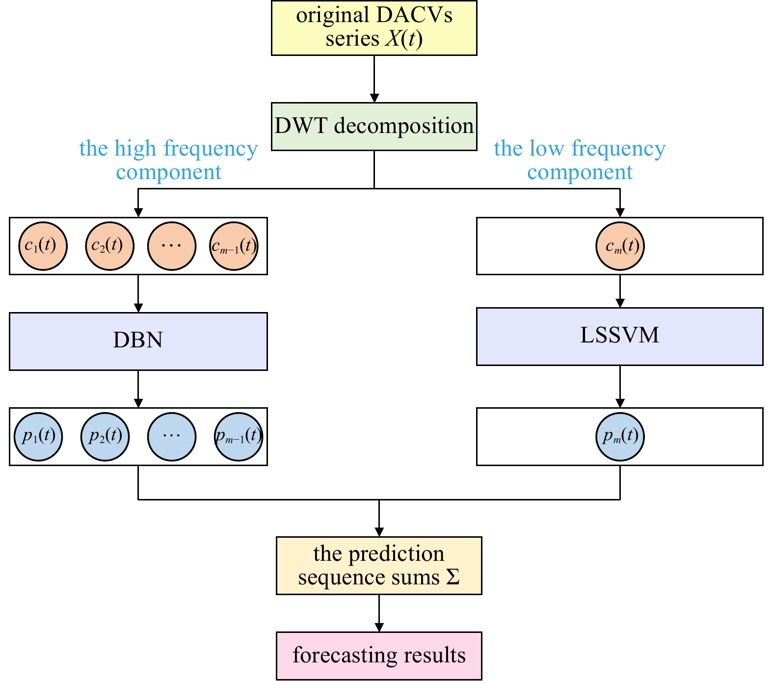
The hybrid model DWT-DBN-LSSVM is executed as follows. First, to better capture the complex characteristics, DWT decomposition is adopted. Through decomposition, the original DACV series is decomposed into several subseries. According to the criterion given in Section 2.1, the high- and low-frequency components can be determined. For the high-frequency part, DBN is used. For low-frequency part, LSSVM is utilized. Then, we can obtain the DACV forecasting results by summing the forecasting results of all the subseries. The structure of the hybrid model can be seen in Fig. 2.
It should be noted that the hybrid model used in this paper is DWT-DBN-LSSVM. If the components of each part are replaced, the prediction accuracy will be significantly affected (see Section 3.3.2 for details). At the same time, each component has its specific hyperparameters, such as the number of decomposition layers of DWT, wavelet basis, the number of RBM layers in DBN, the number of neurons contained in each layer and the lag order of DBN and LSSVM. These hyperparameters, which are confirmed in Section 3.3 and are tested for sensitivity in Section 4.2, also have a significant impact on prediction accuracy.
Two groups of DACVs from sea trials are utilized to test and verify the forecasting model. To better demonstrate the superiority of the proposed model, we first compare it with some well-recognized single forecasting models. To illustrate the superiority of each component in the proposed model, we then compare it with some hybrid models.
The two DACV datasets (465 DACVs from glider J019 and 488 DACVs from glider J021) are from sea trials of the same period, and the time of the sea trials is from middle July to late September 2019, the location of the sea trials is the South China Sea, which can be seen in Fig. 3. To make the figures clearer, the DACVs are sampled and drawn at an interval of 2. From Fig. 3, it can be seen that during this sea trial, both gliders J019 and J021 were sampled back and forth around a specified line, which was related to the specific mission at that time.
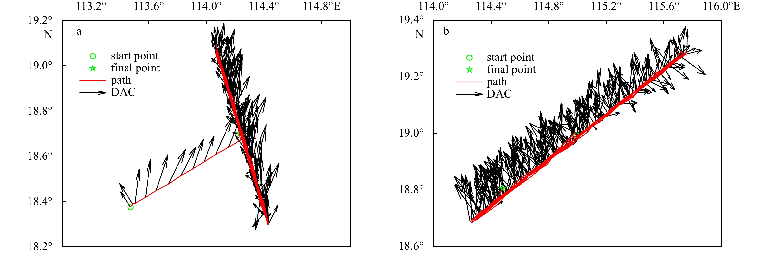
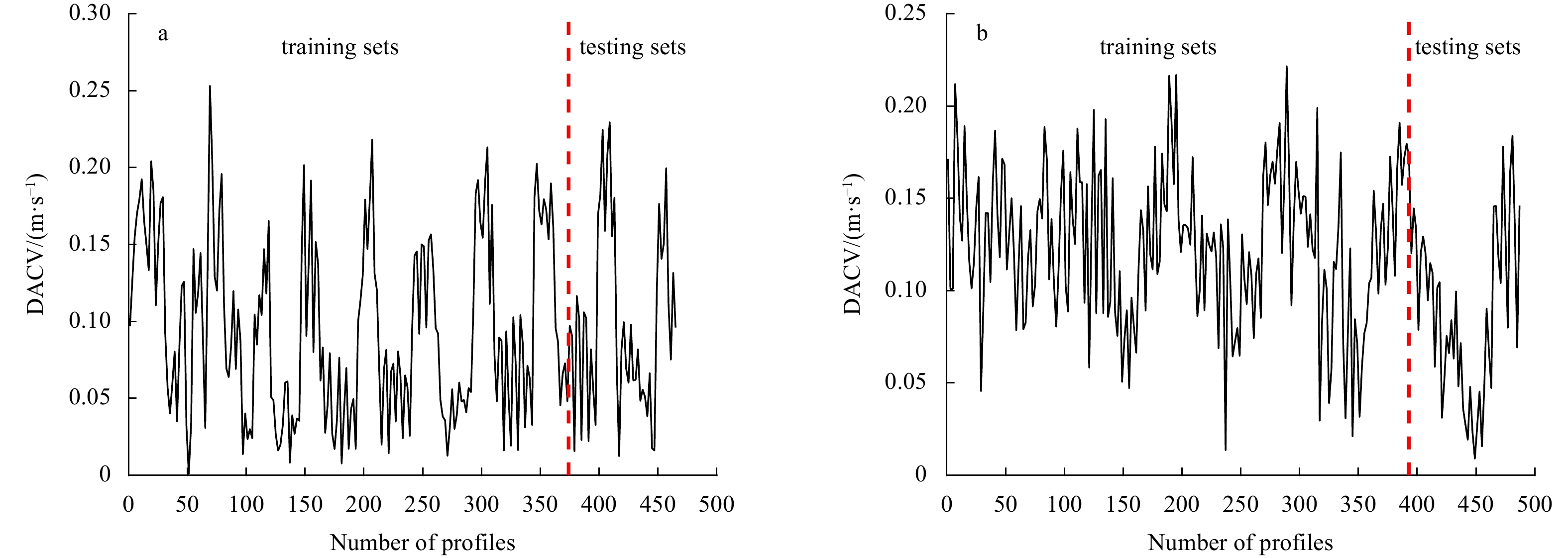
The corresponding depth of all profiles is 1 000 m, and the time cost of each profile is distributed between 3.5 h and 4.5 h, which depends on different settings, such as pitch angle and input net buoyancy. Although the underwater glider deploys in a three-dimensional ocean environment, the DACVs are only two-dimensional data: the DACV magnitude and the DACV direction. The DACV time series used in this research is simulated as the magnitude, which is similar to wind speed prediction in many existing studies (Song et al., 2018; Zhang et al., 2020).The magnitude of DACVs is drawn in Fig. 4, and the interval is set to 2 to be consistent with Fig. 3. The statistics for all DACV data are calculated and displayed in Table 1.
| Glider | Median/ (m·s−1) | Mean/ (m·s−1) | Max/ (m·s−1) | Min/ (m·s−1) | Std. |
| J019 | 0.083 2 | 0.094 8 | 0.277 2 | 0.001 0 | 0.0579 |
| J021 | 0.119 5 | 0.117 2 | 0.222 4 | 0.005 1 | 0.046 4 |
 DownLoad:
CSV
DownLoad:
CSV
Each data set is split into two parts: the training set and the testing set. The training set is used to build predictive models, and the test set is adopted to verify accuracy. The training set accounts for 80%, and the test set accounts for 20%, which is the same as many existing studies (Fan et al., 2008; Kilic et al., 2021).
Four commonly used error evaluation criteria, mean absolute error (MAE), mean absolute percentage error (MAPE), root mean square error (RMSE), and max absolute error (Max-AE), are adopted to evaluate the prediction effects of the different prediction models. They are calculated as follows:
| $$ \mathrm{M}\mathrm{A}\mathrm{E}=\frac{1}{N}\sum _{t=1}^{N} \left|X\left(t\right)-\widehat{X}\left(t\right)\right|, $$ | (3) |
| $$ \mathrm{M}\mathrm{A}\mathrm{P}\mathrm{E}=\frac{1}{N}\sum _{{t}=1}^{N}\left|\frac{X\left({t}\right)-\widehat{X}\left({t}\right)}{X\left({t}\right)}\right|, $$ | (4) |
| $$ \mathrm{R}\mathrm{M}\mathrm{S}\mathrm{E}=\sqrt{\frac{1}{N}\sum _{{t}=1}^{N}\frac{1}{N}\left[X\right({t})-\widehat{X}({t}){]}^{2}}, $$ | (5) |
| $$ {\mathrm{Max}}\text{-} \mathrm{A}\mathrm{E}=\mathrm {max}\left\{\left|X\left({t}\right)-\widehat{X}\left({t}\right)\right|\right\} \ \ \left({t}\in \left[1,N\right]\right), $$ | (6) |
where X(t) denotes the origin DACVs, and N is the number of the DACV samples of the X(t) series.
Even if the results of one prediction model are more accurate than one of another, it is not enough to guarantee that the former will perform better in all practical situations. In order to ensure that the prediction accuracy is stable, the significance of the prediction results should be tested for both models. Therefore, diebold-Mariano (DM) tests (Diebold and Mariano, 1995) can be used for this purpose. A detailed theory of the DM test is given below.
Step 1: Two hypotheses are given, which are called the original hypothesis H0: the disparities between the any two predicted errors are not obvious; and the alternative hypothesis H1 : the forecasting errors of the compared models are quite discrepant.
Step 2: The following formula is used to calculate the DM test statistics:
| $$ {S}_\mathrm{DM}=\frac{\bar{d}}{\sqrt{{\widehat{f}}_{\bar{d}}/T}}, $$ | (7) |
where
| $$ \hat{d}=\frac{1}{T}\sum _{{t}=1}^{T} \left[\mathrm {Loss}\left({d}_{{t}}^{1}\right)-\mathrm {Loss}\left({d}_{{t}}^{2}\right)\right], $$ | (8) |
where
Step 3: Given a significance level
As described in the proposed model above, the original DACVs are first decomposed into their components. The number of decomposition levels has considerable impacts on the prediction accuracy (Meng et al., 2016). There are problems if the quantity is too large or too small. For the former, some information in the original data may be distorted, and an illusive component may be introduced into the subseries, while for the latter, the nonstationary and nonlinear characteristics existing in the original data may not be effectively reduced. Through trial and tests, the number of levels is determined to be 9, and “db10” is adopted as the wavelet. For simplicity, we only demonstrate the decomposition of DACVs derived from J019, which is given in Fig. 5.

According to the criterion given in Section 2.1, for Fig. 5, C1 to C9 are seen as the high-frequency components, while C10 is regarded as the low-frequency component. Then, these high-frequency components can be forecasted by the DBN model, and we set the parameters as follows: the layers of RBMs L1=2, the number of neurons in each layer is set to 10, the activation function of the hidden layers is selected as “sigmoid”, and the activation function of the output layer is selected as “purelin”. The low-frequency component is predicted by the LSSVM model. Determined by trial and error, we set the DBN and LSSVM lag as 9. Next, we use the proposed forecasting model to forecast the above two DACV datasets. We first compare the results with some well-recognized single models, and then we compare the results with some related hybrid models to show the effectiveness of each part of the proposed model.
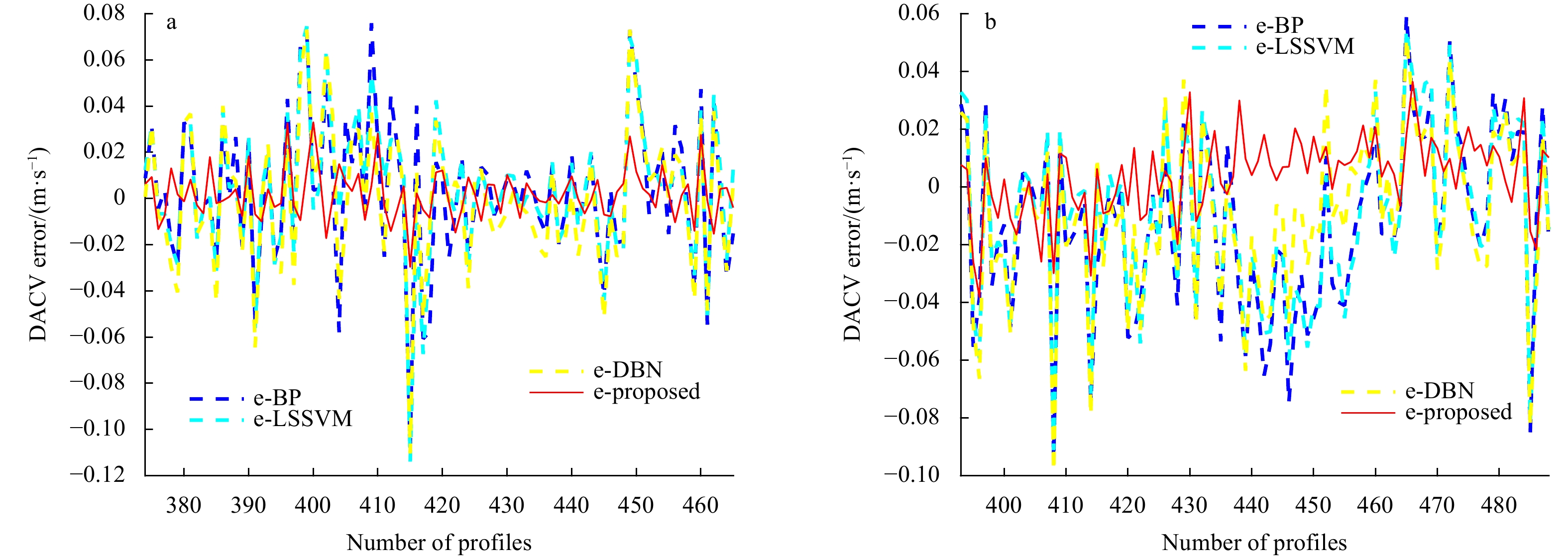
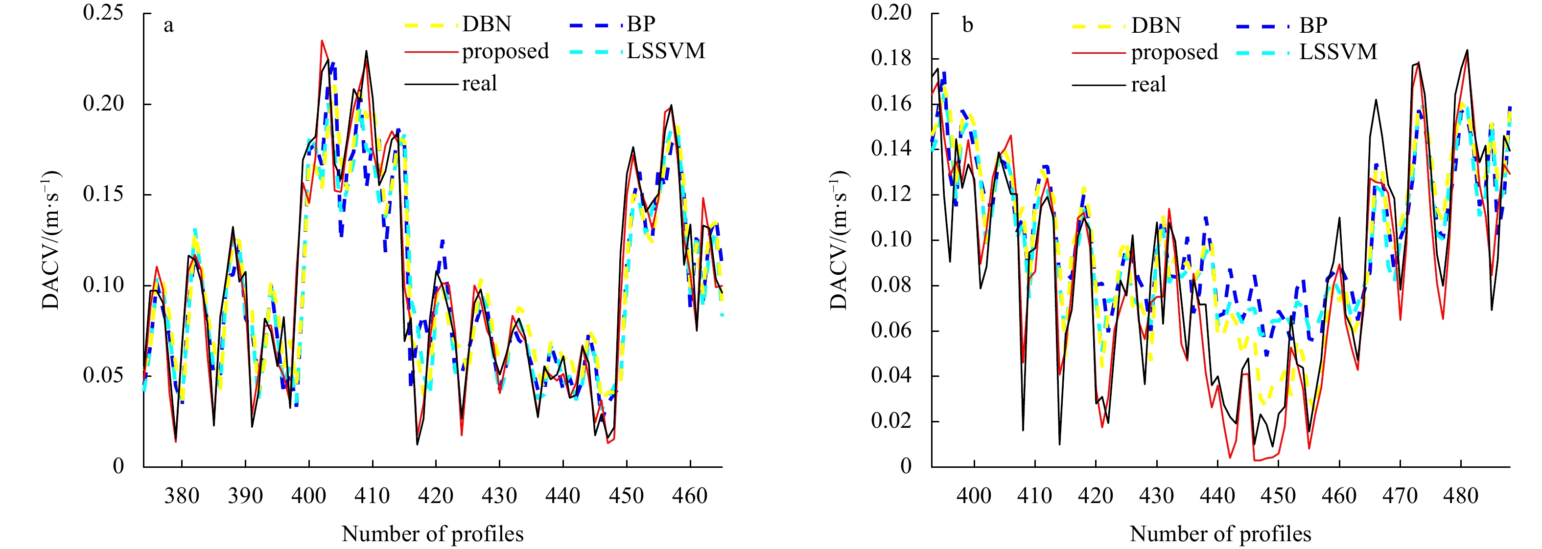
Because BP and LSSVM are adopted in our previous work (Zhou et al., 2017), DBN is the essential part of the proposed model. These three models are also well-recognized single models. Therefore, we use BP, LSSVM, and DBN as the comparison models. The profile forecasts of the DACVs from the two gliders are shown in Fig. 6, while the errors of the two are shown in Fig. 7. The comparison results of all models of the two DACVs are given in Tables 2 and 3. In Figs 6, 7 and Tables 2, 3, it can be found that the accuracy of the proposed model is far better than that of the single models. These results show that the hybrid model is superior to the single model in DACV prediction. The reason is that these single models cannot effectively capture the complex features of the original series, while the hybrid model combined with DWT, DBN and LSSVM can better capture the complex features of the original series. We can observe that the BP model has the largest MAE and RMSE which corresponds to its relatively poor predictive performance. Nevertheless, the Max-AE of the BP model is not the maximum. This indicates that compared with LSSVM and DBN, the fluctuation of BP prediction results is not that bad. Another interesting observation is that the MAPE of all the forecasting results with different models is not small. This is because the true DACV values of some profiles are small (near 0), while the forecasting errors of the same profiles have the same order of magnitude as the true values. For example, in Fig. 6a, the real value of the 417th profile is 0.012 4 m/s, while the error using LSSVM is −0.067 m/s for the same profile, which can be seen in Fig. 7a.

| J019 | BP | LSSVM | DBN | Proposed |
| MAE | 0.022 1 | 0.022 1 | 0.023 3 | 0.008 1 |
| MAPE/% | 39.98 | 39.01 | 42.42 | 10.53 |
| RMSE | 0.031 3 | 0.030 0 | 0.030 3 | 0.010 9 |
| Max-AE | 0.107 8 | 0.113 9 | 0.110 4 | 0.033 1 |
| CT/s | 0.560 0 | 5.88 | 2.03 | 21.7 |
| Note: BP represents back-propagation; LSSVM, least squares support vector machine; DBN, deep belief network. | ||||
DownLoad:
CSV
| J021 | BP | LSSVM | DBN | Proposed |
| MAE | 0.022 6 | 0.025 5 | 0.023 1 | 0.011 5 |
| MAPE/% | 74.37 | 70.30 | 57.36 | 23.22 |
| RMSE | 0.032 9 | 0.031 5 | 0.029 6 | 0.014 2 |
| Max-AE | 0.091 4 | 0.091 2 | 0.098 6 | 0.038 2 |
| CT/s | 1.62 | 112.0 | 4.68 | 52.5 |
| Note: BP represents back-propagation; LSSVM, least squares support vector machine; DBN, deep belief network. | ||||
DownLoad:
CSV
Computation time (CT) is another important indicator of the effectiveness of all algorithms, and it is also closely related to the timeliness of the prediction model in this paper. Therefore, we also provide the computation time of each prediction model in Tables 2 and3. It is important to point out that the computation time is dependent on the system environment. The computer we used was Lenovo ThinkPad P52s, corresponding to the processor: Intel(R)Core (TM)I7-8550U CPU@1.80GHZ(8 CPUS), m2.0GHZ. The operating system is Win10 64-bit system, while the prediction model was realized by Matlb2018b.
It can be seen that among the single algorithms, BP requires the lowest computation time, followed by DBN and LSSVM. The time of the proposed method is several times that of DBN/LSSVM because the time complexity of prediction for each of its subsequences is comparable to that of prediction for a single sequence (DBN or LSSVM). In spite of this, the time required by the proposed model calculation is still negligible compared with that required by a single underwater glider profile, which indicates that the proposed algorithm has good real-time prediction performance.
To further demonstrate the effectiveness of each part of the model proposed in this paper, two different experiments are carried out to verify the contribution of each part.
(1) Effectiveness of DWT
DWT is used for decomposing the origin DACVs. To validate the effectiveness of DWT, some other decomposition-based models are used for comparison, including EMD, EEMD, and CEEMD. The comparison results of EMD-DBN-LSSVM (Model 1), EEMD-DBN-LSSVM (Model 2), CEEMD-DBN-LSSVM (Model 3) and the proposed model are shown in Tables 4 and 5. In the two tables, we find that the MAE, MAPE, RMSE and Max-AE of the proposed model are smaller than those comparative models. Specifically, compared with Model 1, Model 2 and Model 3, the forecasting results of MAE for J019 are improved by 60.1%, 60.3%, and 60.5%; and the MAPE is reduced by 62.9%, 70.0%, and 62.8% ; the RMSE is decreased by 57.2%, 58.9%; and 56.1%, and the MaxAE is reduced by 50.0%, 62.0%, and 48.7%. This results show that compared with EMD-based (or its derivative) models, feature extraction is more effective by DWT. The reason for this is that because DWT has good localization characteristics in both the time domain and frequency domain.
| J019 | Model 1 | Model 2 | Model 3 | Proposed |
| MAE | 0.020 3 | 0.020 4 | 0.020 5 | 0.008 1 |
| MAPE/% | 28.36 | 35.14 | 28.27 | 10.53 |
| RMSE | 0.025 5 | 0.026 5 | 0.024 8 | 0.010 9 |
| Max-AE | 0.006 61 | 0.086 9 | 0.064 5 | 0.033 1 |
| CT/s | 17.4 | 18.2 | 19.2 | 21.67 |
DownLoad:
CSV
| J021 | Model 1 | Model 2 | Model 3 | Proposed |
| MAE | 0.023 4 | 0.020 7 | 0.022 2 | 0.011 5 |
| MAPE/% | 55.55 | 48.10 | 48.99 | 23.22 |
| RMSE | 0.027 8 | 0.025 0 | 0.026 6 | 0.014 2 |
| Max-AE | 0.069 2 | 0.066 7 | 0.066 7 | 0.038 2 |
| CT/s | 38.7 | 38.1 | 48.8 | 52.5 |
DownLoad:
CSV
In Tables 4 and 5, we can also see that compared with Models 1,2 and 3, the computation time of the proposed model is the longest, indicating that DWT decomposition takes more time than the other three kinds of decomposition.
(2) Effectiveness of DBN-LSSVM
For the proposed model, after DWT, DBN-LSSVM is the rest. To validate the effectiveness of this part, we fix DWT and replace DBN-LSSVM with different components related to it, including DBN, LSSVM, and LSSVM-DBN. Therefore, three comparison models DWT-DBN (Model 4), DWT-LSSVM (Model 5), and DWT-LSSVM-DBN (Model 6) are generated. Among them, DWT-DBN refers to the decomposition of DACVs by DWT first, then each sub-sequence is forecasted by DBN, and the DACV forecasting results are obtained by summing the forecasting results of all the subseries; DWT-LSSVM is similar to DWT-DBN, except that the predictor of subsequence is changed to LSSVM; DWT-LSSVM- LSSVM is similar to the model proposed in this paper, except that LSSVM is used for high-frequency subsequences while DBN is used for low-frequency subsequences. Comparison results are shown in Tables 6 and 7. As Tables 6 and 7 reveal, the values of the four error indexes all decrease. For example, comparing the proposed model with Model 4, Model 5 and Model 6, the RMSE for J019 decreases by 48.9%, 43.0%, and 46.5%, respectively. These results show that DBN is suitable for the prediction of high-frequency subseries, while LSSVM is suitable for forecasting low-frequency subseries. Once the subseries decomposed by DWT are laid out from high frequency to low, utilizing the combination of DBN-LSSVM for forecasting is better than using the DBN and LSSVM alone, and the combination of DBN-LSSVM is superior to the combination of LSSVM-DBN.
| J019 | Model 4 | Model 5 | Model 6 | Proposed |
| MAE | 0.012 9 | 0.010 9 | 0.015 3 | 0.008 1 |
| MAPE/% | 17.85 | 15.98 | 22.82 | 10.53 |
| RMSE | 0.017 0 | 0.014 3 | 0.019 0 | 0.010 9 |
| Max-AE | 0.058 3 | 0.050 0 | 0.050 0 | 0.033 1 |
| CT/s | 18.9 | 55.3 | 55.7 | 21.7 |
DownLoad:
CSV
| J021 | Model 4 | Model 5 | Model 6 | Proposed |
| MAE | 0.018 9 | 0.027 0 | 0.027 9 | 0.011 5 |
| MAPE/% | 39.47 | 62.66 | 64.58 | 23.22 |
| RMSE | 0.022 0 | 0.031 4 | 0.032 1 | 0.014 2 |
| Max-AE | 0.052 3 | 0.049 3 | 0.050 5 | 0.038 2 |
| CT/s | 43.2 | 141.8 | 135.0 | 52.5 |
DownLoad:
CSV
In Tables 6 and 7, we still give the computation time of each prediction model. It can be seen that Model 5 and Model 6 require longer computation time, while Model 4 requires the least, because LSSVM requires more computation time than DBN for subsequence. The computation time of the proposed model is slightly longer than that of Model 4, because 9 of the 10 subsequences of the proposed model are predicted by DBN, one is predicted by LSSVM, and all 10 subsequences of Model 4 are predicted by DBN.
This section discusses the validity and sensitivity of the proposed model, and further discusses the model performance boundary, applicable conditions and data characteristics of DACVs. These are discussed in the following subsections.
There are many criteria for model validity, and DM test is a widely used criterion. In the DM test, the null hypothesis describes that the predictive performance of the proposed model is as valid as that of the comparison model, while the alternative hypothesis means that the predictive performance of the proposed model is significantly different from that of other models. The average values of the DM test values from DACVs of J019 and J021 between the proposed model and other models are given in Table 8.
| Model | SDM |
| BP | 5.307 6 |
| LSSVM | 6.284 2 |
| DBN | 7.690 2 |
| Model 1 | 7.996 3 |
| Model 2 | 5.080 7 |
| Model 3 | 5.332 7 |
| Model 4 | 2.876 5 |
| Model 5 | 3.466 9 |
| Model 6 | 3.256 1 |
| Note: BP represents back-propagation; LSSVM, least squares support vector machine; DBN, deep belief network. | |
DownLoad:
CSV
Table 8 clearly shows that the smallest value of DM test is 2.876 5, which is outside [−2.58+2.58], the null hypothesis is rejected. Combined with the comparison results from Table 2 to Table 7, this indicates that the proposed model is significantly superior to any comparison model at 99% confidence level.
Sensitivity analysis refers to the influence of changes in model parameters or surrounding conditions on model output (Wang et al., 2019). Here, in order to explore the influence of parameter changes on the prediction performance of the proposed model, sensitivity analysis is performed on three components of the proposed model. During the analysis, the two groups of DACVs data were tested separately, changing one parameter and fixing the other parameters. We use the standard deviation of each error indicator to measure the impact of each parameter in the model on the prediction accuracy of the model, and these standard deviations are defined as follows:
| $$ {S}_{\text{MAE}}=\mathrm{Std}\left({\text{MAE}}_{1},{\mathrm{M}\mathrm{A}\mathrm{E}}_{2},\ldots ,{\text{MAE}}_{n}\right), $$ | (9) |
| $$ {S}_{\text{MA}\text{P}\text{E}}=\mathrm{Std}\left({\text{MA}\text{P}\text{E}}_{1},{\mathrm{M}\mathrm{A}\mathrm{P}\mathrm{E}}_{2},\ldots ,{\text{MA}\text{P}\text{E}}_{n}\right), $$ | (10) |
| $$ {S}_{\text{RMSE}}=\mathrm{Std}\left({\text{RMSE}}_{1},{\text{RMSE}}_{2},\ldots ,{\text{RMSE}}_{n}\right), $$ | (11) |
| $$ {S}_{\text{Max-AE}\text{}}=\mathrm{Std}\left({\text{Max-AE}}_{1},{\text{Max-AE}}_{2},\ldots ,{\text{Max-AE}}_{n}\right). $$ | (12) |
In this study, the component DWT and the component DBN have three key parameters, while the component LSSVM has one key parameter. We further describe sensitivity analysis for all the components.
DWT component has two important parameters: decomposition layer number, wavelet basis function; DBN components have three important parameters: the number of RBMs layers, the number of neurons in each layer, the lag of DBN; the LSSVM component has an important parameter: the lag of LSSVM. We conduct the sensitivity analysis by changing one of the six parameters separately and keeping the other parameters unchanged. The decomposition layers were selected as 5, 7, 9, 11 and 13, correspondingly. The wavelet basis function was chosen “db8”,“db9”, “db10”,“db11”,“db12”, respectively. The number of RBMs layers grew from 1 to 5, while the number of neurons grew from 5 to 25 with the increment of 5 each time. The lag is set to 1, 3, 5, 7, 9 for both DBN and LSSVM, correspondingly. The experiment results of the discussion are presented in Table 9.
| Comparison details | Glider J019 | Glider J021 | ||||||||
| SMAE | SMAPE | SRMSE | SMax-AE | SMAE | SMAPE | SRMSE | SMax-AE | |||
| DWT | decomposition layer number | 0.001 0 | 0.021 0 | 0.000 9 | 0.001 1 | 0.002 9 | 0.130 0 | 0.005 8 | 0.012 0 | |
| wavelet basis function | 1.2×10⁻⁵ | 2.8×10⁻⁴ | 8.1×10⁻⁶ | 6.5×10⁻⁶ | 5.2×10⁻⁶ | 9.4×10⁻⁵ | 5.8×10⁻⁶ | 1.0×10⁻⁵ | ||
| DBN | number of RBMs layers | 0.019 0 | 0.360 0 | 0.021 0 | 0.040 0 | 0.009 4 | 0.340 0 | 0.011 0 | 0.023 0 | |
| number of neurons | 0.002 1 | 0.015 0 | 0.002 4 | 0.006 5 | 0.003 2 | 0.071 0 | 0.003 2 | 0.005 2 | ||
| lag of DBN | 0.004 9 | 0.100 0 | 0.006 1 | 0.016 0 | 0.007 2 | 0.190 0 | 0.007 4 | 0.017 0 | ||
| LSSVM | lag of LSSVM | 7.0×10⁻⁵ | 1.7×10⁻³ | 4.9×10⁻⁶ | 4.5×10⁻⁶ | 9.7×10⁻⁶ | 1.7×10⁻⁴ | 1.1×10⁻⁵ | 2.0×10⁻⁵ | |
| Note: DWT represents discrete wavelet transform; DBN, deep belief network; LSSVM, least squares support vector machine. | ||||||||||
DownLoad:
CSV
As can be seen from Table 9, for DACVs data J019 and J021, the prediction results of the model are moderately sensitive to the change of parameters in component DWT, most sensitive to the change of parameters in component DBN, and least sensitive to the change of parameters in component LSSVM. Specifically, component DWT is more sensitive to changes in the decomposition layer number and less sensitive to changes in the wavelet basis function. In component DBN, the order of sensitivity is: the number of RBMs layers, the lag of DBN, the number of neurons in each layer, where the first one is much bigger than the other two. Parameter changes in component LSSVM have a low impact on the model. In general, the number of RBMs layers has the greatest influence on the model, so it is very important to select the appropriate number of layers. Parameters the number of RBMs layers, the number of neurons in each layer and the lag of DBN also have some influence on the model. The model had the best tolerance to the wavelet basis function and the lag of LSSVM. In addition, it is interesting that for the four standard deviations, SMAPE is usually one to two orders of magnitude higher (10–100 times) than others, which may be due to the fact that some DACVs data itself is small (close to 0), which is used as the denominator, some MAPE is very large, resulting in very large SMAPE.
In this paper, a hybrid strategy is adopted to achieve accurate prediction of DACVs derived from underwater gliders. Nevertheless, the application premise of this strategy should be based on the characteristics of DACVs data, which include: (1) DACVs is very complex and composed of many ocean current components; (2) the sample size is small. For a single glider on a voyage, the sample size is generally difficult to exceed 500. It is generally believed that deep learning tools can mine the features of complex data, but they need a large amount of data. However, this paper tries to use DBN, the earliest deep learning tool, which can be regarded as a transition between shallow learning tools and deep learning tools. It can effectively mine deep information from the data, and does not need too many samples. However, in order to better realize the prediction of DACVs, the latest idea is to try to break down the barrier that cannot be used jointly between different data sets through meta-learning (Talagala et al., 2018), which may be a reasonable research direction in the future.
The performance of DWT has been shown in Sections 3.3 and 4.2, but the performance boundaries could not be defined. for data-driven model, all kinds of super parameter determines the performance of the model, in Section 4.2, the main parameters on the model of influence are analyzed with the test, but it is still difficult to determine which model the performance of the border, this is because any a super optional parameters range is too big, Therefore, it is difficult to determine the critical point of model degradation caused by hyperparameter combination. In addition, according to the free lunch theorem, different data must lead to the change of optimal hyperparameters, which will lead to the change of boundary conditions if there is a performance boundary.
In this paper, the DACVS data of underwater gliders are used as time series for prediction, which is consistent with the ideas of many scholars and has also obtained good results. However, the DACVS data of underwater gliders is a kind of spatio-temporal data influenced by human intentions. For example, an operator can give ahead of time the heading and set depth for the next cycle, which will affect the DACV for the next cycle. How to consider the DACV prediction of underwater gliders in this case in more detail and more realistically is also an interesting work.
In this paper, a new hybrid model was proposed for underwater glider DACV forecasting. The 1 000 m depth data of two different underwater gliders from recent sea trials were utilized to illustrate that the proposed model has outstanding forecasting properties. Some generally accepted single models and related hybrid models were chosen for comparison. The prediction results showed that this model can significantly improve prediction accuracy. The advantages of this model are mainly reflected in three aspects. (1) The original DACVs can be effectively decomposed by DWT. Therefore, different features can be better extracted in different subseries. (2) Compared to LSSVM, the DBN model can capture more complex features than LSSVM because of the deep learning features. However, when subseries exhibit less complicated characteristics, LSSVM is superior to DBN. (3) The hybrid model can capture the complex characteristics of DACV by taking advantage of the advantages of each model to obtain more accurate prediction results.
The purpose of this paper is to provide a more accurate and robust practical model for glider forecasting DACVs, wherein high-accuracy forecasting DACVs can be used for glider navigation and path planning. The proposed model can also be adapted to many other fields for forecasting, such as wind speed forecasting, blood pressure forecasting and stock price forecasting.
Thanks to Zican Li for her assistance in the data collation, and revision of the manuscript.
| [1] |
Amin J, Sharif M, Gul N, et al. 2020. Brain tumor classification based on DWT fusion of MRI sequences using convolutional neural network. Pattern Recognition Letters, 129: 115–122. doi: 10.1016/j.patrec.2019.11.016
|
| [2] |
Bengio Y. 2009. Learning Deep Architectures for AI. Hanover: Now Publishers Inc. , 49–60
|
| [3] |
Bhardwaj S, Chandrasekhar E, Padiyar P, et al. 2020. A comparative study of wavelet-based ANN and classical techniques for geophysical time-series forecasting. Computers & Geosciences, 138: 104461
|
| [4] |
Chang D, Zhang Fumin, Edwards C R. 2015. Real-time guidance of underwater gliders assisted by predictive ocean models. Journal of Atmospheric and Oceanic Technology, 32(3): 562–578. doi: 10.1175/JTECH-D-14-00098.1
|
| [5] |
Devi H S, Singh K M. 2020. Red-cyan anaglyph image watermarking using DWT, Hadamard transform and singular value decomposition for copyright protection. Journal of Information Security and Applications, 50: 102424. doi: 10.1016/j.jisa.2019.102424
|
| [6] |
Diebold F X, Mariano R S. 1995. Comparing predictive accuracy. Journal of Business & Economic Statistics, 13(3): 253–263
|
| [7] |
Eriksen C C, Osse T J, Light R D, et al. 2001. Seaglider: a long-range autonomous underwater vehicle for oceanographic research. IEEE Journal of Oceanic Engineering, 26(4): 424–436. doi: 10.1109/48.972073
|
| [8] |
Fan Rong’en, Chang Kaiwei, Hsieh C J, et al. 2008. LIBLINEAR: a library for large linear classification. The Journal of Machine Learning Research, 9: 1871–1874
|
| [9] |
Goldstein R M, Zebker H A, Barnett T P. 1989. Remote sensing of ocean currents. Science, 246(4935): 1282–1285. doi: 10.1126/science.246.4935.1282
|
| [10] |
Hinton G E, Osindero S, Teh Y W. 2006. A fast learning algorithm for deep belief nets. Neural Computation, 18(7): 1527–1554. doi: 10.1162/neco.2006.18.7.1527
|
| [11] |
Jiang Yan, Huang Guoqing, Peng Xinyan, et al. 2018. A novel wind speed prediction method: hybrid of correlation-aided DWT, LSSVM and GARCH. Journal of Wind Engineering and Industrial Aerodynamics, 174: 28–38. doi: 10.1016/j.jweia.2017.12.019
|
| [12] |
Kerfoot J, Aragon D. 2020. Long duration underwater glider dataset: Indian Ocean from Perth, Australia to Mirissa, Sri Lanka. Data in Brief, 31: 105752. doi: 10.1016/j.dib.2020.105752
|
| [13] |
Kilic A, Goyal A, Miller J K, et al. 2021. Performance of a machine learning algorithm in predicting outcomes of aortic valve replacement. The Annals of Thoracic Surgery, 111(2): 503–510. doi: 10.1016/j.athoracsur.2020.05.107
|
| [14] |
Li Shufeng, Zhang Fumin, Wang Shuxin, et al. 2020. Constructing the three-dimensional structure of an anticyclonic eddy with the optimal configuration of an underwater glider network. Applied Ocean Research, 95: 101893. doi: 10.1016/j.apor.2019.101893
|
| [15] |
Liu Qiang, Xiang Xuyu, Qin Jiaohua, et al. 2020a. Coverless steganography based on image retrieval of DenseNet features and DWT sequence mapping. Knowledge-Based Systems, 192: 105375. doi: 10.1016/j.knosys.2019.105375
|
| [16] |
Liu Zenghong, Xu Jianping, Yu Jiancheng. 2020b. Real-time quality control of data from Sea-Wing underwater glider installed with Glider Payload CTD sensor. Acta Oceanologica Sinica, 39(3): 130–140. doi: 10.1007/s13131-020-1564-6
|
| [17] |
Meng Anbo, Ge Jiafei, Yin Hao, et al. 2016. Wind speed forecasting based on wavelet packet decomposition and artificial neural networks trained by crisscross optimization algorithm. Energy Conversion and Management, 114: 75–88. doi: 10.1016/j.enconman.2016.02.013
|
| [18] |
Merckelbach L. 2016. Depth-averaged instantaneous currents in a tidally dominated shelf sea from glider observations. Biogeosciences, 13(24): 6637–6649. doi: 10.5194/bg-13-6637-2016
|
| [19] |
Merckelbach L M, Briggs R, Smeed D A, et al. 2008. Current measurements from autonomous underwater gliders. In: 2008 IEEE/OES 9th Working Conference on Current Measurement Technology. Charleston: IEEE, 61–67
|
| [20] |
Neumann G. 2014. Ocean Currents. Amsterdam: Elsevier, 1–15
|
| [21] |
Pan Yubin, Hong Rongjing, Chen Jie, et al. 2020. A hybrid DBN-SOM-PF-based prognostic approach of remaining useful life for wind turbine gearbox. Renewable Energy, 152: 138–154. doi: 10.1016/j.renene.2020.01.042
|
| [22] |
Qiu Chunhua, Mao Huanbin, Wang Yanhui, et al. 2019. An irregularly shaped warm eddy observed by Chinese underwater gliders. Journal of Oceanography, 75(2): 139–148. doi: 10.1007/s10872-018-0490-0
|
| [23] |
Qiu Chunhua, Mao Huabin, Yu Jiancheng, et al. 2015. Sea surface cooling in the northern South China Sea observed using Chinese sea-wing underwater glider measurements. Deep-Sea Research Part I: Oceanographic Research Papers, 105: 111–118. doi: 10.1016/j.dsr.2015.08.009
|
| [24] |
Qiu Xueheng, Ren Ye, Suganthan P N, et al. 2017. Empirical mode decomposition based ensemble deep learning for load demand time series forecasting. Applied Soft Computing, 54: 246–255. doi: 10.1016/j.asoc.2017.01.015
|
| [25] |
Rudnick D L. 2016. Ocean research enabled by underwater gliders. Annual Review of Marine Science, 8: 519–541. doi: 10.1146/annurev-marine-122414-033913
|
| [26] |
Rudnick D L, Sherman J T, Wu A P. 2018. Depth-average velocity from spray underwater gliders. Journal of Atmospheric and Oceanic Technology, 35(8): 1665–1673. doi: 10.1175/JTECH-D-17-0200.1
|
| [27] |
Sherman J, Davis R E, Owens W B, et al. 2001. The autonomous underwater glider “spray”. IEEE Journal of Oceanic Engineering, 26(4): 437–446. doi: 10.1109/48.972076
|
| [28] |
Shi Zhigang, Bai Yuting, Jin Xuebo, et al. 2021. Parallel deep prediction with covariance intersection fusion on non-stationary time series. Knowledge-Based Systems, 211: 106523. doi: 10.1016/j.knosys.2020.106523
|
| [29] |
Song Jingjing, Wang Jianzhou, Lu Haiyan. 2018. A novel combined model based on advanced optimization algorithm for short-term wind speed forecasting. Applied Energy, 215: 643–658. doi: 10.1016/j.apenergy.2018.02.070
|
| [30] |
Su Yanwen, Huang Guoqing, Xu Youlin. 2015. Derivation of time-varying mean for non-stationary downburst winds. Journal of Wind Engineering and Industrial Aerodynamics, 141: 39–48. doi: 10.1016/j.jweia.2015.02.008
|
| [31] |
Sun Jie, Hu Feng, Jin Wenming, et al. 2020. Model-aided localization and navigation for underwater gliders using single-beacon travel-time differences. Sensors, 20(3): 893. doi: 10.3390/s20030893
|
| [32] |
Sun Xiaochuan, Li Tao, Li Qun, et al. 2017. Deep belief echo-state network and its application to time series prediction. Knowledge-Based Systems, 130: 17–29. doi: 10.1016/j.knosys.2017.05.022
|
| [33] |
Talagala T S, Hyndman R J, Athanasopoulos G. 2018. Meta-learning how to forecast time series. Caulfield: Monash University
|
| [34] |
Wang Lihua. 2017. Radial basis functions methods for boundary value problems: performance comparison. Engineering Analysis with Boundary Elements, 84: 191–205. doi: 10.1016/j.enganabound.2017.08.019
|
| [35] |
Wang Wenchuan, Chau K W, Xu Dongmei, et al. 2015. Improving forecasting accuracy of annual runoff time series using ARIMA based on EEMD decomposition. Water Resources Management, 29(8): 2655–2675. doi: 10.1007/s11269-015-0962-6
|
| [36] |
Wang Ping, Hao Wenbang, Jin Yinli. 2021. Fine-grained traffic flow prediction of various vehicle types via fusion of multisource data and deep learning approaches. IEEE Transactions on Intelligent Transportation Systems, 22(11): 6921–6930. doi: 10.1109/TITS.2020.2997412
|
| [37] |
Wang Jianzhou, Wu Chunying, Niu Tong. 2019. A novel system for wind speed forecasting based on multi-objective optimization and echo state network. Sustainability, 11(2): 526. doi: 10.3390/su11020526
|
| [38] |
Webb D C, Simonetti P J, Jones C P. 2001. SLOCUM: an underwater glider propelled by environmental energy. IEEE Journal of Oceanic Engineering, 26(4): 447–452. doi: 10.1109/48.972077
|
| [39] |
Yang Zhongshan, Wang Jian. 2018. A hybrid forecasting approach applied in wind speed forecasting based on a data processing strategy and an optimized artificial intelligence algorithm. Energy, 160: 87–100. doi: 10.1016/j.energy.2018.07.005
|
| [40] |
Zeiden K L, Rudnick D L, MacKinnon J A. 2019. Glider observations of a mesoscale oceanic island wake. Journal of Physical Oceanography, 49(9): 2217–2235. doi: 10.1175/JPO-D-18-0233.1
|
| [41] |
Zhang Haoran, Wang Xiaodong. 2006. Incremental and online learning algorithm for regression least squares support vector machine. Chinese Journal of Computers, 29(3): 400–406
|
| [42] |
Zhang Jinliang, Wei Yiming, Tan Zhongfu. 2020. An adaptive hybrid model for short term wind speed forecasting. Energy, 190: 115615. doi: 10.1016/j.energy.2019.06.132
|
| [43] |
Zhou Yaojian, Yu Jiancheng, Wang Xiaohui. 2017. Time series prediction methods for depth-averaged current velocities of underwater gliders. IEEE Access, 5: 5773–5784. doi: 10.1109/ACCESS.2017.2689037
|
| 1. | Hualing Li, Yaojian Zhou, Yuning Zhao, et al. A data-driven approach for predicting depth-averaged velocities in the early stages of underwater glider navigation. Ocean Engineering, 2024, 299: 117417. doi:10.1016/j.oceaneng.2024.117417 | |
| 2. | Baochun Qiu, Maofa Wang, Houwei Li, et al. Development of hybrid neural network and current forecasting model based dead reckoning method for accurate prediction of underwater glider position. Ocean Engineering, 2023, 285: 115486. doi:10.1016/j.oceaneng.2023.115486 | |
| 3. | Dazhang You, Yiming Lei, Shan Liu, et al. Networked Control System Based on PSO-RBF Neural Network Time-Delay Prediction Model. Applied Sciences, 2022, 13(1): 536. doi:10.3390/app13010536 |


Figures(7) / Tables(9)

Supported by:
Beijing Renhe Information Technology Co. Ltd

Yaojian Zhou, Yonglai Zhang, Wenai Song, Shijie Liu, Baoqiang Tian. A hybrid forecasting model for depth-averaged current velocities of underwater gliders[J]. Acta Oceanologica Sinica, 2022, 41(9): 182-191. doi: 10.1007/s13131-022-1994-4

| Glider | Median/ (m·s−1) | Mean/ (m·s−1) | Max/ (m·s−1) | Min/ (m·s−1) | Std. |
| J019 | 0.083 2 | 0.094 8 | 0.277 2 | 0.001 0 | 0.0579 |
| J021 | 0.119 5 | 0.117 2 | 0.222 4 | 0.005 1 | 0.046 4 |
DownLoad:
CSV
| J019 | BP | LSSVM | DBN | Proposed |
| MAE | 0.022 1 | 0.022 1 | 0.023 3 | 0.008 1 |
| MAPE/% | 39.98 | 39.01 | 42.42 | 10.53 |
| RMSE | 0.031 3 | 0.030 0 | 0.030 3 | 0.010 9 |
| Max-AE | 0.107 8 | 0.113 9 | 0.110 4 | 0.033 1 |
| CT/s | 0.560 0 | 5.88 | 2.03 | 21.7 |
| Note: BP represents back-propagation; LSSVM, least squares support vector machine; DBN, deep belief network. | ||||
DownLoad:
CSV
| J021 | BP | LSSVM | DBN | Proposed |
| MAE | 0.022 6 | 0.025 5 | 0.023 1 | 0.011 5 |
| MAPE/% | 74.37 | 70.30 | 57.36 | 23.22 |
| RMSE | 0.032 9 | 0.031 5 | 0.029 6 | 0.014 2 |
| Max-AE | 0.091 4 | 0.091 2 | 0.098 6 | 0.038 2 |
| CT/s | 1.62 | 112.0 | 4.68 | 52.5 |
| Note: BP represents back-propagation; LSSVM, least squares support vector machine; DBN, deep belief network. | ||||
DownLoad:
CSV
| J019 | Model 1 | Model 2 | Model 3 | Proposed |
| MAE | 0.020 3 | 0.020 4 | 0.020 5 | 0.008 1 |
| MAPE/% | 28.36 | 35.14 | 28.27 | 10.53 |
| RMSE | 0.025 5 | 0.026 5 | 0.024 8 | 0.010 9 |
| Max-AE | 0.006 61 | 0.086 9 | 0.064 5 | 0.033 1 |
| CT/s | 17.4 | 18.2 | 19.2 | 21.67 |
DownLoad:
CSV
| J021 | Model 1 | Model 2 | Model 3 | Proposed |
| MAE | 0.023 4 | 0.020 7 | 0.022 2 | 0.011 5 |
| MAPE/% | 55.55 | 48.10 | 48.99 | 23.22 |
| RMSE | 0.027 8 | 0.025 0 | 0.026 6 | 0.014 2 |
| Max-AE | 0.069 2 | 0.066 7 | 0.066 7 | 0.038 2 |
| CT/s | 38.7 | 38.1 | 48.8 | 52.5 |
DownLoad:
CSV
| J019 | Model 4 | Model 5 | Model 6 | Proposed |
| MAE | 0.012 9 | 0.010 9 | 0.015 3 | 0.008 1 |
| MAPE/% | 17.85 | 15.98 | 22.82 | 10.53 |
| RMSE | 0.017 0 | 0.014 3 | 0.019 0 | 0.010 9 |
| Max-AE | 0.058 3 | 0.050 0 | 0.050 0 | 0.033 1 |
| CT/s | 18.9 | 55.3 | 55.7 | 21.7 |
DownLoad:
CSV
| J021 | Model 4 | Model 5 | Model 6 | Proposed |
| MAE | 0.018 9 | 0.027 0 | 0.027 9 | 0.011 5 |
| MAPE/% | 39.47 | 62.66 | 64.58 | 23.22 |
| RMSE | 0.022 0 | 0.031 4 | 0.032 1 | 0.014 2 |
| Max-AE | 0.052 3 | 0.049 3 | 0.050 5 | 0.038 2 |
| CT/s | 43.2 | 141.8 | 135.0 | 52.5 |
DownLoad:
CSV
| Model | SDM |
| BP | 5.307 6 |
| LSSVM | 6.284 2 |
| DBN | 7.690 2 |
| Model 1 | 7.996 3 |
| Model 2 | 5.080 7 |
| Model 3 | 5.332 7 |
| Model 4 | 2.876 5 |
| Model 5 | 3.466 9 |
| Model 6 | 3.256 1 |
| Note: BP represents back-propagation; LSSVM, least squares support vector machine; DBN, deep belief network. | |
DownLoad:
CSV
| Comparison details | Glider J019 | Glider J021 | ||||||||
| SMAE | SMAPE | SRMSE | SMax-AE | SMAE | SMAPE | SRMSE | SMax-AE | |||
| DWT | decomposition layer number | 0.001 0 | 0.021 0 | 0.000 9 | 0.001 1 | 0.002 9 | 0.130 0 | 0.005 8 | 0.012 0 | |
| wavelet basis function | 1.2×10⁻⁵ | 2.8×10⁻⁴ | 8.1×10⁻⁶ | 6.5×10⁻⁶ | 5.2×10⁻⁶ | 9.4×10⁻⁵ | 5.8×10⁻⁶ | 1.0×10⁻⁵ | ||
| DBN | number of RBMs layers | 0.019 0 | 0.360 0 | 0.021 0 | 0.040 0 | 0.009 4 | 0.340 0 | 0.011 0 | 0.023 0 | |
| number of neurons | 0.002 1 | 0.015 0 | 0.002 4 | 0.006 5 | 0.003 2 | 0.071 0 | 0.003 2 | 0.005 2 | ||
| lag of DBN | 0.004 9 | 0.100 0 | 0.006 1 | 0.016 0 | 0.007 2 | 0.190 0 | 0.007 4 | 0.017 0 | ||
| LSSVM | lag of LSSVM | 7.0×10⁻⁵ | 1.7×10⁻³ | 4.9×10⁻⁶ | 4.5×10⁻⁶ | 9.7×10⁻⁶ | 1.7×10⁻⁴ | 1.1×10⁻⁵ | 2.0×10⁻⁵ | |
| Note: DWT represents discrete wavelet transform; DBN, deep belief network; LSSVM, least squares support vector machine. | ||||||||||
DownLoad:
CSV
| Glider | Median/ (m·s−1) | Mean/ (m·s−1) | Max/ (m·s−1) | Min/ (m·s−1) | Std. |
| J019 | 0.083 2 | 0.094 8 | 0.277 2 | 0.001 0 | 0.0579 |
| J021 | 0.119 5 | 0.117 2 | 0.222 4 | 0.005 1 | 0.046 4 |
| J019 | BP | LSSVM | DBN | Proposed |
| MAE | 0.022 1 | 0.022 1 | 0.023 3 | 0.008 1 |
| MAPE/% | 39.98 | 39.01 | 42.42 | 10.53 |
| RMSE | 0.031 3 | 0.030 0 | 0.030 3 | 0.010 9 |
| Max-AE | 0.107 8 | 0.113 9 | 0.110 4 | 0.033 1 |
| CT/s | 0.560 0 | 5.88 | 2.03 | 21.7 |
| Note: BP represents back-propagation; LSSVM, least squares support vector machine; DBN, deep belief network. | ||||
| J021 | BP | LSSVM | DBN | Proposed |
| MAE | 0.022 6 | 0.025 5 | 0.023 1 | 0.011 5 |
| MAPE/% | 74.37 | 70.30 | 57.36 | 23.22 |
| RMSE | 0.032 9 | 0.031 5 | 0.029 6 | 0.014 2 |
| Max-AE | 0.091 4 | 0.091 2 | 0.098 6 | 0.038 2 |
| CT/s | 1.62 | 112.0 | 4.68 | 52.5 |
| Note: BP represents back-propagation; LSSVM, least squares support vector machine; DBN, deep belief network. | ||||
| J019 | Model 1 | Model 2 | Model 3 | Proposed |
| MAE | 0.020 3 | 0.020 4 | 0.020 5 | 0.008 1 |
| MAPE/% | 28.36 | 35.14 | 28.27 | 10.53 |
| RMSE | 0.025 5 | 0.026 5 | 0.024 8 | 0.010 9 |
| Max-AE | 0.006 61 | 0.086 9 | 0.064 5 | 0.033 1 |
| CT/s | 17.4 | 18.2 | 19.2 | 21.67 |
| J021 | Model 1 | Model 2 | Model 3 | Proposed |
| MAE | 0.023 4 | 0.020 7 | 0.022 2 | 0.011 5 |
| MAPE/% | 55.55 | 48.10 | 48.99 | 23.22 |
| RMSE | 0.027 8 | 0.025 0 | 0.026 6 | 0.014 2 |
| Max-AE | 0.069 2 | 0.066 7 | 0.066 7 | 0.038 2 |
| CT/s | 38.7 | 38.1 | 48.8 | 52.5 |
| J019 | Model 4 | Model 5 | Model 6 | Proposed |
| MAE | 0.012 9 | 0.010 9 | 0.015 3 | 0.008 1 |
| MAPE/% | 17.85 | 15.98 | 22.82 | 10.53 |
| RMSE | 0.017 0 | 0.014 3 | 0.019 0 | 0.010 9 |
| Max-AE | 0.058 3 | 0.050 0 | 0.050 0 | 0.033 1 |
| CT/s | 18.9 | 55.3 | 55.7 | 21.7 |
| J021 | Model 4 | Model 5 | Model 6 | Proposed |
| MAE | 0.018 9 | 0.027 0 | 0.027 9 | 0.011 5 |
| MAPE/% | 39.47 | 62.66 | 64.58 | 23.22 |
| RMSE | 0.022 0 | 0.031 4 | 0.032 1 | 0.014 2 |
| Max-AE | 0.052 3 | 0.049 3 | 0.050 5 | 0.038 2 |
| CT/s | 43.2 | 141.8 | 135.0 | 52.5 |
| Model | SDM |
| BP | 5.307 6 |
| LSSVM | 6.284 2 |
| DBN | 7.690 2 |
| Model 1 | 7.996 3 |
| Model 2 | 5.080 7 |
| Model 3 | 5.332 7 |
| Model 4 | 2.876 5 |
| Model 5 | 3.466 9 |
| Model 6 | 3.256 1 |
| Note: BP represents back-propagation; LSSVM, least squares support vector machine; DBN, deep belief network. | |
| Comparison details | Glider J019 | Glider J021 | ||||||||
| SMAE | SMAPE | SRMSE | SMax-AE | SMAE | SMAPE | SRMSE | SMax-AE | |||
| DWT | decomposition layer number | 0.001 0 | 0.021 0 | 0.000 9 | 0.001 1 | 0.002 9 | 0.130 0 | 0.005 8 | 0.012 0 | |
| wavelet basis function | 1.2×10⁻⁵ | 2.8×10⁻⁴ | 8.1×10⁻⁶ | 6.5×10⁻⁶ | 5.2×10⁻⁶ | 9.4×10⁻⁵ | 5.8×10⁻⁶ | 1.0×10⁻⁵ | ||
| DBN | number of RBMs layers | 0.019 0 | 0.360 0 | 0.021 0 | 0.040 0 | 0.009 4 | 0.340 0 | 0.011 0 | 0.023 0 | |
| number of neurons | 0.002 1 | 0.015 0 | 0.002 4 | 0.006 5 | 0.003 2 | 0.071 0 | 0.003 2 | 0.005 2 | ||
| lag of DBN | 0.004 9 | 0.100 0 | 0.006 1 | 0.016 0 | 0.007 2 | 0.190 0 | 0.007 4 | 0.017 0 | ||
| LSSVM | lag of LSSVM | 7.0×10⁻⁵ | 1.7×10⁻³ | 4.9×10⁻⁶ | 4.5×10⁻⁶ | 9.7×10⁻⁶ | 1.7×10⁻⁴ | 1.1×10⁻⁵ | 2.0×10⁻⁵ | |
| Note: DWT represents discrete wavelet transform; DBN, deep belief network; LSSVM, least squares support vector machine. | ||||||||||
 DownLoad:


 DownLoad: