Key Laboratory of Gas Hydrate of Ministry of Natural Resources, Qingdao Institute of Marine Geology, Qingdao 266237, China
2.
Laboratory for Marine Mineral Resources, Pilot National Laboratory of Marine Science and Technology (Qingdao), Qingdao 266237, China
3.
Faculty of Engineering, China University of Geosciences (Wuhan), Wuhan 430074, China
4.
School of Chemical, Biological & Materials Engineering, University of Oklahoma, Norman, Oklahoma 73019, USA
5.
MOE Key Laboratory of Petroleum Engineering (China University of Petroleum), Beijing 102249, China
Funds:
The Taishan Scholar Special Experts Project of Shandong Province under contract No. ts201712079; the National Natural Science Foundation of China under contract No. 41976074; the National Key Research and Development Program of China under contract No. 2018YFE0126400.
Laboratory visual detection on the hydrate accumulation process provides an effective and low-cost method to uncover hydrate accumulation mechanisms in nature. However, the spatial hydrate distribution and its dynamic evolutionary behaviors are still not fully understood due to the lack of methods and experimental systems. Toward this goal, we built a two-dimensional electrical resistivity tomography (ERT) apparatus capable of measuring spatial and temporal characteristics of hydrate-bearing porous media. Beach sand (0.05–0.85 mm) was used to form artificial methane hydrate-bearing sediment. The experiments were conducted at 1°C under excess water conditions and the ERT data were acquired and analyzed. This study demonstrates the utility of the ERT method for hydrate mapping in laboratory-scale. The results indicate that the average electrical conductivity decreases nonlinearly with the formation of the hydrate. At some special time-intervals, the average conductivity fluctuates within a certain scope. The plane conductivity fields evolve heterogeneously and the local preferential hydrate-forming positions alternate throughout the experimental duration. We speculate that the combination of hydrate formation itself and salt-removal effect plays a dominant role in the spatial and temporal hydrate distribution, as well as geophysical parameters changing behaviors during hydrate accumulation.
Natural gas hydrate attracted tremendous attentions in the last few decades due to its promising energy potential (Chong et al., 2016; Koh et al., 2012; Wu et al., 2021). Considerable efforts have been directed to explore submarine accumulations of natural gas hydrate using geophysical methods, drilling, and coring (Li et al., 2019a; McConnell et al., 2012; Permyakov et al., 2017). The occurrence of hydrate in marine sediment is normally characterized as high sonic velocity and electrical resistivity in the geophysical aspect (Cui et al., 2018; Fu et al., 2019; Li et al., 2021; Liu et al., 2020b). Both field interpretations and laboratory studies show discrepancies among hydrate saturations derived from different geophysical methods (Attias et al., 2020; Jana et al., 2017; Shankar and Riedel, 2014; Wang et al., 2011), which is mainly caused by uncertainties in the relationships between these parameters and hydrate content (Pan et al., 2020). Therefore, quantitatively predicting hydrate accumulating morphologies and saturations within the sediment requires verification from visualized experiments (Wu et al., 2018).
Laboratory-scale monitoring of hydrate formation processes is an effective and low-cost method to investigate the hydrate accumulation mechanisms (Liu et al., 2017). Hydrate is highly resistive compared to the host sediments, the anomalous increase of resistivity is used as a proxy for the delineation of gas hydrates (Jana et al., 2017; Liu et al., 2020c). Abundant experimental work has been devoted to evaluate hydrate formation-dissociation processes and to calibrate the electrical resistivity models (Chen et al., 2013; Santamarina and Ruppel, 2008; Ye et al., 2020). Based on the analogies between hydrate-bearing sediments and permafrost, Pearson et al. (1983) firstly suggested the use of Archie’s law to quantitatively evaluate hydrate content in the sediment.
In the last decade, a variety of experimental technologies were developed to calibrate the relationship between resistivity and hydrate formation-dissociation processes. The sizes of the experimental devices vary from micro-CT scale (Dong et al., 2019) to pilot scale (Lim et al., 2017; Liu et al., 2020a). The test results covered both single-phase hydrate (Du Frane et al., 2011) and hydrate-sediment-water multi-component systems (Chen et al., 2016; Lu et al., 2019). These experimental technologies provide point measurements of gas hydrate concentration versus resistivity (Du Frane et al., 2015), without mapping hydrate spatial and temporal distributions. Nonetheless, the relevant mechanisms of gas migration and gas hydrate formation are still not fully understood. Some micro-sized technologies such as X-CT (Chaouachi et al., 2015; Li et al., 2019b; Yang et al., 2016) and SEM (Sun et al., 2020) were widely used to obtain tomographic hydrate distribution behaviors in the host sediments. The research results from micro-sized observation provide significant reference for unveiling hydrate mechanisms. However, the sample sizes for X-CT and SEM are usually in millimeter-scale, which is not sufficient to quantify hydrate dissociation and/or formation behaviors in a larger scale. Some optically visualized experimental devices were also developed (Li et al., 2020a), but the optical results could be used to determine hydrate process quantitatively.
Electrical resistivity tomography (ERT) provides a favorable way of visualizing hydrate formation processes both at the core-scale and pilot-scale, owing to its non-invasion and high measuring efficiency characteristics (Li et al., 2020c; Priegnitz et al., 2014). ERT-based hydrate lab-monitoring method was firstly reported by Priegnitz et al. (2013). Previous application of ERT in monitoring hydrate forming process covered both gas-water flow loop (free of sediment) (Heeschen et al., 2014) and high-pressure vessels containing saline solution and sediment (Priegnitz et al., 2015; Sun et al., 2019; Walsh, 2014). Sahoo et al. (2018) highlighted the potential usage of ERT in explaining the consequences of coexisting methane gas with hydrate under two-phase water-hydrate stability conditions. However, little community consensus on the relationship between hydrate accumulation mechanism and ERT conductivity field was developed so far.
It is worth noting that all the reported ERT data were collected through circular two-dimensional (2D) measurements. Then the 2D results can be extended with additional 3D cross measurements to provide supplemental data (Priegnitz et al., 2013). Therefore, a 2D measurement is the base for spatial hydrate distribution detection. Aimed at investigating hydrate accumulation mechanisms under the existence of various geological structures, we developed a 2D ERT high-pressure vessel (Li et al., 2019c, 2020d). This paper provides a preliminary ERT-responses analysis of hydrate formation under excess water conditions. Both the plane-average resistivity and local resistivity field changing behaviors during hydrate synthesizing would be comprehensively studied.
2.
Experimental section
2.1
Experimental setup and materials
The 2D ERT hydrate monitoring device consists of a high-pressure vessel, a gas supply module, a temperature control module, a data acquisition module, and a PC (Fig. 1). The high-pressure vessel has an inner diameter of 50 mm and a height of 360 mm, and the maximum working pressure is 150×105 Pa (Li et al., 2020d). The gas injection inlet is located at the center of the bottom flange. There is a fluid outlet at the center of the top flange. Both the diameters of the fluid inlet and outlet are 2 mm.
Figure
1.
The two-dimensional (2D) electrical resistivity tomography (ERT) hydrates monitoring device (a) and its diagram (b) (Li et al., 2020d). Totally 16 stainless steel electrodes are embedded at the monitoring plane (a-a in b) of the inner wall of the vessel and connected to the ITS P2000.
To provide relatively low and stable temperature conditions, the high-pressure vessel is placed in a temperature chamber. The gas supply module, data acquisition and processing module are connected with the high-pressure vessel through pressure-resisting pipe and wire, respectively. A methane pump controls the pressure of the system. The data acquisition module collects the real-time pressure, temperature within the vessel. The ERT detection is also initiated and monitored by the data acquisition module.
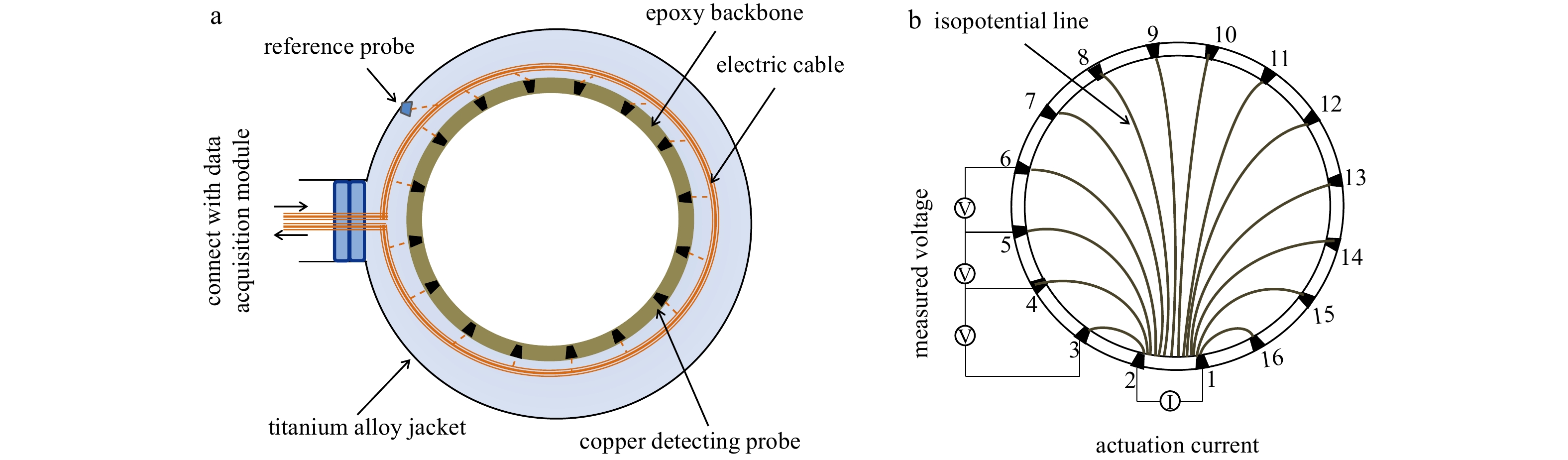
An epoxy tube fitted with connecting electrical cable serves as the insulating backbone of the electrical probes. Totally 16 copper electrodes are embedded in the epoxy tube at the same height (120 mm from the bottom of the vessel, “a-a” in Fig. 1b). Hereafter, the “a-a” plane is called the ERT monitoring plane. The epoxy tube is enclosed and sealed into a titanium alloy jacket to form a high-pressure vessel (Fig. 2a). The width and length of each electrode are 5 mm and 20 mm, respectively, and the distance between the electrodes is 5 mm (Li et al., 2020d). A ground electrode is installed to provide a ground reference to the sixteen measuring electrodes. These electrodes are connected to the data acquisition module (ITS P2000; Industrial Tomography Systems Ltd, UK), which is controlled by software provided by the manufacturer. The temperature and pressure are acquired by a self-developed code.
Figure
2.
Top-view diagram of the high-pressure chamber containing ITS spool (a), and four-electrode probe adjacent measurement strategy (b). In b, the No. 1 and No. 2 electrodes act as source electrodes, while the other 14 probes act as receiver electrodes.
In this experiment, medium–coarse sand from Qingdao beach was used as host sediment. Grain size of the beach sand ranges from 0.05 mm to 0.85 mm, with a medium grain size of 0.31 mm. A detailed discussion about the particle size distribution characteristics, as well as the determination of total porosity and permeability, could be found in our previous work (Dong et al., 2020; Li et al., 2018). Sodium chloride solution with a salinity of 3.5 wt.% was used to simulate the pore water. The purity of the methane gas is 99.99%.
2.2
ERT data acquisition and processing method
To visually observe and monitor the real-time reaction processes inside the high-pressure vessel, different multi-electrode driving patterns have been documented by previous studies (Cui et al., 2016). In this work, a four-electrode initiating and measuring method is involved and connected with the ITS P2000.
The actuation current, which remains constant throughout the process, is injected and exported from each of two of the neighboring electrodes by turns, and then the dynamic voltages between each two of the other fourteen neighboring electrodes are obtained and transformed into conductivities (Fig. 2b). Therefore, 104 conductivity (the inverse of electrical resistivity) values are obtained within one measuring circle. The average of the 104 conductivities reflects the overall transient state of the ERT monitoring plane, which is defined as the average plane conductivity in this manuscript.
A variety of algorithms were reported in reconstructing the dynamic electrical conductivity field. The non-linear method was supposed to be more accurate and tends to reduce artifacts (Asgarifar et al., 2010; Kotzé et al., 2019). However, it will consume many computational resources and therefore may not be suitable for high-speed and real-time industrial applications.
The linear back projection (LBP) methodology is considered to be the most robust methodology due to its fast-computational speed and algorithm simplicity (Bolton et al., 2007; Smyl, 2020). The LBP method is used in our study to reconstruct the dynamic real-time electrical conductivity field during hydrate formation.
The average hydrate saturation in the sediment is determined independently from pore pressure and temperature.
where P1 (MPa) represents the pressure in the vessel at initial state; T1 (K) represents the temperature at initial state; P2 and T2 represent the real-time pressure-temperature conditions in the vessel; Mh is the molar mass of natural gas hydrate, Mh=122.02 g/mol; R is universal gas constant, R=8.314 J/(mol·K); ρh is the density of the methane hydrate, ρh =0.91 g/cm3; Vp is the pore volume of the sediment pressed into the vessel, Vp= 249.56 mL; whereas the Vg is the real-time gas volume contained in the system, Vg =153.5 mL.
It should be noted that the volume occupied by fluid in the sediment decreases with the increase in hydrate saturation, leading to a decrease in Vg. However, the pore volume in this experiment is much smaller than the volume of gas supply pipe. Therefore, the influence of Vp on Vg is neglected in this paper.
The Archie equation is an empirical relation to calculate hydrate saturation from electrical resistivity. The electrical resistivity index is introduced to describe the increase in electrical resistivity caused by hydrate formation within the sediment. Hence the Archie equation for hydrate saturation prediction could be written as Eq. (2).
where F is the formation factor; $ I $ represents the electrical resistivity index; Rw, R0, and Rt are electrical resistivity of the connate water, hydrate-free water-saturated sediments, and hydrate-bearing sediment in Ω·m, respectively; σw, σ0, and σt are electrical conductivity of the connate water, hydrate-free water-saturated sediments, and hydrate-bearing sediment in S/m, respectively; φ is the total porosity of the sediment, φ=41%; a and m are Archie constant; Sh is the hydrate saturation; n is the saturation exponent, which is mainly determined by hydrate saturation itself providing the host sediment is definite (Cook and Waite, 2018).
In field geophysical application, $ \varphi $ is normally derived from bulk density logging, whereas a and m are derived based on the cross plot between the porosity and formation factor. There are great discrepancies among hydrate saturation prediction results from different literatures because of the value of a and m. However, in this experiment, the formation factor and the resistivity of hydrate-bearing sediment could be obtained directly from the experiment. The hydrate saturation could be derived from Eq. (3).
where $\bar{{\sigma }_\mathrm{t}}$ represents the average plane conductivity obtained from ERT module. The average hydrate saturation ${\bar{S}}_\mathrm{h}$ could be derived from Eq. (1). Therefore, we obtain an equation for saturation exponent by the combination of Eqs (4) and (1).
Finally, we could predict hydrate distribution within the sediment from the real-time electrical conductivity distribution field through Eq. (3). It is worthy noting that the above equations are based on the assumptions that no free gas exist in the system. Once we inject free gas directly into the vessel, the ERT results might underestimate the absolute hydrate saturation due to existence of free gas. However, this would have little influence for relative accumulation state in an enclosed system.
2.3
Experimental procedures
To clarify the comparability of this study to field conditions, we firstly tested the conductivity change behaviors of both brine and brine-saturated sediment with temperature using the 2D ERT hydrate monitoring device. This process also helps to determine the formation factor, which was defined as the ratio of the resistivity of fully brine-saturated sediment (R0) to the resistivity of the connate water (Rw) in Eq. (2).
Firstly, the vessel was filled with the brine at room temperature (20°C). Then we started the temperature control module to cool the vessel at a rate of 1°C/min and initiated the ERT monitoring process simultaneously. The average plane conductivity was recorded during cooling. The beach sand was washed carefully with distilled water and dried. Then the sand was poured into the brine gradually to avoid the formation of gas bubbles in the sediment. Then constant axial stress of 0.5 MPa was applied to the sample for 2 h. Excessive water located above the saturated-sediment was pumped out. This process ensures that the sediment was saturated homogeneously. Finally, the vessel was warmed-up at a rate of 1°C/min and the ERT values were acquired simultaneously.
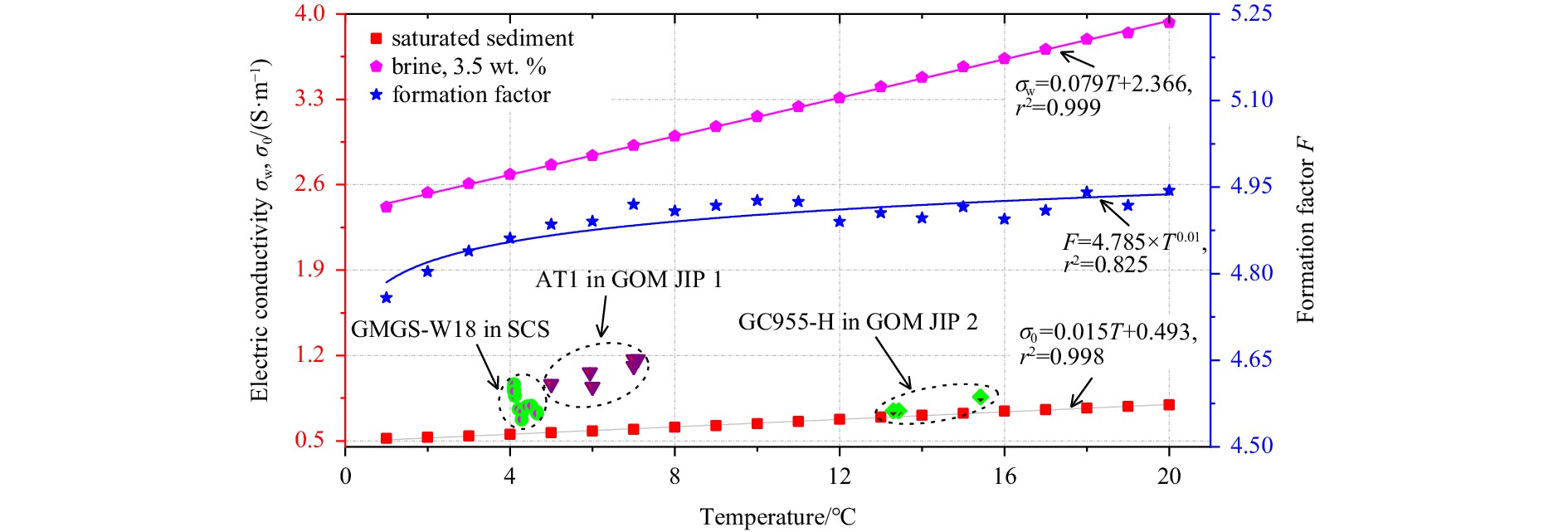
The relationships between temperature and conductivity of pore-water and saturated sediment could be obtained from the above procedures. Figure 3 shows a comparison of pore water, brine-saturated sediment, and typical marine field conditions. The correlation data are from the GMGS-W18 in the Shenhu area, northern South China Sea (Li et al., 2019a; Li et al., 2019b; Li et al., 2020b; Li et al., 2020e; Zhang et al., 2019; Zhao et al., 2020) and the AT1 and GC955-H, Gulf of Mexico, USA (Merey, 2019). It is obvious that the laboratory brine-saturated sediment system is very close to the marine sediment. Therefore, the experiment in this manuscript is comparable to field conditions.
Figure
3.
Conductivity clarifications for pore water (sodium chloride solution with a salinity of 3.5 wt.%) and brine-saturated sediment. The temperature for AT1 and GC955-H in the Gulf of Mexico, USA are obtained from the drilling operation. The temperature for GMGS-W18 is predicted according to the seafloor temperature (3.76°C) and geothermal gradient (63°C/km) (Liao et al., 2016; Zhang et al., 2019). JIP: Joint Industrial Program.
Figure 3 also depicts the relationship between temperature and formation factor. It is clear to see that both the electrical conductivity of the brine and brine-saturated sediment decrease linearly with the decrease in temperature. The formation factor of the sediment fluctuates between 4.76 and 4.94, with an average value of 4.85. The best-fit empirical function for the conductivity of the pore-water, the conductivity of the brine-saturated sediment, and the formation factor are shown in Eqs (6)–(8), respectively.
The hydrate distribution field on the ERT monitoring plane could be obtained by combining Eqs (3)–(8).
The hydrate forming processes were carried out following the procedures described below. Two parallel experiments were conducted in this study. The duplicated test showed good agreement with the tested one. One of the experiments is discussed.
The vessel is fully filled with brine-saturated sediment and placed into the cold-chamber (1°C). The temperature of the sediment was maintained at 1°C for more than 5 h before gas injection. Conductivity distribution at 1°C was taken as reference (Fig. 4a). Figure 4a indicates that conductivity at the ERT monitoring plane is evenly distributed before gas injection. The average plane conductivity is 5.22 mS/cm at 1°C, which is consistent with that observed in Fig. 4. Then methane was injected into the vessel from the gas injection inlet. The gas injection rate was controlled at 10 standard cubic centimeters per minute (SCCM) by a mass flow controller. The targeted pore pressure of the experiment is controlled around 80×105 Pa.
Figure
4.
Gas injection-induced concentric-zonal conductivity distribution at 1°C. a. Uniform distribution before gas injection; b. heterogeneous distribution after gas injection.
We observed that gas injection process broke-up the uniformly distributed conductivity field. Conductivity at the center of the ERT monitoring plane decreased greatly while the peripheral part remains unchanged. As a result, concentric-zonal conductivity distribution characteristics were observed and expanded gradually from the center to the periphery, which is shown in Fig. 4b.
Concentric-zonal conductivity distribution implies a concentric-zonal distribution of gas and water within the sediment. Gas diffusion is markedly strong at the center while weak at the peripheral part. Figure 4b could be viewed as the initial conductivity distribution state for the hydrate-forming simulation. The temperature of the sediment now remained at 1°C. The pressure in the vessel would drop due to the formation of hydrate. When the pressure in the vessel remains unchanged for more than 5 h, the vessel was reloaded with methane to about 80×105 Pa.
3.
Results and discussion
3.1
Average conductivity and saturation exponent
During the entire hydrate formation process, the temperature in the sediment was kept stable at 1°C (±0.5°C). The pore pressure of the sediment, the average conductivity at the ERT monitoring plane, and the average hydrate saturation from Eq. (1) are shown in Fig. 5. The pore pressure decreases with the formation of the hydrate. When the pressure decreased to a certain value and kept constant for more than 5 h, gas was injected at a rate of less than 10 SCCM until the pore pressure reached 80×105 Pa. Three gas injection cycles were applied in this experiment (t1, t2, and t3 in Fig. 5).
Figure
5.
Measured pore pressure (black solid line) (Li et al., 2020d), average conductivity (blue solid line), and average hydrate saturation from Eq. (1) (red solid line) versus experimental time. Δσ1 is the decrease in the average conductivity caused by the second gas injection or loading; Δσ2 is the decrease in the average conductivity caused by the third gas injection.
It could be seen from Fig. 5 that the pore pressure rises continuously to 80×105 Pa within each pressure loading cycle. However, each gas injection operation causes a plummet in the average conductivity (Δσ1 and Δσ2 in Fig. 5). In the early stages of the experiment (≤155 h) when hydrate saturation is less than 11%, we could see little change in the average conductivity. After that, the average conductivity decreases nonlinearly with the formation of the hydrate. The average conductivity fluctuates within certain scopes at some special time-intervals. Furthermore, the magnitude of the average conductivity fluctuation becomes larger with the increase in average hydrate saturation.
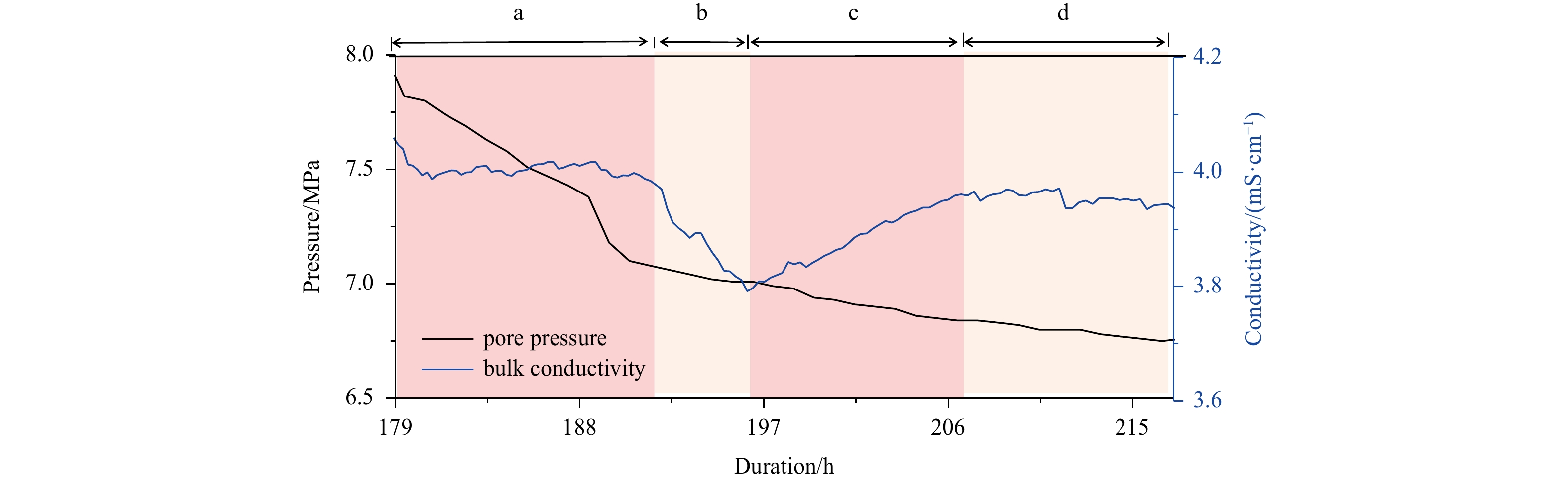
To further investigate the fluctuation behaviors in the average conductivity, we made a comparison between the pore pressure and average conductivity at the early stage of t2 (time interval of 179–217 h) in Fig. 6. According to the changes in the average conductivity, the experimental duration from 179 h to 217 h is divided into four sub-intervals, noted as a–d in Fig. 6. The pore pressure declines rapidly during sub-interval a, and then decreases gradually and smoothly during sub-intervals b–d. Nevertheless, the average conductivity showed four-stages behavior, which is characterized by constant (a) → decline (b) → rebound (c) →constant (d).
Figure
6.
Evolution of pore pressure and average conductivity from 179 h to 217 h.
Hydrate formation itself tends to reduce the conductivity, while salt-removing tends to enhance the conductivity of the sediment. Therefore, the average conductivity of the hydrate-bearing sediment is determined by the combination of hydrate formation and associated salt-removing effect. Providing that hydrate formation induced conductivity decline rate is ${d}{\rho }_\mathrm{h}$, while the salt-removing induced conductivity rise rate is ${d}{\rho }_\mathrm{s}$. The difference between the ${d}{\rho }_\mathrm{h}$ and ${d}{\rho }_\mathrm{s}$ determines the change in average conductivity. The fluctuation of the average conductivity disappears when ${d}{\rho }_\mathrm{h}\approx {d}{\rho }_\mathrm{s}$. When the hydrate formation process becomes dominant (with a high synthesizing rate), the average plane conductivity tends to decline, and vice versa.
As mentioned above, the fluctuation magnitude of the average conductivity becomes stronger with the increase in average hydrate saturation, which could be attributed to the re-distribution of salt concentration. Motivated by the local salinity differences, salt ions would disperse and migrate once the salt-removing effect happens. Thereby low hydrate saturation indicates enough pore space for ions transformation, which may also enhance the moderating effect of pore water on ions concentration. However, with the increase in hydrate saturation, part of the salt ion transformation pathways might be blocked by hydrate (Chen et al., 2018). The moderating effect of pore water on ions concentration becomes weaker. Consequently, there is a severe fluctuation in average conductivity.
We evaluated the hydrate saturation exponent based on the average hydrate saturation and average conductivity showed in Fig. 6. The result is shown in Fig. 7, the saturation exponent ranges between 0.25 and 4.85, with an average of 0.92 and a mathematical median value of 2.30. The saturation exponent decreases rapidly below 7% hydrate saturation. When average hydrate saturation exceeds 16%, the predicted saturation exponent remains stable at 1±0.2, which is much lower than the value n=2) suggested by Pearson et al. (1983). The result in Fig. 7 would be coupled with Eq. (4) to estimate spatial and temporal distributions of hydrate.
Figure
7.
Relationship between average hydrate saturation and saturation exponent in this experiment.
Although the average conductivity fluctuates because of the influence of the salt-removing effect, the final conductivity value is determined by the amount of hydrate in the sediment. Therefore, the deviation of real-time ERT monitoring results to the initial state (shown in Fig. 4b) could be used as an indicator for hydrate saturation distribution. To identify local preferential hydrate-forming positions and their alteration with time, real-time ERT data were acquired and imaged via ITS P2000. Some of the real-time conductivity fields at the ERT monitoring plane are imaged in Fig. 8.
Figure
8.
Conductivity fields at typical time nodes. The conductivity distribution after gas injection (Fig. 5b) was taken as reference.
The conductivity fields evolve heterogeneously throughout the experiment. In Fig. 8, the conductivity distribution seems to be scattered within the first few hours (Fig. 8, t=6 h). We attribute this to the randomness of hydrate nucleation. The magnitude of the conductivity field decreases with time. Finally, a concentric-zonal structure of conductivity field forms (Fig. 8, t=310 h). The conductivity intensity within the same concentric-zonal area becomes evenly distributed.
The discrete plane conductivity distribution could be expressed via a continuous survey line in each sectional conductivity field. Herein, the 45° line in the 2D conductivity field was taken as the survey line (see Fig. 8, t=6 h). The ERT measuring results on the survey line were taken at two minutes interval and then stacked based on time series. The dynamic evolutionary behavior of the conductivity along the 45° line is shown in Fig. 9.
Figure
9.
Dynamic evolutionary behavior of conductivity value along the 45° line of the monitoring section in Fig. 8. The gas injection tunnel locates at the middle of the vessel, where Y=0.0 cm.
The middle of the Y-axis in Fig. 9 represents the original gas injection tunnel. Concentric-zonal conductivity distribution characteristics could be observed throughout the experiment. At the early stage of the experiment, the lateral diffusion of methane gas controlled the concentric-zonal conductivity distribution. The conductivity rises laterally with the increase of the distance to the center. At the late stages of the experiment, the concentric-zonal conductivity distribution is mainly controlled by the distribution of hydrate. The “phase inverse” in the concentric-zonal conductivity distribution was observed during the middle stage of the experiment (170–200 h). The minimum conductivity zonal area distributed at a specific radius ranges to the center part since phase inverse.
Heterogeneous conductivity distribution could be observed during sub-interval a1 and a2 in Fig. 9. The local conductivity around the center decreased with time, followed by a slight inclination before becoming stable. This is consistent with the fluctuation of average conductivity (Fig. 6). Therefore, the combination of hydrate formation and salt-removing effect is confirmed to be the main controlling factor for fluctuation of the conductivities at the ERT monitoring plane.
The heterogeneous conductivity decreasing process indicates heterogeneous hydrate synthesizing process. We calculate hydrate spatial and temporal distribution at the ERT monitoring plane by a combination of Eqs (4)–(8). Since the temperature is controlled at 1°C, the conductivity of the brine and the brine-saturated sediment are 2.415 S/m and 0.518 S/m, respectively. The formation factor is 4.76. Hydrate saturation distributions at the ERT monitoring plane are shown in Fig. 10.
Figure
10.
Hydrate distribution behaviors at typical time nodes at the electrical resistivity tomography monitoring plane.
Figure 10 shows real-time preferential hydrate-forming positions. Alteration in preferential hydrate-forming positions tends to improve the homogeneity within the same concentric zonal area, while enhances anisotropy among different concentric zonal areas. At the end of the experiment (t=310 h in Fig. 10), we could see an obvious radial saturation gradient at the ERT monitoring plane. The maximum hydrate saturation within the sediment is 49.5%, with an average hydrate saturation of 38.5%. The alteration in local preferential hydrate-forming positions could also be attributed to the combination of hydrate formation and salt-removing effect.
This study demonstrates the utility of the ERT method for hydrate mapping in lab-scale. The results indicate that the average electrical conductivity decreases nonlinearly with the formation of the hydrate. At some special time-intervals, the average conductivity fluctuates within a certain scope. The plane conductivity fields evolve heterogeneously and the local preferential hydrate-forming positions alternate throughout the experiment.
Current study implies the utility of the ERT method for hydrate mapping in lab-scale. We attempted to match hydrological regimes and geological conditions of those of a real submarine environment. However, some factors involved in real submarine sediments were not taken into consideration due to experimental scale limitations. To meet the need of complicated simulation conditions requires an upgrade of the experimental scale or the installation of special structures into the vessel.
4.
Conclusions
This study developed a remote hydrate detecting experimental device based on ERT technology. Methane gas was injected from the center of the bottom flange with several cycles to simulate hydrate formation process at gas-water-sediment multi-phase scenarios. Hydrate formation was conducted at 1°C. Both the average conductivity and the conductivity field were comprehensively studied. The Archie equation is introduced to derive spatial and temporal distributions of hydrate within the sediment. The experiment yielded the following results.
(1) Generally, the average electrical conductivity decreased nonlinearly with the increase of average hydrate saturation. However, we still observed certain fluctuations of the average conductivity at some special time-intervals, namely, the average electrical conductivity increased slightly with the gas consumption (i.e. hydrate formation). This phenomenon was unlikely to occur if the average electrical conductivity is dominated solely by hydrate formation. As a result, we speculate that the hydrate formation process was accompanied by a certain remarkable mass-transfer, either three-dimensional or two-dimensional. And the salt-removal effect was responsible for such a remarkable mass-transfer.
(2) The conductivity field changed non-homogeneously throughout the experimental duration, indicating that the preferential hydrate-forming positions alternated throughout the experiment. Under the condition that gas was injected at the center of bottom flange, the hydrate distribution at the ERT monitoring plane showed obvious concentric-zonal characteristics with a radial saturation gradient. This was quite important since it inspired us the importance of water activity (seepage dominated by salinity difference) in hydrate accumulation processes in nature.
(3) The current study indicates anisotropic and heterogeneous hydrate formation processes under the condition of gas-water two-phase conditions. We speculate that salt-removal effect and hydrate formation itself are the main determinants of spatial and temporal hydrate distribution characteristics. Owing to the limitation of the experimental scale, the current experiment doesn’t take the influences of geochemical and geophysical characteristics into consideration, although they might play crucial roles in hydrate accumulation mechanisms in nature. Updating the experimental scale or installing some special structures into the vessel are needed to simulate more complicated situations.
Asgarifar S, Frounchi J, Zarifi M H, et al. 2010. A novel two-stage genetic algorithm for image reconstruction of electrical resistance tomography. International Journal of Modeling, Simulation, and Scientific Computing, 1(4): 523–542
[2]
Attias E, Amalokwu K, Watts M, et al. 2020. Gas hydrate quantification at a pockmark offshore Norway from joint effective medium modelling of resistivity and seismic velocity. Marine and Petroleum Geology, 113: 104151. doi: 10.1016/j.marpetgeo.2019.104151
[3]
Bolton G T, Bennett M, Wang Mi, et al. 2007. Development of an electrical tomographic system for operation in a remote, acidic and radioactive environment. Chemical Engineering Journal, 130(2−3): 165–169. doi: 10.1016/j.cej.2006.06.019
[4]
Chaouachi M, Falenty A, Sell K, et al. 2015. Microstructural evolution of gas hydrates in sedimentary matrices observed with synchrotron X-ray computed tomographic microscopy. Geochemistry, Geophysics, Geosystems, 16(6): 1711–1722
[5]
Chen Qiang, Diao Shaobo, Ye Yuguang. 2013. Detecting hydrate in porous media using electrical resistance. In: Ye Yuguang, Liu Changling, eds. Natural Gas Hydrates: Experimental Techniques and Their Applications. Berlin, Heidelberg: Springer, 127–140
[6]
Chen Qiang, Liu Changling, Xing Lanchang, et al. 2016. Resistivity variation during hydrate formation in vertical inhomogeneous distribution system of pore water. Acta Petrolei Sinica, 37(2): 222–229
[7]
Chen Yufeng, Wu Nengyou, Liang Deqing, et al. 2018. Numerical simulation on the resistivity of hydrate-bearing sediment based on fractal pore model. Natural Gas Industry, 38(11): 128–134
[8]
Chong Zhengrong, Yang She Hern Bryan, Babu P, et al. 2016. Review of natural gas hydrates as an energy resource: prospects and challenges. Applied Energy, 162: 1633–1652. doi: 10.1016/j.apenergy.2014.12.061
[9]
Cook A E, Waite W F. 2018. Archie’s saturation exponent for natural gas hydrate in coarse-grained reservoirs. Journal of Geophysical Research: Solid Earth, 123(3): 2069–2089. doi: 10.1002/2017JB015138
[10]
Cui Yudong, Lu Cheng, Wu Mingtao, et al. 2018. Review of exploration and production technology of natural gas hydrate. Advances in Geo-Energy Research, 2(1): 53–62. doi: 10.26804/ager.2018.01.05
[11]
Cui Ziqiang, Wang Qi, Xue Qian, et al. 2016. A review on image reconstruction algorithms for electrical capacitance/resistance tomography. Sensor Review, 36(4): 429–445. doi: 10.1108/SR-01-2016-0027
[12]
Dong Lin, Li Yanlong, Liao Hualin, et al. 2020. Strength estimation for hydrate-bearing sediments based on triaxial shearing tests. Journal of Petroleum Science and Engineering, 184: 106478. doi: 10.1016/j.petrol.2019.106478
[13]
Dong Huaimin, Sun Jianmeng, Zhu Jinjiang, et al. 2019. Developing a new hydrate saturation calculation model for hydrate-bearing sediments. Fuel, 248: 27–37. doi: 10.1016/j.fuel.2019.03.038
[14]
Du Frane W L, Stern L A, Constable S, et al. 2015. Electrical properties of methane hydrate + sediment mixtures. Journal of Geophysical Research: Solid Earth, 120(7): 4773–4783. doi: 10.1002/2015JB011940
[15]
Du Frane W L, Stern L A, Weitemeyer K A, et al. 2011. Electrical properties of polycrystalline methane hydrate. Geophysical Research Letters, 38(9): L09313
[16]
Fu Chao, Li Shengli, Yu Xinghe, et al. 2019. Patterns of gas hydrate accumulation in mass transport deposits related to canyon activity: example from Shenhu drilling area in the South China Sea. Acta Oceanologica Sinica, 38(5): 118–128. doi: 10.1007/s13131-019-1443-1
Heeschen K, Spangenberg E, Schicks J M, et al. 2014. Simulating the gas hydrate production test at Mallik using the pilot scale pressure reservoir LARS. In: EGU General Assembly Conference Abstracts. Vienna: EGU
[19]
Jana S, Ojha M, Sain K, et al. 2017. An approach to estimate gas hydrate saturation from 3-D heterogeneous resistivity model: a study from Krishna-Godavari basin, Eastern Indian offshore. Marine and Petroleum Geology, 79: 99–107. doi: 10.1016/j.marpetgeo.2016.11.006
[20]
Koh C A, Sum A K, Sloan E D. 2012. State of the art: natural gas hydrates as a natural resource. Journal of Natural Gas Science and Engineering, 8: 132–138. doi: 10.1016/j.jngse.2012.01.005
[21]
Konno Y, Kato A, Yoneda J, et al. 2019. Numerical analysis of gas production potential from a gas-hydrate reservoir at Site NGHP-02-16, the Krishna–Godavari Basin, offshore India–Feasibility of depressurization method for ultra-deepwater environment. Marine and Petroleum Geology, 108: 731–740. doi: 10.1016/j.marpetgeo.2018.08.001
[22]
Kotzé R, Adler A, Sutherland A, et al. 2019. Evaluation of Electrical Resistance Tomography imaging algorithms to monitor settling slurry pipe flow. Flow Measurement and Instrumentation, 68: 101572. doi: 10.1016/j.flowmeasinst.2019.101572
[23]
Li Yanlong, Chen Qiang, Wu Nengyou, et al. 2020a. Core-scale application of electrical resistivity tomography technology on visual detection of natural gas hydrate. Geological Review, 66(S1): 84–86
[24]
Li Yanlong, Hu Gaowei, Wu Nengyou, et al. 2019a. Undrained shear strength evaluation for hydrate-bearing sediment overlying strata in the Shenhu area, northern South China Sea. Acta Oceanologica Sinica, 38(3): 114–123. doi: 10.1007/s13131-019-1404-8
[25]
Li Chengfeng, Liu Changling, Hu Gaowei, et al. 2019b. Investigation on the multiparameter of hydrate-bearing sands using nano-focus X-ray computed tomography. Journal of Geophysical Research:Solid Earth, 124(3): 2286–2296. doi: 10.1029/2018JB015849
[26]
Li Yanlong, Liu Lele, Jin Yurong, et al. 2021. Characterization and development of natural gas hydrate in marine clayey-silt reservoirs: a review and discussion. Advances in Geo-Energy Research, 5(1): 75–86. doi: 10.46690/ager.2021.01.08
[27]
Li Yanlong, Liu Changling, Liu Lele, et al. 2018. Experimental study on evolution behaviors of triaxial-shearing parameters for hydrate-bearing intermediate fine sediment. Advances in Geo-Energy Research, 2(1): 43–52. doi: 10.26804/ager.2018.01.04
[28]
Li Yanlong, Ning Fulong, Wu Nengyou, et al. 2020b. Protocol for sand control screen design of production wells for clayey silt hydrate reservoirs: a case study. Energy Science & Engineering, 8(5): 1438–1449
[29]
Li Yanlong, Sun Hailiang, Liu Changling, et al. 2020c. Application of ERT to hydrate monitoring: take ice as substitute. Marine Geology Frontiers, 36(3): 65–71
[30]
Li Yanlong, Sun Hailiang, Meng Qingguo, et al. 2019c. 2-D electrical resistivity tomography assessment of hydrate formation in sandy sediments. Natural Gas Industry, 39(10): 132–138
[31]
Li Yanlong, Sun Hailiang, Meng Qingguo, et al. 2020d. 2-D electrical resistivity tomography assessment of hydrate formation in sandy sediments. Natural Gas Industry B, 7(3): 278–284. doi: 10.1016/j.ngib.2019.10.010
[32]
Li Yanlong, Wu Nengyou, Ning Fulong, et al. 2020e. Hydrate-induced clogging of sand-control screen and its implication on hydrate production operation. Energy, 206: 118030. doi: 10.1016/j.energy.2020.118030
[33]
Liao Jing, Gong Jianming, Lü Wanjun, et al. 2016. Simulation of the accumulation process of biogenic gas hydrates in the Shenhu area of northern South China Sea. Acta Geologica Sinica (English Edition), 90(6): 2285–2286. doi: 10.1111/1755-6724.13048
[34]
Lim D, Ro H, Seo Y J, et al. 2017. Electrical resistivity measurements of methane hydrate during N2/CO2 gas exchange. Energy & Fuels, 31(1): 708–713
[35]
Liu Changling, Li Yanlong, Liu Lele, et al. 2020a. An integrated experimental system for gas hydrate drilling and production and a preliminary experiment of the depressurization method. Natural Gas Industry B, 7(1): 56–63. doi: 10.1016/j.ngib.2019.06.003
[36]
Liu Changling, Li Yanlong, Sun Jianye, et al. 2017. Gas hydrate production test: from experimental simulation to field practice. Marine Geology & Quaternary Geology, 37(5): 12–26
[37]
Liu Tao, Liu Xuewei, Zhu Tieyuan. 2020b. Joint analysis of P-wave velocity and resistivity for morphology identification and quantification of gas hydrate. Marine and Petroleum Geology, 112: 104036. doi: 10.1016/j.marpetgeo.2019.104036
[38]
Liu Yang, Xian Chenggang, Li Zhe, et al. 2020c. A new classification system of lithic-rich tight sandstone and its application to diagnosis high-quality reservoirs. Advances in Geo-Energy Research, 4(3): 286–295. doi: 10.46690/ager.2020.03.06
[39]
Lu R, Stern L A, Du Frane W L, et al. 2019. The effect of brine on the electrical properties of methane hydrate. Journal of Geophysical Research: Solid Earth, 124(11): 10877–10892. doi: 10.1029/2019JB018364
[40]
Malinverno A, Kastner M, Torres M E, et al. 2008. Gas hydrate occurrence from pore water chlorinity and downhole logs in a transect across the northern Cascadia margin (Integrated Ocean Drilling Program Expedition 311). Journal of Geophysical Research: Solid Earth, 113(B8): B08103
[41]
McConnell D R, Zhang Zijian, Boswell R. 2012. Review of progress in evaluating gas hydrate drilling hazards. Marine and Petroleum Geology, 34(1): 209–223. doi: 10.1016/j.marpetgeo.2012.02.010
[42]
Merey Ş. 2019. Evaluation of drilling parameters in gas hydrate exploration wells. Journal of Petroleum Science and Engineering, 172: 855–877. doi: 10.1016/j.petrol.2018.08.079
[43]
Pan Haojie, Li Hongbing, Chen Jingyi, et al. 2020. Quantification of gas hydrate saturation and morphology based on a generalized effective medium model. Marine and Petroleum Geology, 113: 104166. doi: 10.1016/j.marpetgeo.2019.104166
[44]
Pandey L, Sain K, Joshi A K. 2019. Estimate of gas hydrate saturations in the Krishna-Godavari basin, eastern continental margin of India, results of expedition NGHP-02. Marine and Petroleum Geology, 108: 581–594. doi: 10.1016/j.marpetgeo.2018.12.009
[45]
Pearson C F, Halleck P M, McGuire P L, et al. 1983. Natural gas hydrate deposits: a review of in situ properties. The Journal of Physical Chemistry, 87(21): 4180–4185. doi: 10.1021/j100244a041
[46]
Permyakov M E, Manchenko N A, Duchkov A D, et al. 2017. Laboratory modeling and measurement of the electrical resistivity of hydrate-bearing sand samples. Russian Geology and Geophysics, 58(5): 642–649. doi: 10.1016/j.rgg.2017.04.005
[47]
Priegnitz M, Thaler J, Spangenberg E, et al. 2013. A cylindrical electrical resistivity tomography array for three-dimensional monitoring of hydrate formation and dissociation. Review of Scientific Instruments, 84(10): 104502. doi: 10.1063/1.4825372
[48]
Priegnitz M, Thaler J, Spangenberg E, et al. 2014. Spatial resolution of gas hydrate and permeability changes from ERT data in LARS simulating the Mallik gas hydrate production test. In: EGU General Assembly Conference. Vienna: EGU
[49]
Priegnitz M, Thaler J, Spangenberg E, et al. 2015. Characterizing electrical properties and permeability changes of hydrate bearing sediments using ERT data. Geophysical Journal International, 202(3): 1599–1612. doi: 10.1093/gji/ggv245
[50]
Sahoo S K, Marín-Moreno H, North L J, et al. 2018. Presence and consequences of coexisting methane gas with hydrate under two phase water-hydrate stability conditions. Journal of Geophysical Research: Solid Earth, 123(5): 3377–3390. doi: 10.1029/2018JB015598
[51]
Santamarina J C, Ruppel C. 2008. The impact of hydrate saturation on the mechanical, electrical, and thermal properties of hydrate-bearing sand, silts, and clay. In: Proceedings of the 6th International Conference on Gas Hydrates. Vancouver, Canada: Society of Exploration Geophysicists
[52]
Shankar U, Riedel M. 2014. Assessment of gas hydrate saturation in marine sediments from resistivity and compressional-wave velocity log measurements in the Mahanadi Basin, India. Marine and Petroleum Geology, 58: 265–277. doi: 10.1016/j.marpetgeo.2013.10.007
[53]
Smyl D. 2020. Electrical tomography for characterizing transport properties in cement-based materials: a review. Construction and Building Materials, 244: 118299. doi: 10.1016/j.conbuildmat.2020.118299
[54]
Spangenberg E. 2001. Modeling of the influence of gas hydrate content on the electrical properties of porous sediments. Journal of Geophysical Research: Solid Earth, 106(B4): 6535–6548. doi: 10.1029/2000JB900434
[55]
Spangenberg E, Kulenkampff J. 2006. Influence of methane hydrate content on electrical sediment properties. Geophysical Research Letters, 33(24): L24315. doi: 10.1029/2006GL028188
[56]
Spangenberg E, Kulenkampff J, Naumann R, et al. 2005. Pore space hydrate formation in a glass bead sample from methane dissolved in water. Geophysical Research Letters, 32(24): L24301. doi: 10.1029/2005GL024107
[57]
Sun Jianye, Li Chengfeng, Hao Xiluo, et al. 2020. Study of the surface morphology of gas hydrate. Journal of Ocean University of China, 19(2): 331–338. doi: 10.1007/s11802-020-4039-7
[58]
Sun Hailiang, Li Yanlong, Liu Changling, et al. 2019. Electrical resistance tomography and the application in the simulation experiment of hydrate mining. Acta Metrologica Sinica, 40(3): 455–461
[59]
Waite W F, Santamarina J C, Cortes D D, et al. 2009. Physical properties of hydrate-bearing sediments. Reviews of Geophysics, 47(4): RG4003
[60]
Walsh M. 2014. Laboratory and high-pressure flow loop investigation of gas hydrate formation and distribution using electrical tomography. In: Proceedings of the 8th International Conference on Gas Hydrates (ICGH8–2014). Beijing: China Geological Survey
[61]
Wang Xiujuan, Wu Shiguo, Lee Myung, et al. 2011. Gas hydrate saturation from acoustic impedance and resistivity logs in the Shenhu area, South China Sea. Marine and Petroleum Geology, 28(9): 1625–1633. doi: 10.1016/j.marpetgeo.2011.07.002
[62]
Wu Nengyou, Li Yanlong, Wan Yizhao, et al. 2021. Prospect of marine natural gas hydrate stimulation theory and technology system. Natural Gas Industry B, 8(2): 173–187. doi: 10.1016/j.ngib.2020.08.003
[63]
Wu Nengyou, Liu Changling, Hao Xiluo. 2018. Experimental simulations and methods for natural gas hydrate analysis in China. China Geology, 1(1): 61–71. doi: 10.31035/cg2018008
[64]
Yang Lei, Falenty A, Chaouachi M, et al. 2016. Synchrotron X-ray computed microtomography study on gas hydrate decomposition in a sedimentary matrix. Geochemistry, Geophysics, Geosystems, 17(9): 3717–3732
[65]
Ye Jianliang, Qin Xuwen, Xie Wenwei, et al. 2020. The second natural gas hydrate production test in the South China Sea. China Geology, 3(2): 197–209
[66]
Zhang Wei, Liang Jinqiang, Wei Jiangong, et al. 2019. Origin of natural gases and associated gas hydrates in the Shenhu area, northern South China Sea: results from the China gas hydrate drilling expeditions. Journal of Asian Earth Sciences, 183: 103953. doi: 10.1016/j.jseaes.2019.103953
[67]
Zhao Jiafei, Liu Yulong, Guo Xianwei, et al. 2020. Gas production behavior from hydrate-bearing fine natural sediments through optimized step-wise depressurization. Applied Energy, 260: 114275. doi: 10.1016/j.apenergy.2019.114275
Hui Pan, Hui Xie, Zhongxian Zhao, et al. Quaternary gas hydrate dissociation promotes the formation of Shenhu Canyon Group in the South China Sea. Frontiers in Marine Science, 2025, 12 doi:10.3389/fmars.2025.1530207
2.
Jilun Weng, Tao He. Research on resistivity characteristics of grain-coating and pore-filling hydrates in different sediment packings based on voxelated 3D models. Gas Science and Engineering, 2025, 133: 205501. doi:10.1016/j.jgsce.2024.205501
3.
Kaan Koca, Eckhard Schleicher, André Bieberle, et al. GravelSens: A Smart Gravel Sensor for High-Resolution, Non-Destructive Monitoring of Clogging Dynamics. Sensors, 2025, 25(2): 536. doi:10.3390/s25020536
4.
Chenyi Zhang, Tingting Luo, Yong Xue, et al. Geophysical Properties of Hydrate-Bearing Silty-Clayey Sediments with Different Compaction Patterns. Energy & Fuels, 2024, 38(21): 20607. doi:10.1021/acs.energyfuels.4c04116
5.
Qiaobo Hu, Yanlong Li, Nengyou Wu, et al. Influences of stress state on compressional wave velocity of sandy hydrate-bearing sediment: Experiments and modeling. Geoenergy Science and Engineering, 2024, 234: 212683. doi:10.1016/j.geoen.2024.212683
6.
Yang Meng, Bingyue Han, Jiguang Wang, et al. Hydrate Blockage in Subsea Oil/Gas Pipelines: Characterization, Detection, and Engineering Solutions. Engineering, 2024. doi:10.1016/j.eng.2024.10.020
7.
Yang Liu, Qiang Chen, Sanzhong Li, et al. Characterizing spatial distribution of ice and methane hydrates in sediments using cross-hole electrical resistivity tomography. Gas Science and Engineering, 2024, 128: 205378. doi:10.1016/j.jgsce.2024.205378
8.
Jiaqi Liu, Liang Kong, Yapeng Zhao, et al. Test research progress on mechanical and physical properties of hydrate-bearing sediments. International Journal of Hydrogen Energy, 2024, 53: 562. doi:10.1016/j.ijhydene.2023.12.121
9.
Yanlong Li, Qiaobo Hu, Nengyou Wu, et al. Acoustic characterization for creep behaviors of marine sandy hydrate-bearing sediment. Scientific Reports, 2023, 13(1) doi:10.1038/s41598-023-49523-1
Figure 1. The two-dimensional (2D) electrical resistivity tomography (ERT) hydrates monitoring device (a) and its diagram (b) (Li et al., 2020d). Totally 16 stainless steel electrodes are embedded at the monitoring plane (a-a in b) of the inner wall of the vessel and connected to the ITS P2000.
Figure 2. Top-view diagram of the high-pressure chamber containing ITS spool (a), and four-electrode probe adjacent measurement strategy (b). In b, the No. 1 and No. 2 electrodes act as source electrodes, while the other 14 probes act as receiver electrodes.
Figure 3. Conductivity clarifications for pore water (sodium chloride solution with a salinity of 3.5 wt.%) and brine-saturated sediment. The temperature for AT1 and GC955-H in the Gulf of Mexico, USA are obtained from the drilling operation. The temperature for GMGS-W18 is predicted according to the seafloor temperature (3.76°C) and geothermal gradient (63°C/km) (Liao et al., 2016; Zhang et al., 2019). JIP: Joint Industrial Program.
Figure 4. Gas injection-induced concentric-zonal conductivity distribution at 1°C. a. Uniform distribution before gas injection; b. heterogeneous distribution after gas injection.
Figure 5. Measured pore pressure (black solid line) (Li et al., 2020d), average conductivity (blue solid line), and average hydrate saturation from Eq. (1) (red solid line) versus experimental time. Δσ1 is the decrease in the average conductivity caused by the second gas injection or loading; Δσ2 is the decrease in the average conductivity caused by the third gas injection.
Figure 6. Evolution of pore pressure and average conductivity from 179 h to 217 h.
Figure 7. Relationship between average hydrate saturation and saturation exponent in this experiment.
Figure 8. Conductivity fields at typical time nodes. The conductivity distribution after gas injection (Fig. 5b) was taken as reference.
Figure 9. Dynamic evolutionary behavior of conductivity value along the 45° line of the monitoring section in Fig. 8. The gas injection tunnel locates at the middle of the vessel, where Y=0.0 cm.
Figure 10. Hydrate distribution behaviors at typical time nodes at the electrical resistivity tomography monitoring plane.


 DownLoad: