
Figure
1.
Model domain and bathymetry of the BYEOFS-v2.0.
| Citation: | Ang Li, Xueming Zhu, Yunfei Zhang, Shihe Ren, Miaoyin Zhang, Ziqing Zu, Hui Wang. Recent improvements to the physical model of the Bohai Sea, the Yellow Sea and the East China Sea Operational Oceanography Forecasting System[J]. Acta Oceanologica Sinica, 2021, 40(11): 87-103. doi: 10.1007/s13131-021-1840-0

|
The Bohai Sea (BS), the Yellow Sea (YS) and the East China Sea (ECS, and the above are collectively called as BYES) are located at 22°–41°N and 117°–131°E, and wide-open marginal seas in the western Pacific. Their area is about 1.23 ×10⁶ km2. It connects to the South China Sea by the Taiwan Strait to the southwest, to the Japan Sea by the Tsushima Strait (TUS) to the east, and open to the western Pacific to the southeast across the first island chain. The bottom topography slopes from northwest to southeast and contains numerous islands, irregular and complex coastal boundaries, and drastic changes, contributing to the great complex distribution of topography. The water depth in most parts is shallower than 200 m on the continental shelf, the maximum depth is about 2300 m in the first island chain of the southeastern region.
The upper-layer ocean circulations of the BYES consist of two current systems. One is the Kuroshio and its extension, which comes from western Pacific and is characterized by high temperature and high salinity. The other one is locally generated currents at the coastal area such as Zhejiang-Fujian coastal current and North Jiangsu coastal current which is mainly controlled by the East Asian Monsoon (Hellerman and Rosenstein, 1983), characterized by low salinity and obviously seasonal variation (Guan, 1994, 2002). There are various possible factors affecting the multi-scale oceanic dynamical processes in BYES, i.e. Kuroshio intrusion through the continental shelf (Hsueh et al., 1992; Yang et al., 2012), warm current intrusion (Fang et al., 1991; Tang et al., 2001; Yu et al., 2010; Zheng et al., 2009), Yellow Sea Cold Water Mass (Zhang et al., 2008), the Changjiang Diluted Water (Le Kentang, 1984, 1989), cold vortex at southwest of Jeju Island (Hu et al., 1980) and Northeast of Taiwan Island (Sun and Xiu, 1997), strong tidal mixing (Lü et al., 2010), upwelling (Yang et al., 2013), and so on. Therefore, the multi-scale dynamical mechanisms of BYES are too complex to understand clearly until now, it would be hard to simulate or reproduce the ocean circulations structure in this area, and it would be even more difficult to forecast oceanic circulations status to operational oceanography forecasting system (OOFS).
The evolution of global and regional OOFSs has get more attention during recently two decades. Several OOFSs from different countries have been fully operated or pre-operated, providing synoptic or seasonal scale forecasting of the most relevant ocean physical variables. Aiming to foster the development and operation of global and regional ocean forecasting systems, Global Ocean Data Assimilation Experiment (GODAE) Ocean-View project (Bell et al., 2015.
Several global systems developed by different countries provide a global analyses and different ranges of forecasts. These systems are developed and updated in order to better meet the needs of the end users. As the growth of available computational resource, increasing of horizontal and vertical grid resolution is the main way to the improvement of forecasting systems. PSY (Mercator-Ocean,
In order to meet the new operational forecasting requirement, the improvements and developments planned for coastal ocean forecasting systems are mainly focusing on increasing model grid resolution and improving data assimilation scheme. The Multivariate Ocean Variational Estimation System/MRI Community Ocean Model developed by the Meteorological Research Institute (MRI) of Japan Meteorological Agency (JMA) (MOVE/MRI.COM-SETO,
The BYES operational oceanography forecasting system (BYEOFS-v1.0), as a part of Chinese Global Operational Oceanography Forecasting System (CGOFS,
This paper is organized as follows. A detailed description of model configurations of BYEOFS-v2.0 will be provided with the modifications to BYEOFS-v1.0 highlighted in Section 2. The results of sensitivity experiments and impacts of some major updates are presented and discussed in Section 3. Section 4 contains the validation and discussion of the scientific improvements. Finally, the conclusion is presented in Section 5.
The BYEOFS-v2.0 still uses ROMS (version 3.7) as the oceanic circulation model. The model domain covers 22.2°–41°N, 114.2°–133°E as shown in Fig. 1. The horizontal grid resolution of the model is (1/30)°×(1/30)°, and the vertical grid divides into 30 layers in the terrain-following coordinate. The bathymetric data were obtained from the combination results of the General Bathymetric Chart of Oceans (GEBCO_08) global bathymetric database (0.5′×0.5′), co-sponsored by the Intergovernmental Oceanographic Commission (IOC) and the International Hydrographic Organization (IHO), and the measured bathymetric data of the BYES, with some corresponding smoothing and tidal range correction. The minimum water depth of the model was set to be 5 m, the maximum depth used the actual value from GEBCO_08.
The surface atmospheric forcing field data used are the Climate Forecast System Reanalysis (CFSR; Saha et al., 2010) data from the National Centers for Environmental Prediction (NCEP). Its temporal resolution is 6 h and horizontal resolution is about 0.2°–0.3°. This dataset has been widely used in global and coastal ocean numerical simulation (Mo et al., 2016; Shi et al., 2016). The surface forcing field of BYEOFS-v2.0 is calculated by bulk-formulas (Fairall et al., 2003). The lateral boundary conditions are obtained from interpolation of the simulation results of Northwest Pacific subsystem in CGOFS, and the eastern boundary condition of baroclinic velocity is changed from mixed Radiation_Nudging to Clamped condition. The tidal forcing is applied from the OSU TOPEX/Poseidon global inversion solution Version 8 (Egbert and Erofeeva, 2002). Besides the Changjiang River, the freshwater discharge from the Huanghe River is added in the system, with a climatological monthly cycle. In addition, climatology nudging is turned off to better simulate the seasonal and interannual variation of temperature and salinity fields of the system. The Ensemble Optimal Interpolation (EnOI; Evensen, 2003) data assimilation method is used to optimize the model initial fields. Other settings of the system are same with BYEOFS-v1.0 which is available in the references of Kourafalou et al. (2015) and Ji et al. (2015).
To improve the BYEOFS, 4 groups of sensitive experiments for the highest impact on the forecasting performance including bathymetry revising, surface atmospheric forcing mode changing, open boundary condition changing, and mean sea level air pressure correction, are conducted and evaluated separately. The efficiency and accuracy of BYEOFS has been proved significantly improved after comparing results of these modifications.
By analyzing the forecasting results of the BYEOFS-v1.0 system, it is found that the Yellow Sea Warm Current (YSWC) is with some prominent problems, such as lower speed and unreasonable bending of YSWC axis in boreal winter time. By checking the bathymetry of the original system, it is found that the depth of the YS is deeper than 90 m at the area near 36.1°N, 123.5°E from GEBCO dataset (Fig. 2a, the red line indicates the isobath of 90 m); while in the in-situ observed bathymetry, the maximum depth is only about 80 m in the YS (Fig. 2b and Xu et al., 1997). We also found that the unreasonable area of bathymetry coincided exactly with the appearance of zonal bending of the YSWC axis in the original system (Fig. 2a). Therefore, the revision of unreasonable depressions should be carried out.

In order to fix the problem of bathymetry of BYEOFS-v1.0, GEBCO was replaced by the measured topographic data in the whole BYES domain. Due to the limitation of area covered by the measured topographic data of BYES, GEBCO topographic data was still used in other deep-water areas (south of 26°N and east of 126°E). Smooth processing was implemented near the transition areas. There are two advantages of smooth processing for the bathymetry: firstly, it could maximize the authenticity and rationality of the terrain in the model, and secondly, it can avoid the discontinuous abrupt transition from the measured topography to GEBCO in order to keep the model running stable.
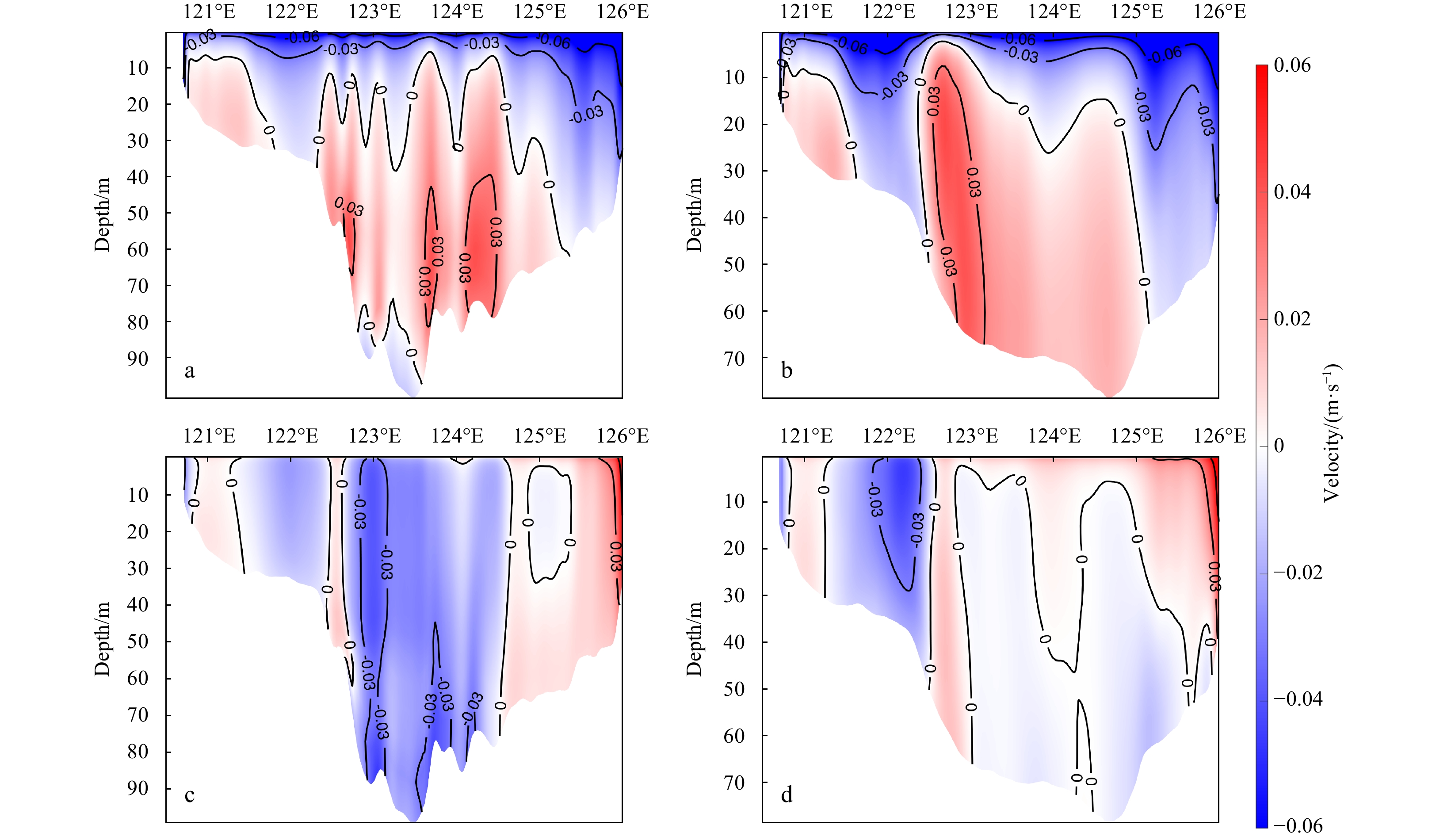
From the simulated results with the new revised bathymetry in the YS, we can find that the pattern of YSWC becomes more obvious, its speed increased significantly, and the unreasonable bending of its axis around 36.1°N, 123.5°E in the original system in winter disappeared (Fig. 2b). In order to qualitatively illustrate the effects of topography revision, the multi-year climatology mean meridional velocity across and along 36.15°N section in January are shown in Fig. 3. The meridional velocity with original topography shows three northward current cores located at the both sides of the YS trough, which located around 123.5°E, and weak southward current occurs at the bottom layer where water is deeper than 80 m. On the contrary, the northward meridional velocity with revised topography, occupies most of middle part of the section, and only one northward current core, with the speed larger than 2 cm/s, signing the axis of the YSWC is shown and located at about 123°E in the west of the YS trough, which is located about 124.8°E. For the zonal velocity along the section, it is about –2 cm/s for the case of unrevised topography, and almost 0 cm/s in the case of revised topography. As shown, the velocity field pattern of the YSWC is more obvious than before, and its flow axis moves westward to the range of longitude between 122.5°E and 123°E (Fig. 3b), which is consistent with the observation results of Yu et al. (2010) and Lin et al. (2011) and diagnostic computation results in previous literatures of Xu et al. (2005). The maximum value of climatology meridional velocity increases from 0.031 m/s to 0.034 m/s by about 11%.

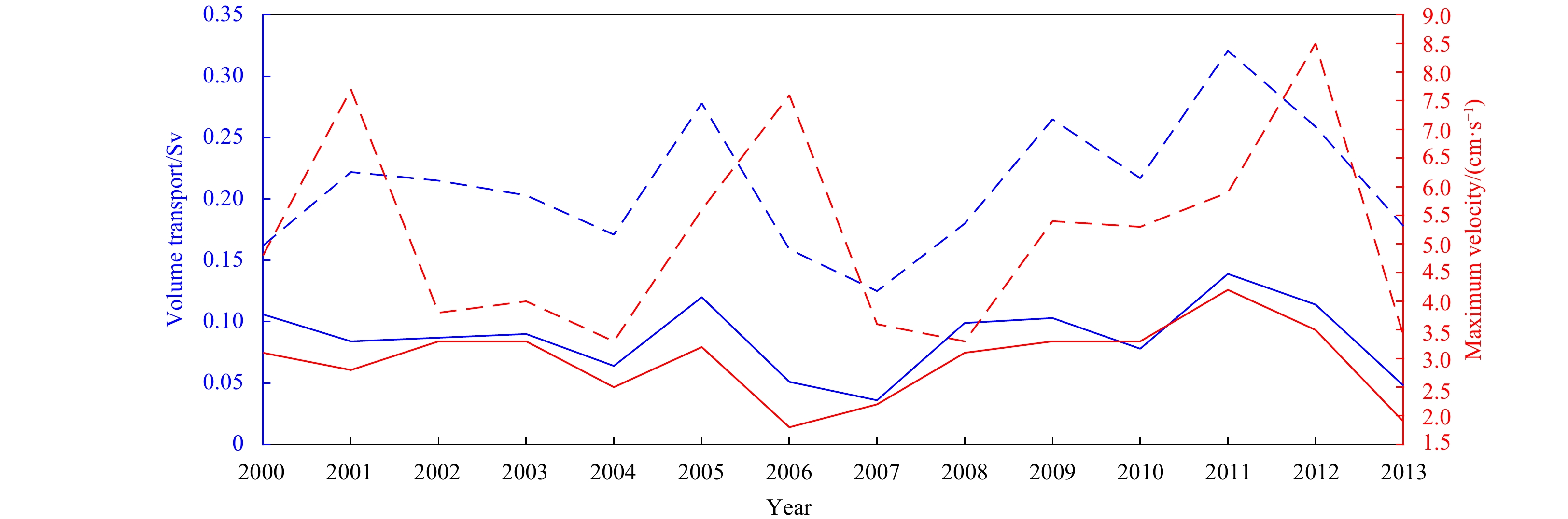
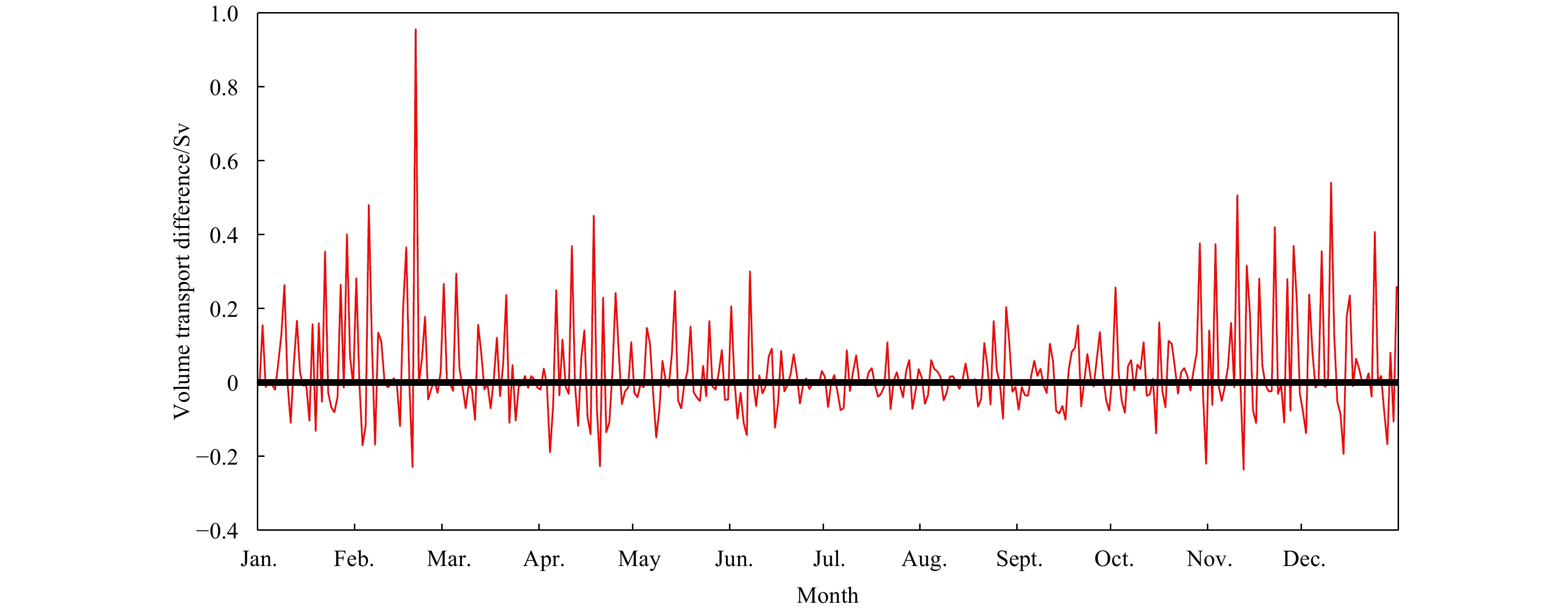
Furthermore, the yearly variations of monthly mean water volume transport (VT) and maximum meridional velocity across 35°N section in each January before and after the topography correction are quantitatively compared and shown in Fig. 4. Since the hindcast results of original system are simulated and archived only in 2000–2013, we just show the comparison between two systems during this period here. In winter, mean VT through 36°N section between 122°E and 124°E below 10 m area driven by YSWC increased from 0.08 Sv (1 Sv =106 m3/s) before the topography revised to around 0.17 Sv after the revision, with 122% increments. The maximum velocity of YSWC also increased significantly, from 0.026 m/s to 0.037 m/s on average, and the maximum velocity increased by about 41%. Both the qualitative analysis of the flow pattern of YSWC and quantitative analysis of its transportation show that the shape of YSWC is reproduced more obviously after the correction of topography.

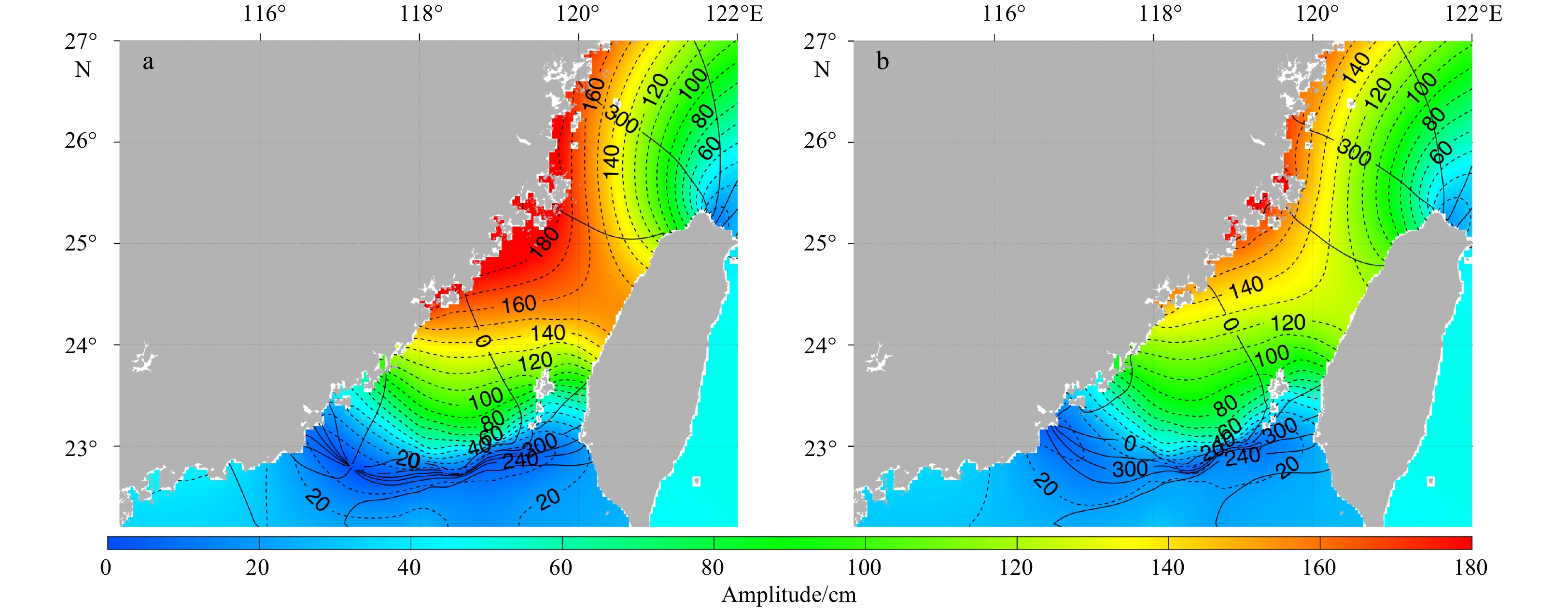
The accuracy of tidal simulation is also improved after the topography correction, concurrently. Taking M2 tidal constituent as an example, its amplitude still has an unreasonable amphidromic point in the southwest of the Taiwan Strait after the bathymetry revision (Fig. 5a). The maximum amplitude of M2 tidal constituent is over 180 cm in the middle-northern along the Fujian coast, and an unreasonable amphidromic point appears in the southwest of the Taiwan Strait and off shore Guangdong Province. In order to fix this problem, we conducted several sensitive experiments to modulate the model configuration by increasing bottom friction coefficient (BFC) in the Taiwan Strait. By changing the BFC from 2×10⁻³ to 1×10⁻² in the domain of the south 25.5°N and the west 120.9°E, we finally got the reasonable tidal distribution in the Taiwan Strait. The results show that after the BFC adjustment, the tidal amphidromic points of semi-diurnal constituents in this area disappear, amplitude decreases slightly to the reasonable range for the whole and around the Taiwan Strait. The simulated results (Fig. 5b) are more consistent with previous literatures (Fang et al., 1986).

By comparing the harmonic constants calculated from results before and after the correction with the analyzed results from the tide gauge data, which was used to validate the simulated results of tides in ECS area by Zhu and Liu (2012), it indicates that the absolute mean error of most harmonic constants of the four major tidal components (M2, S2, K1 and O1) have been decreased significantly, except that the amplitude of M2 and S2 components degraded slightly (Table 1).
| Tidal components | Harmonic constants | Absolute mean error | |
| Before | After | ||
| M2 | Amp/cm | 11.0 | 11.2 |
| Pha/(°) | 9.8 | 7.3 | |
| S2 | Amp/cm | 4.4 | 4.9 |
| Pha/(°) | 8.9 | 7.9 | |
| K1 | Amp/cm | 3.6 | 2.5 |
| Pha/(°) | 8.6 | 6.3 | |
| O1 | Amp/cm | 2.4 | 1.8 |
| Pha/(°) | 6.5 | 6.3 | |
 DownLoad:
CSV
DownLoad:
CSV
Sea surface atmospheric forcing is an important factor to heat, fresh water and momentum transferring between atmosphere and ocean, which could affect sea surface temperature, salinity and velocity field of modeling results. Therefore, it is also one of key elements to simulation accuracy of upper layer ocean states. Direct forcing using radiation flux fields and indirect forcing by calculating radiation flux fields using bulk-formulas (hereafter referred to as bulk_flux) of COARE3.0 (Fairall et al., 2003) are two common surface forcing modes used in many popular ocean models, i.e., ROMS, FVCOM (Finite Volume Community Ocean Model; Chen et al., 2013), NEMO and so on. Here, the direct surface forcing mode in the original system was replaced with the bulk_flux mode in the improving process, where the sea surface atmospheric forcing field is calculated and provided by the bulk-formulas using CFSR reanalysis data.
In COARE3.0, the calculation formulas for the air-sea fluxes, such as sensible heat, latent heat and long-wave radiation, are as follows:
| $$ {Q}_{s}={\rho }_{a}{C}_{p}{C}_{h}\left({T}_{s}-\theta \right){u}_{10}, $$ | (1) |
| $$ {Q}_{L}={\rho }_{a}{L}_{e}{C}_{e}\left({q}_{s}-{q}_{a}\right){u}_{10} ,$$ | (2) |
| $$ {Q}_{{\rm{longwave}}}={Q}_{{\rm{longwavedown}}}-\varepsilon {\sigma }_{sb}{T}_{s}^{4}, $$ | (3) |
where
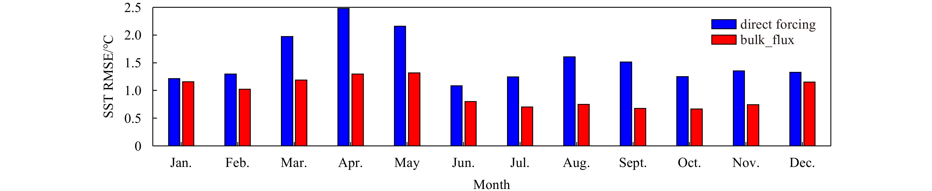
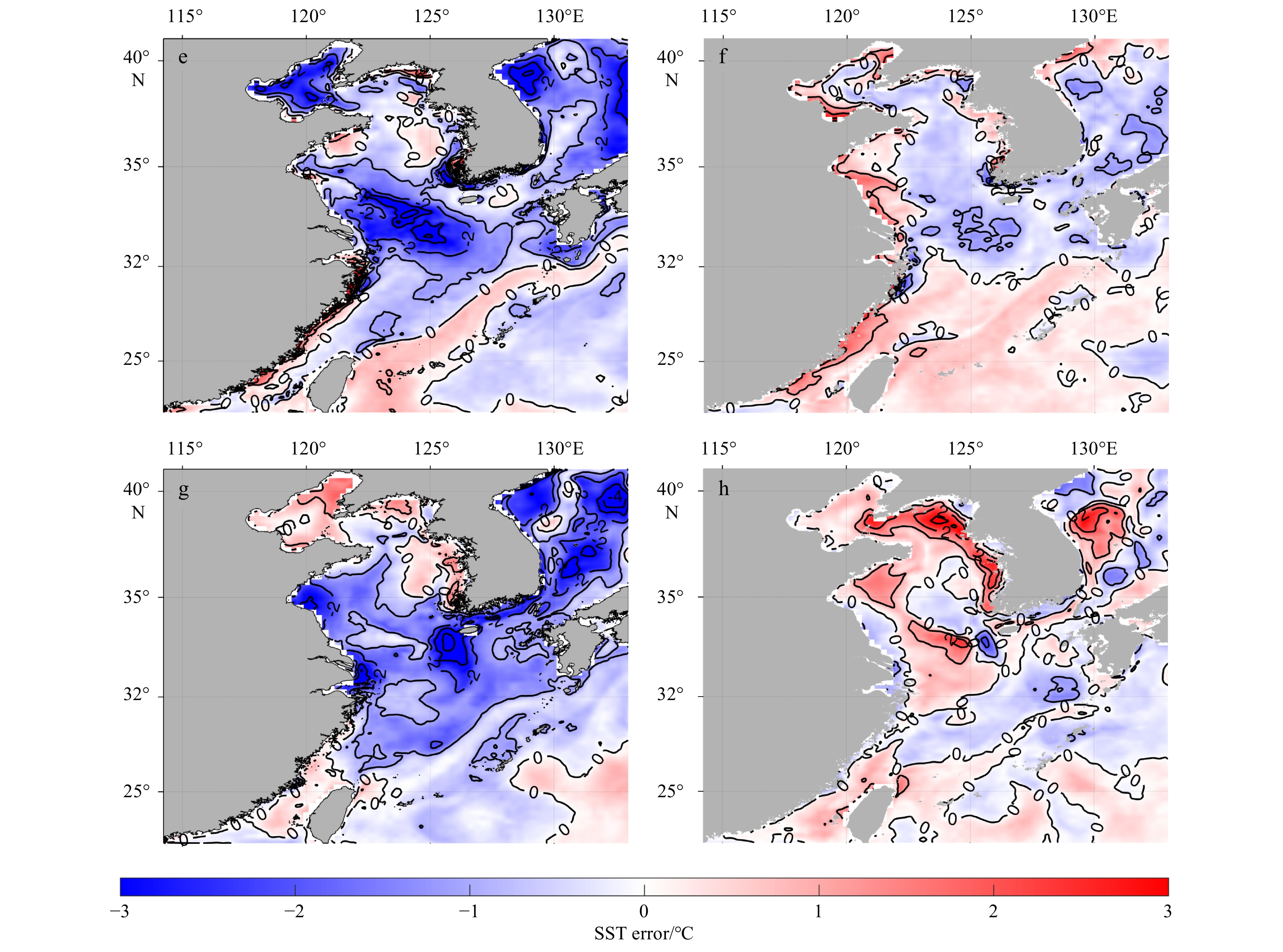
In order to evaluate the simulation results of two forcing modes, the simulated SSTs of the BYEOFS using direct forcing and bulk_flux mode were compared with the Merged Satellite and In-situ Data Global Daily SST (MGDSST) by calculating their deviations and root mean square errors (RMSE), respectively. To the simulated results in 2011, for example, the SST RMSE using bulk_flux mode was smaller than that of direct forcing obviously (Fig. 6) and RMSEs of monthly SST are all less than 1.5°C after using bulk_flux mode. Simulated results of SST in January, April, July and October are used to represent SST of winter, spring, summer and autumn, respectively. In winter, the SST RMSE of these two surface forcing modes are relatively close (Figs 7a, b) with a nearly 5% decreasing, while the simulation results using bulk_flux mode in spring, summer and autumn are distinctly better than direct forcing (Figs 7c–h). Especially in summer, the area where SST error above 2°C at western coastal area of BYES is almost absent. The reducing degrees of SST RMSE in these three seasons are all over 40% (48%, 44%, 47% in spring, summer and autumn, respectively). Monthly SST simulated using bulk_flux mode is closer to the observed SST. The reducing ratio of annual mean RMSE achieves 36%.


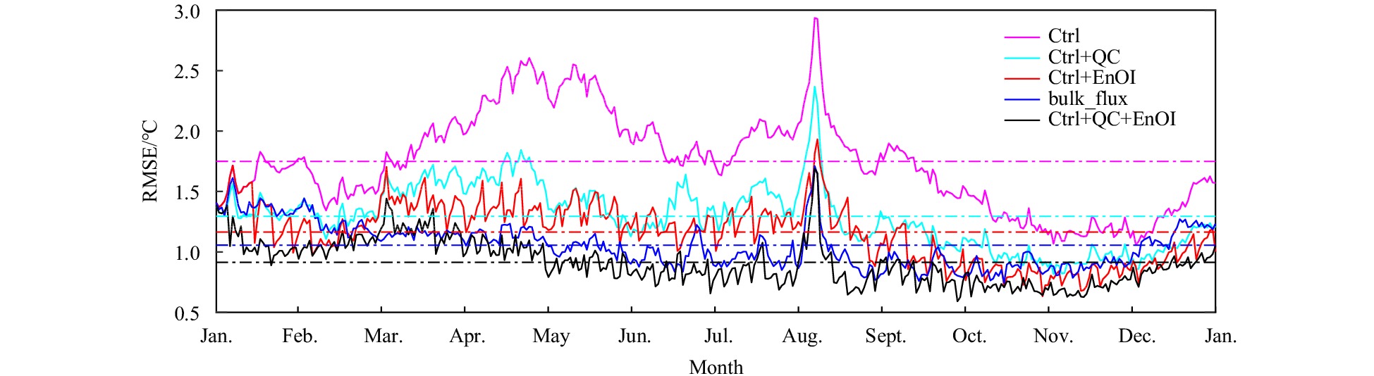
Further, simulated results of Ji et al. (2015), which includes the control-run simulation (Ctrl, Expt. 1), the control-run simulation added heat flux correction (Ctrl+QC, Expt. 2), the control-run simulation added EnOI assimilation (Ctrl+EnOI, Expt. 3), and control-run simulation added both heat flux correction and EnOI assimilation (Ctrl+QC+EnOI, Expt. 4) are compared with that from the bulk_flux mode (Expt. 5) to show effects of surface atmospheric forcing mode changing (Fig. 8). A more detailed setting of experiments is shown in Table 2. The annual mean RMSEs of SST of above five experiments are 1.75°C, 1.30°C, 1.16°C, 0.98°C and 1.06°C from Expt. 1 to Expt. 5, respectively. The simulated result of Expt. 5 on the annual mean RMSE (1.06°C) is closed to that (0.98°C) of Expt. 4, which the SST RMSE decreased by about 18% compared to the simulated result of Expt. 2 under the same settings for others. In terms of domain averaged RMSE of daily SST, the results of Expt. 5 are most close to the simulation results of Expt. 4 from March to October in 2011, and are similar to those of Expt. 2 and Expt. 3 in other months, although the results are slightly worse. It indicates that the improvement effect of simulated SST is closed to the effect of EnOI assimilation before the changing of surface forcing mode. Meanwhile, it is noted that the daily domain averaged results of Expt. 5 in 2011 are always better than those of Expt. 1. Those comparison experiments show that the change of surface forcing mode can significantly improve the simulation accuracy of SST.

| Test | Forcing mode | Correction | EnOI | Annual mean RMSE/°C |
| 1 | Direct forcing | × | × | 1.75 |
| 2 | Direct forcing | √ | × | 1.30 |
| 3 | Direct forcing | × | √ | 1.16 |
| 4 | Direct forcing | √ | √ | 0.98 |
| 5 | Bulk_flux | √ | × | 1.06 |
DownLoad:
CSV
For the simulation of model SST, the most direct and effective influence mode is the change of thermal radiation field on the sea surface, especially the change of net radiation flux. By comparing the difference distribution of three radiation fields generated by two forcing methods mentioned above (Figures not shown), it is found that latent radiation is the first major reason for different performances of SST simulation, and followed by the effect of sensible heat radiation difference (Li et al., 2019).
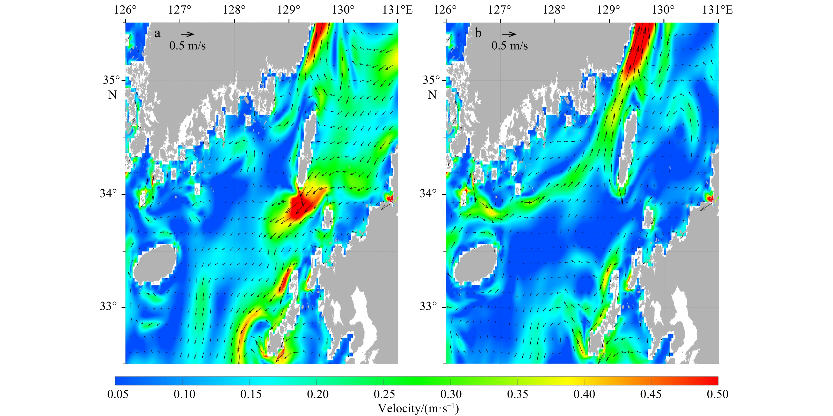
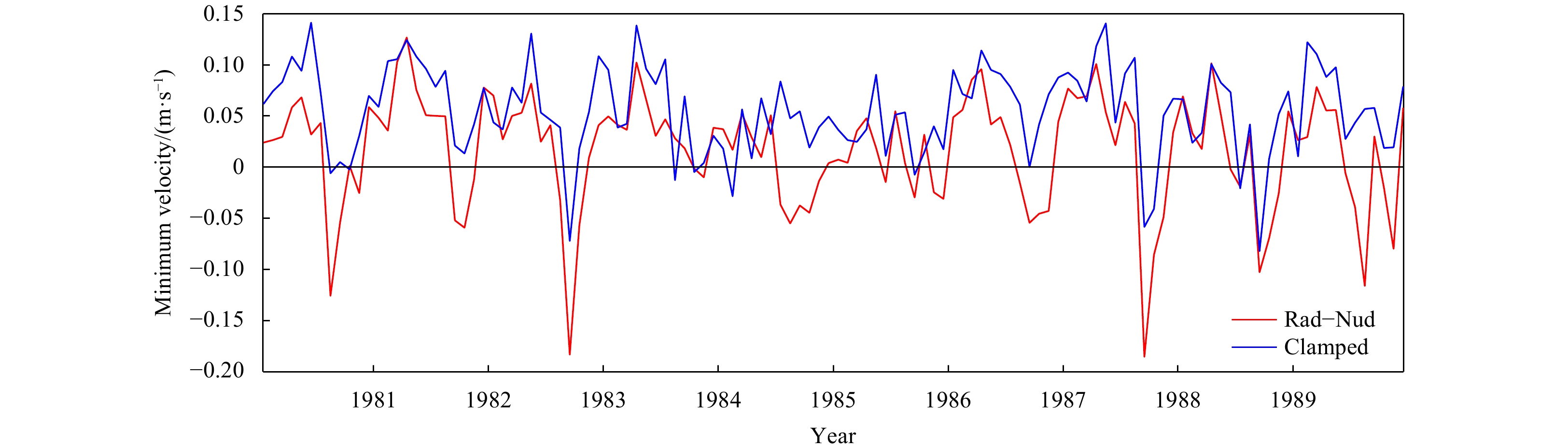
According to the historical observations, the mean flow of the TUS is northeastward into Japan Sea for year-round. The velocity in the eastern channel of TUS is mostly 0.26–0.51 m/s (Katoh, 1994), and time-averaged VT is 2.3–2.7 Sv across the TUS section (Teague et al., 2002) with maximum in early winter and minimum in early spring (Isobe, 1994). However, during the simulation and debugging process, it was found that a westward current appeared in the TUS (Fig. 9a), which was inconsistent with the actual situation. In order to get a better understanding on this problem, two sensitive experiments are conducted by employing two available open lateral boundary conditions in ROMS and applying to the eastern lateral boundary, the Clamped boundary condition (hereafter referred to as Clamped) (Shchepetkin and McWilliams, 2005) and the mixed radiation-nudging boundary condition (hereafter referred to as Rad-Nud) (Marchesiello et al., 2001). The Clamped is simply setting the boundary value to a known exterior value, while the Rad-Nud provides radiation condition on outflow and nudging to a known exterior value on inflow. Here both the outflow and the inflow are from SODA monthly mean datasets. When the Clamped option are used in eastern boundary condition, the outflow of the TUS almost disappeared (Fig. 9b), and the pattern of current tends to be reasonable. Further, the minimum of monthly normal flow through TUS section using Rad-Nud and Clamped boundary conditions was calculated respectively. The result shows that the velocity of negative normal flow decreases significantly in most months (Fig. 10).


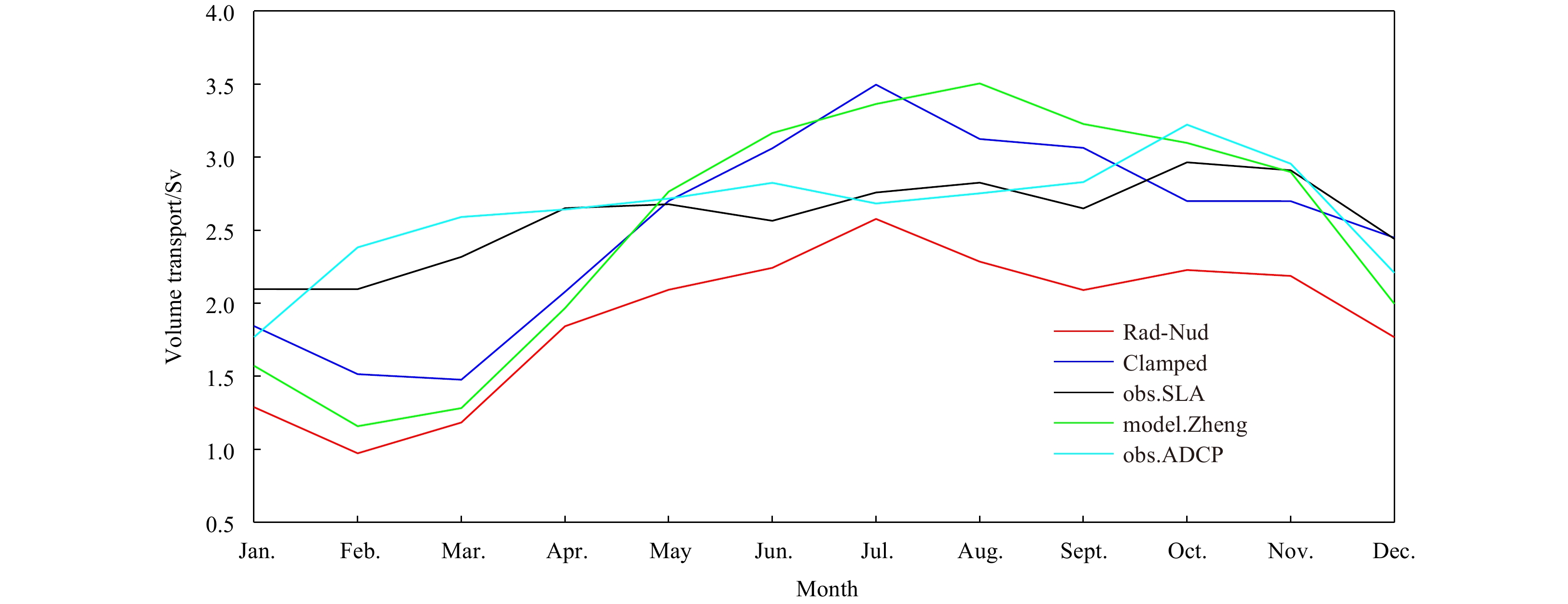
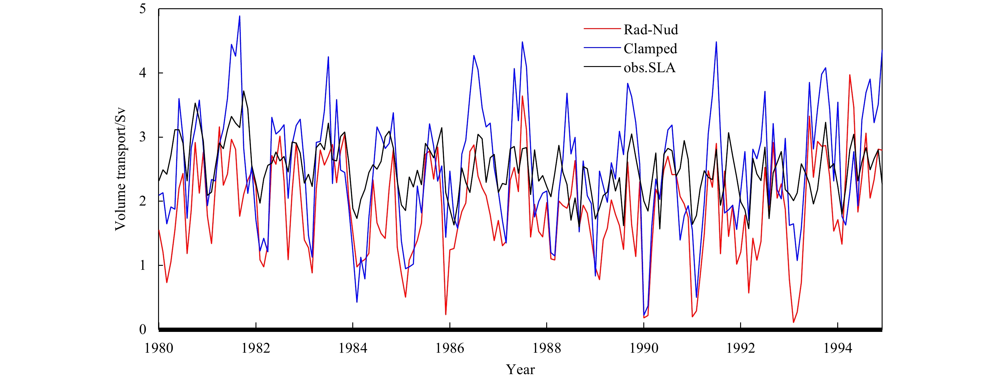
In order to verify the accuracy of Tsushima Strait Warm Current (TSWC) VT for the model after changing the eastern boundary condition from Rad-Nud to Clamped, the timeseries of monthly mean VT through the strait was calculated. We select the same section (35.07°N, 129.13°E–34.83°N, 129.49°E–33.73°N, 130.22°E) with Takikawa et al. (2005) to calculated the VT through TUS, the position for sections please refer to Fig. 1a in Takikawa et al. (2005). Compared with the results of Rad-Nud, when the Clamped boundary conditions were used in the system, climatology monthly mean VT through this strait was much closer to the ADCP observation (Takikawa et al., 2005), the flow rate calculated by SLA (Takikawa and Yoon, 2005) and the simulation results of Zheng et al. (2008) (Fig. 11). As shown in Table 3, the RMSE of VT through the TUS was reduced dramatically. A RMSE decrease was also detected by comparing the long-term time series of the monthly mean VT of the TSWC calculated by SLA data, dropping from 0.86 Sv to 0.79 Sv with the percentage of decreasing about 8.1% (Fig. 12). The absolute mean error decreases from 0.71 Sv to 0.65 Sv with the ratio about 8.4%. The results of climate state and monthly mean long-term variation of VT through TUS showed that the Clamped boundary conditions could improve the model skill of Tsushima Strait Warm Current.

| Observation type | Observations using ADCP/Sv | Calculated results using SLA/Sv | Model results of Zheng et al. (2008)/Sv |
| Clamped | 0.55 | 0.47 | 0.27 |
| Rad-Nud | 0.82 | 0.73 | 0.72 |
DownLoad:
CSV

As the use of radiation conditions alone without nudging to the external data is insufficient to keep model’s running stably, the adaptive nudging technique is used to handle the external information. To avoid blow-up and prevent substantial drift of simulation results during long-term integration, adaptive nudging layer has to be set in mixed Rad-Nud open boundary condition. The nudging layer is a region where a model data is relaxed towards external data. Although increasing stability of the system, the mixed Rad-Nud open boundary restrains the development of boundary flows at the same time. This character of Rad-Nud open boundary condition could be the reason for reducing eastward flow and generating the unreasonable westward flow.
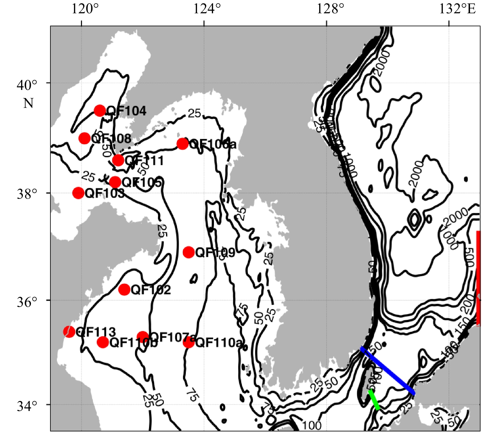
The monthly mean surface normal flow fields and VT through sections of TUS (34.3°N, 129.4°E–33.9°N, 129.7°E), the eastern channel of TUS (35.1°N, 129.1°E–34.2°N, 130.9°E) and the eastern lateral boundary (35.5°N, 133°E–37.3°N, 133°E) of the model domain (section positions shown in Fig. 13) were calculated to compare the influence of eastern boundary conditions. Once using Clamped condition at the eastern lateral boundary, the monthly mean VT in normal direction of these three sections increased significantly, and the number of months in which the abnormal negative flow basically cleared (blue line in Fig. 14).


The vertical distribution of normal velocity fields across three sections in December 1985 are compared, respectively (Fig. 15). All of them show in dramatically different current patterns under the Clamped and Rad-Nud boundary conditions. It is found that the normal flow component increased obviously along two sections, TUS and the eastern channel of TUS, while using Clamped condition, comparing with that from Rad-Nud condition being used. Especially at the TUS and its eastern channel sections (Figs 15a–d), the speed value of normal flow changes from most negative (westward) to positive (eastward). The maximum velocity speed values are over 0.2 m/s and 0.3 m/s for the TUS and its eastern channel, respectively. Meanwhile, along the eastern boundary position (Figs 15e, f), vertical distribution of the positive normal flow obtained by Clamped condition is also larger than that obtained by Rad-Nud condition.

By comparing the VT variations between through eastern lateral boundary and through the TUS, it is found that the VT through those two sections is significantly correlated with that through the eastern lateral boundary. The correlation coefficients of the VT between through the TUS and its eastern channel and through the eastern lateral boundary are 0.48 and 0.50 for the Rad-Nud condition, 0.59 and 0.61 for the Clamped condition, respectively, with an over 95% significance level. In addition, both correlation coefficients from Clamped condition are higher than those from Rad-Nud condition by about 0.11, which indicates a much stronger correlation between the currents through the eastern lateral boundary and the TSWC.
According to the suction effect of TSWC on the Taiwan Warm Current (Zheng et al., 2009), the flow field of eastern lateral boundary in the downstream area provides strong suction effect, which enhances the eastward current speed of TSWC. Compared with the Rad-Nud condition, the Clamped condition used the outflow information from SODA open boundary data directly, which could contribute to the velocity field of TUS and keep the positive flow direction more effectively.
As mentioned in Section 3.2, bulk_flux mode is used as a new sea surface atmospheric forcing calculation mode which taking the influence of mean sea level atmospheric pressure into account. In the meantime, it is found that atmospheric pressure could also exert an influence on the momentum equation. The atmospheric pressure can affect simulation results mainly by adding the horizontal mean sea level atmospheric pressure difference term to modify the pressure gradient force terms (Shchepetkin and McWilliams, 2003). There are two ways on which air pressure correction option influences the system results: the first one is correcting the baroclinic pressure gradient force term by adding the air pressure difference between the air pressure at mean sea level (
In order to check the influence of air pressure correction on simulation results, a pair of comparative experiments (with and without air pressure correction) was conducted to compare the variation of the sea level anomaly (SLA). Taking the simulation results in 2017 as an example, SLA of the YS in January (Figs 16a, b) and October (Figs 16g, h) decreased slightly, while that in April (Figs 16c, d) and July (Figs 16e, f) shows no obvious change after atmospheric pressure correction introduced into the system. To check the relationship between SLA and air pressure, air pressure difference of spatial distribution in these four months is calculated. The atmospheric pressure of YS is higher in winter and autumn, while the air pressure gradient is from the YS and the BS region to the western Pacific in these two seasons (Fig. 17). Larger atmospheric pressure gradient from the YS to the open sea results in more net outflow of sea water volume, then inducing the reduction of the sea surface height of YS. The pressure gradient in spring and summer is relatively small which cannot reduce the water exchange and SLA difference significantly.


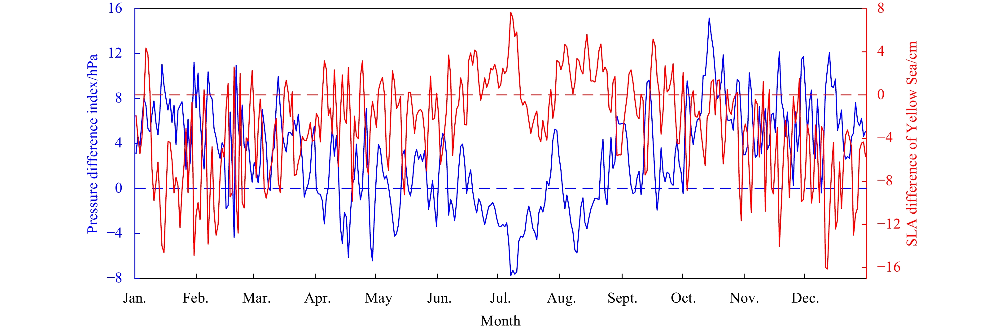
Further, according to the statistics of daily mean SLA in 2017, it is found that the daily mean SLA difference of YS area (north of 30°N, west of 127°E) between two experiments (with air pressure correction minus without air pressure correction) is most negative in winter and autumn and fluctuates around zero in spring and summer (red line in Fig. 18 ). The regional averaged difference of daily mean sea surface atmospheric pressure between the YS and area out of the YS was calculated and compared with the time series of regional averaged of SLA differences of the YS in these two experiments. The pressure difference shows the atmospheric pressure of the YS is higher in winter and autumn and fluctuates around zero in spring and summer (bule line in Fig. 18 ). It is found that the time series of mean air pressure difference and the mean SLA difference shows an obviously negative correlation, with the correlation coefficient is –0.60 and the confidence coefficient over 99%.

In winter, affected by cold snaps and air, mean sea level pressure in the YS and the BS is in an average state controlled by cold and high pressure system. According to the annual variation of air pressure, it is found that the daily mean sea level pressure in the model domain reaches its maximum value in winter, and the difference with the standard air pressure reaches its maximum, too (Fig. 18). The sea water pressure correction term affected by atmospheric pressure is basically positive in winter and decreases from the BS and the YS area to the ECS and surrounding sea area, resulting in the pressure gradient from the BS and the YS to the open sea area. The higher mean sea level air pressure in winter leads to an increase in the correction of pressure gradient forces.
The change of pressure gradient force finally affects the water exchange of the YS. By calculating the difference of daily mean VT through the 34.5°N section in these two tests, it is found that the absolute value of daily outflow (southward VT) from the YS is enhanced after considering mean sea level pressure correction, and the absolute difference (with air pressure correction minus without) of southward VT is significantly increased in winter (Fig. 19). The air pressure correction enhances water exchange between the YS and the ECS by increasing the outflow of the YS. The correlation analysis found that the outflow difference was significantly correlated with the atmospheric pressure, and the correlation coefficient was 0.23 with the confidence level over 99%. The pressure gradient forces outward open seas caused the outflow anomaly of the YS, then increasing the negative anomaly of sea level in the YS.

The analysis of SLA and air pressure shows that the addition of atmospheric pressure correction will increase the fluctuation of SLA by decreasing SLA of the YS in winter and autumn. In the meantime, the atmospheric pressure increases the rate of water exchange of the YS. The influence of this term on the simulation accuracy of SLA and coastal current field still needs further analysis after obtaining more accurate observed SLA and flow fields.
To validate BYEOFS’s improvements of forecasting skill in further, the optimum interpolation sea surface temperature (OISST) (Reynolds et al., 2007) and observation data from offshore in-situ 12 buoy stations in the BS and YS (red circles in Fig. 13) are employed to compare with BYEOFS forecasted SST for both before and after improvement, respectively. The forecasting experiments include 5 d forecasting results on the 1st, 11th and 21st days of each month in 2017. OISST is used to check the daily mean overall forecasting results, and in-situ buoy observations are used to check the hourly forecasting results.
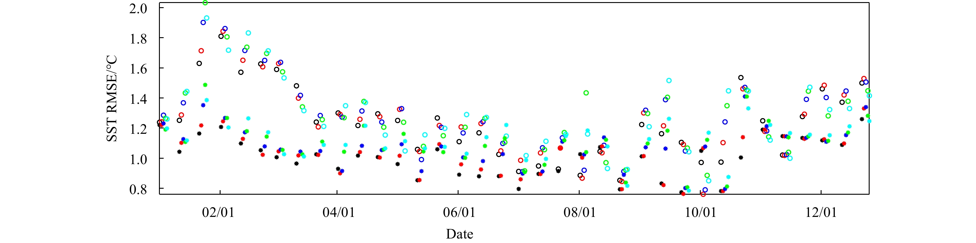
The annual mean RMSE of 5 d forecasting SST reduces from 1.24–1.30°C to 1.00–1.12°C after improving, with a significant reduction ratio of about 13%–19% (Table 4), by comparing with the OISST data. The mean value of SST RMSEs for all 5-day forecasting decreases from 1.27°C to 1.07°C after improving, with a decreasing ratio of 16% for SST forecasting skill. The RMSEs timeseries of domain averaged daily mean forecasted SST from the 1st to 5th day for before and after improving are shown in Fig. 20. It indicates that SST RMSE is reduced significantly after improving in boreal winter, but not in summer.
| 1st day | 2nd day | 3rd day | 4th day | 5th day | ||||||||||
| Before | After | Before | After | Before | After | Before | After | Before | After | |||||
| QF102 | 1.30 | 0.99 | 1.35 | 0.94 | 1.38 | 0.93 | 1.37 | 0.92 | 1.41 | 0.98 | ||||
| QF103 | 0.88 | 0.66 | 0.91 | 0.69 | 0.95 | 0.69 | 0.91 | 0.72 | 0.90 | 0.72 | ||||
| QF104 | 0.91 | 0.78 | 0.94 | 0.79 | 0.91 | 0.74 | 0.95 | 0.79 | 0.89 | 0.82 | ||||
| QF105 | 0.90 | 0.73 | 0.89 | 0.73 | 0.92 | 0.72 | 0.97 | 0.84 | 0.97 | 0.86 | ||||
| QF106a | 1.21 | 1.13 | 1.27 | 1.24 | 1.22 | 1.09 | 1.18 | 1.28 | 1.22 | 1.37 | ||||
| QF107a | 1.40 | 0.85 | 1.32 | 0.85 | 1.26 | 0.85 | 1.29 | 0.80 | 1.45 | 0.89 | ||||
| QF108 | 1.10 | 0.58 | 1.13 | 0.64 | 1.20 | 0.67 | 1.13 | 0.70 | 1.13 | 0.74 | ||||
| QF109 | 1.13 | 0.66 | 1.08 | 0.67 | 1.09 | 0.70 | 1.01 | 0.76 | 1.09 | 0.82 | ||||
| QF110a | 1.19 | 0.65 | 1.20 | 0.73 | 1.27 | 0.68 | 1.24 | 0.71 | 1.20 | 0.71 | ||||
| QF110b | 1.13 | 0.52 | 1.12 | 0.51 | 1.15 | 0.54 | 1.19 | 0.51 | 1.20 | 0.47 | ||||
| QF111 | 1.01 | 0.63 | 1.04 | 0.68 | 1.09 | 0.67 | 1.09 | 0.65 | 1.12 | 0.80 | ||||
| QF113 | 1.10 | 1.14 | 1.20 | 1.14 | 1.18 | 1.18 | 1.25 | 1.18 | 1.12 | 1.18 | ||||
| Average | 1.01 | 0.78 | 1.12 | 0.80 | 1.14 | 0.79 | 1.13 | 0.82 | 1.14 | 0.86 | ||||
DownLoad:
CSV

The annual mean RMSEs of hourly forecast SST for each forecasting day before and after improving by comparing with 12 buoy stations observation data are shown in Table 5. It is found that annual mean RMSEs at most buoy positions are significantly decreased. The averaged RMSEs of forecasting SST for all stations reduce from 1.01°C to 0.78°C, from 1.12°C to 0.80°C, from 1.14°C to 0.79°C, from 1.13°C to 0.82°C, from 1.14°C to 0.86°C, for the first to the fifth forecasting day, respectively. The overall reduction ratio ranges from 23% to 31% with a mean value 27% for all stations.
| Forecast day | 1st day | 2nd day | 3rd day | 4th day | 5th day |
| Before | 1.24 | 1.25 | 1.28 | 1.30 | 1.29 |
| After | 1.00 | 1.03 | 1.08 | 1.11 | 1.12 |
DownLoad:
CSV
In summary, the validation of SST RMSE shows that the forecasting skill of SST benefiting from the system’s improvements mentioned in above has improved dramatically.
The improvement of the BYEOFS represents the pattern of YSWC much better than BYEOFS-v1.0. Since the sea surface wind field data used in the system has not been changed, the correction of the model topography could be regarded as the principal factor for the improvement of the YSWC. Previous studies also found that the topography of the YS is an important factor affecting the axis location of YSWC. Lin and Yang (2011) found that the wind stress curl under the influence of V-shaped topography of YS is the primary cause of westward shift of YSWC. According to the traditional academic view about YSWC, it generally flows northward along the 50–70 m isobath of western side of YS trough (Guan, 1994; Tang et al., 2000). It was found that the depressions near 36.1°N and the discontinuous topography near 35.3°N in the west side of the YS (Fig. 2a) are the main differences between the two sets of topography data used in before and after system improving. The YSWC would bend its flow axis and lose its energy when it flows through above two areas. After the improvement of the topography, the area topography of the flow axis path is relatively smoother, resulting in the weakening of axis bending and energy loss.
In addition, uneven and speckled topography also exists in other areas of the YS trough, which may also affect the simulation of flow axis and velocity field of the YS in winter. The improvement of topography also reflects the importance of reasonable topography to the accuracy improvement of simulated velocity field. With the accumulation of oceanographic surveys data in the future, the model topography will be further modified to make it more realistic.
The accurate input of sea surface atmospheric forcing plays a key role in determining the model simulation result of SST. It is found from Eqs (1)–(3) in Section 3.2 that, by comparing with the direct forcing, the calculation of sensible heat flux, latent heat flux, and longwave radiation flux need to use SST from oceanic model. The increasing of SST can lead to the change of these three radiation fluxes, resulting in the increasing of sea surface heat loss, then inhibiting the continuous increasing of SST, vice versa. By introducing these calculation formulas, an effective negative feedback mechanism is formed between SST predicted by the ocean model and above three sea surface radiation fluxes field, which can effectively inhibit the abnormal warm or cold of SST in the system. Therefore, theoretically, the thermal radiation provided by bulk_flux mode is more reasonable and effective than direct forcing mode, especially for the case of the surface atmospheric forcing data with large errors (Li et al., 2019). Figure 7c shows the distributions of monthly mean SST differences of directly forcing mode minus MGDSST in April 2011. It is found that the simulated SST are much warmer than MGDSST near the coast areas of the BS, YS and Zhejiang Province. The maximum differences of SST mainly occur near the middle of BS, Subei shoal and the Changjiang Estuary, which are about 4–6°C. It is because sea surface atmospheric forcing data is not accurate, such as providing much more heat to ocean, which would manifest to heating the sea surface continually. This phenomenon can be alleviated significantly by employing the COARE 3.0 bulk algorithm which could introduce the effective negative feedback mechanism between model’s SST and air-sea heat flux into oceanic model. After changing the surface forcing mode, the maximum of monthly mean differences between simulated SST by bulk_flux and MGDSST are about 2–3°C, and the area of abnormal warmer SST is significantly reduced (Fig. 7d). It can be considered that in the case of large deviations in sea surface radiation flux data at the coastal area, the usage of bulk_flux mode can better ensure the accuracy of simulated SST.
However, the improvements to the BYEOFS-v1.0 presented in this paper mainly concern about sea surface temperature and patterns of mean velocity field or sea water volume transport. It is less related to three dimensional temperature and salinity structures or some specific physical processes, such water masses, the model or forecast skill in a typhoon process. Large number of in-situ observations are needed to support the exploration of influences of the vertical mixing schemes and turbulence parameterization by considering wave-induced mixing on the T/S profiles and vertical distribution of velocity based on BYEOFS-v2.0. Furthermore, the improvement of the data assimilation scheme allows assimilate much more observations from different platforms in subsurface layer, whose necessity has been widely acknowledged in many other coastal operational forecasting systems mentioned at the beginning. All in above will be our major direction to improve BYEOFS-v2.0 continually on the next step.
The BYEOFS based on ROMS has been upgraded and improved. The physical model configurations are modified in aspects such as correcting topography of the system, changing the surface forcing mode, adjusting the open boundary conditions, and using the mean sea level pressure correction option, and the simulation results are mainly compared. A set of comparison experiments are designed to distinguish different roles played by different model configuration in the upgrade process. Validated by observations and literature description, the simulated results show more consistence with the observations than before.
The axis of YSWC shows unreasonable bend around the 36.1°N area of the YS, influenced by inaccurate topography in BYEOFS-v1.0. The correction to system topography is by changing it to a combination of the GEBCO_08 bathymetric database and the measured bathymetric data of the BYES, which significantly improves the flow pattern of YSWC in winter. The velocity pattern of YSWC is more obvious and the unreasonable bending disappears after this correction.
With the change of surface atmospheric forcing from direct forcing mode to bulk_flux mode, sea surface radiation field of the system has built up a negative feedback relationship with model SST by employing the COARE 3.0 bulk algorithm. The change of surface atmospheric forcing remarkably improves the simulation and prediction ability of SST. The abnormal SST along the coastal area is significantly reduced. The annual mean RMSE of simulated SST after the improvement is 0.24°C less than that before the improvement, and the decreasing ratio is about 18%.
In the simulation and debugging process, it was found that a westward current in the TUS was inconsistent with the observations. The opening boundary conditions of eastern lateral boundary is adjusted from Rad-Nud to Clamped, which enhances the suction effect of eastern boundary. After this correction, the velocity of normal positive flow through the TUS significantly increased, and the abnormal westward flow rarely appeared.
Atmospheric pressure correction exerts an influence of sea level pressure on the momentum equation during the calculation process of the circulation model. The atmospheric pressure gradient from the YS and the BS region to the western Pacific will increase the fluctuation of SLA of the system in autumn and winter, while cold and high atmospheric pressure system affecting the region of YS. The mean sea level pressure correction option influences the outflow and SLA of YS area due to outward mean sea level pressure gradient in winter.
| [1] |
Bell M J, Schiller A, Le Traon P Y, et al. 2015. An introduction to GODAE OceanView. Journal of Operational Oceanography, 8(S1): s2–s11. doi: 10.1080/1755876X.2015.1022041
|
| [2] |
Chen Changsheng, Beardsley R C, Cowles G, et al. 2013. An Unstructured Grid, Finite-Volume Community Ocean Model FVCOM User Manual. 3rd ed. New Bedford: University of Massachusetts Dartmouth
|
| [3] |
Drévillon M, Greiner E, Paradis D, et al. 2013. A strategy for producing refined currents in the Equatorial Atlantic in the context of the search of the AF447 wreckage. Ocean Dynamics, 63(1): 63–82. doi: 10.1007/s10236-012-0580-2
|
| [4] |
Egbert G D, Erofeeva S Y. 2002. Efficient inverse modeling of barotropic ocean tides. Journal of Atmospheric and Oceanic Technology, 19(2): 183–204. doi: 10.1175/1520-0426(2002)019<0183:EIMOBO>2.0.CO;2
|
| [5] |
Evensen G. 2003. The Ensemble Kalman Filter: theoretical formulation and practical implementation. Ocean Dynamics, 53(4): 343–367. doi: 10.1007/s10236-003-0036-9
|
| [6] |
Fairall C W, Bradley E F, Hare J E, et al. 2003. Bulk parameterization of air-sea fluxes: updates and verification for the COARE algorithm. Journal of Climate, 16(4): 571–591. doi: 10.1175/1520-0442(2003)016<0571:BPOASF>2.0.CO;2
|
| [7] |
Fang Guohong, Zhao Baoren, Zhu Yaohua. 1991. Water volume transport through the taiwan strait and the continental skelf of the east china sea measured with current meters. Elsevier Oceanography Series, 54: 345–358. doi: 10.1016/S0422-9894(08)70107-7
|
| [8] |
Fang Guohong, Zheng Wenzhen, Chen Zongyong, et al. 1986. Analysis and Forecasting of Tides and Tidal Currents (in Chinese). Beijing: China Ocean Press
|
| [9] |
Graham R J, Gordon M, Mclean P J, et al. 2005. A performance comparison of coupled and uncoupled versions of the Met Office seasonal prediction general circulation model. Tellus A: Dynamic Meteorology and Oceanography, 57(3): 320–339. doi: 10.3402/tellusa.v57i3.14666
|
| [10] |
Guan Bingxian. 1994. Patters and structures of the currents in Bohai, Huanghai and East China Seas. In: Oceanology of China Seas. Kluwer Academic Publishers, 17–26
|
| [11] |
Guan Bingxian. 2002. Winter Counter-wind Current off the Southeastern China Coast (in Chinese). Qingdao: China Ocean University Press
|
| [12] |
Hellerman S, Rosenstein M. 1983. Normal monthly wind stress over the world ocean with error estimates. Journal of Physical Oceanography, 13(7): 1093–1104. doi: 10.1175/1520-0485(1983)013<1093:NMWSOT>2.0.CO;2
|
| [13] |
Hsueh Y, Wang J, Chern C S. 1992. The intrusion of the Kuroshio across the continental shelf northeast of Taiwan. Journal of Geophysical Research, 97(C9): 14323–14330. doi: 10.1029/92JC01401
|
| [14] |
Hu Dunxin, Ding Zongxin, Xiong Qingcheng. 1980. A preliminary investigation of cyclonic eddy in North East China Sea in summer. Chinese Science Bulletin, 25(1–2): 57–60
|
| [15] |
Isobe A. 1994. Seasonal variability of the barotropic and baroclinic motion in the Tsushima-Korea Strait. Journal of Oceanography, 50(2): 223–238. doi: 10.1007/BF02253481
|
| [16] |
Ji Qiyan, Zhu Xueming, Wang Hui, et al. 2015. Assimilating operational SST and sea ice analysis data into an operational circulation model for the coastal seas of China. Acta Oceanologica Sinica, 34(7): 54–64. doi: 10.1007/s13131-015-0691-y
|
| [17] |
Katoh O. 1994. Structure of the tsushima current in the southwestern Japan Sea. Journal of Oceanography, 50(3): 317–338. doi: 10.1007/–BF02239520
|
| [18] |
Kourafalou V H, De Mey P, Le Hénaff M, et al. 2015. Coastal Ocean Forecasting: system integration and evaluation. Journal of Operational Oceanography, 8(S1): s127–s146. doi: 10.1080/1755876X.2015.1022336
|
| [19] |
Le Kentang. 1984. A preliminary study of the path of the Changjiang dluted water: I. Model. Oceanologia et Limnologia Sinica (in Chinese), 15(2): 157–166
|
| [20] |
Le Kentang. 1989. A preliminary study of the path of the changjiang dluted water: II. The effect of local wind on the path. Oceanologia et Limnologia Sinica (in Chinese), 20(2): 139–148
|
| [21] |
Lea D, Mirouze I, King R, et al. 2015. The met office coupled atmosphere/land/ocean/sea-ice data assimilation system. In: EGU General Assembly 2015. Vienna, Austria: EGU
|
| [22] |
Li Ang, Zhang Miaoyin, Zhu Xueming, et al. 2019. A research on the optimal approach of CFSR surface flux data correction based on different surface forcing modes. Haiyang Xuebao (in Chinese), 41(11): 51–63
|
| [23] |
Lima J A M, Martins R P, Tanajura C A S, et al. 2013. Design and implementation of the Oceanographic Modeling and Observation Network (REMO) for operational oceanography and ocean forecasting. Revista Brasileira de Geofísica, 31(2): 209–228. doi: 10.22564/rbgf.v31i2.290
|
| [24] |
Lin Xiaopei, Yang Jiayan. 2011. An asymmetric upwind flow, Yellow Sea Warm Current: 2. Arrested topographic waves in response to the northwesterly wind. Journal of Geophysical Research, 116(C4): C04027. doi: 10.1029/2010JC006514
|
| [25] |
Lin Xiaopei, Yang Jiayan, Guo Jingsong, et al. 2011. An asymmetric upwind flow, Yellow Sea Warm Current: 1. New observations in the western Yellow Sea. Journal of Geophysical Research, 116(C4): C04026. doi: 10.1029/2010JC006513
|
| [26] |
Lü Xingang, Qiao Fangli, Xia Changshui, et al. 2010. Upwelling and surface cold patches in the Yellow Sea in summer: effects of tidal mixing on the vertical circulation. Continental Shelf Research, 30(6): 620–632. doi: 10.1016/j.csr.2009.09.002
|
| [27] |
Marchesiello P, McWilliams J C, Shchepetkin A. 2001. Open boundary conditions for long-term integration of regional oceanic models. Ocean Modelling, 3(1–2): 1–20. doi: 10.1016/S1463-5003(00)00013-5
|
| [28] |
Martin M J, Hines A, Bell M J. 2007. Data assimilation in the FOAM operational short-range ocean forecasting system: a description of the scheme and its impact. Quarterly Journal of the Royal Meteorological Society, 133(625): 981–995. doi: 10.1002/qj.74
|
| [29] |
Mehra A, Rivin I. 2010. A real time ocean forecast system for the North Atlantic Ocean. Terrestrial, Atmospheric and Oceanic Sciences, 21(1): 211–228. doi: 10.3319/tao.2009.04.16.01(iwnop)
|
| [30] |
Mo Dongxue, Hou Yijun, Li Jian, et al. 2016. Study on the storm surges induced by cold waves in the Northern East China Sea. Journal of Marine Systems, 160: 26–39. doi: 10.1016/j.jmarsys.2016.04.002
|
| [31] |
Oddo P, Adani M, Pinardi N, et al. 2009. A nested atlantic-mediterranean sea general circulation model for operational forecasting. Ocean Science, 5(4): 461–473. doi: 10.5194/os-5-461-2009
|
| [32] |
Reynolds R W, Smith T M, Liu Chunying, et al. 2007. Daily high-resolution-blended analyses for sea surface temperature. Journal of Climate, 20(22): 5473–5496. doi: 10.1175/2007JCLI1824.1
|
| [33] |
Saha S, Moorthi S, Pan Hualu, et al. 2010. The NCEP climate forecast system reanalysis. Bulletin of the American Meteorological Society, 91(8): 1015–1057. doi: 10.1175/2010BAMS3001.1
|
| [34] |
Shchepetkin A F, McWilliams J C. 2003. A method for computing horizontal pressure-gradient force in an oceanic model with a nonaligned vertical coordinate. Journal of Geophysical Research, 108(C3): 3090. doi: 10.1029/2001JC001047
|
| [35] |
Shchepetkin A F, McWilliams J C. 2005. The Regional Oceanic Modeling System (ROMS): A split-explicit, free-surface, topography-following-coordinate oceanic model. Ocean Modelling, 9(4): 347–404. doi: 10.1016/j.ocemod.2004.08.002
|
| [36] |
Shi Zhen, Li Xiang, Liu Na. 2016. Effects of different temporal resolution of wind and thermal forcing on simulated global ocean temperature. Marine Forecasts (in Chinese), 33(6): 1–9. doi: 10.11737/j.issn.1003-0239.2016.06.001
|
| [37] |
Storkey D, Blockley E W, Furner R, et al. 2010. Forecasting the ocean state using NEMO: The new FOAM system. Journal of Operational Oceanography, 3(1): 3–15. doi: 10.1080/1755876X.2010.11020109
|
| [38] |
Sun Xiangping, Xiu Shumeng. 1997. Analysis on the cold eddies in the sea area northeast of Taiwan. Marine Science Bulletin (in Chinese), 16(2): 1–10
|
| [39] |
Takikawa T, Yoon J H. 2005. Volume transport through the tsushima straits estimated from sea level difference. Journal of Oceanography, 61(4): 699–708. doi: 10.1007/s10872-005-0077-4
|
| [40] |
Takikawa T, Yoon J H, Cho K D. 2005. The tsushima warm current through Tsushima Straits estimated from ferryboat ADCP Data. Journal of Physical Oceanography, 35(6): 1154–1168. doi: 10.1175/jpo2742.1
|
| [41] |
Tang Yuxiang, Zou Emei, Lie H J, et al. 2000. Some features of circulation in the southern Huanghai Sea. Haiyang Xuebao (in Chinese), 22(1): 1–16. doi: 10.3321/j.issn:0253-4193.2000.01.001
|
| [42] |
Tang Yuxiang, Zou Emei, Lie H J. 2001. On the origin and path of the Huanghai Warm Current during winter and early spring. Haiyang Xuebao (in Chinese), 23(1): 1–12. doi: 10.3321/j.issn:0253-4193.2001.01.001
|
| [43] |
Teague W J, Jacobs G A, Perkins H T, et al. 2002. Low-frequency current observations in the Korea/Tsushima Strait. Journal of Physical Oceanography, 32(6): 1621–1641. doi: 10.1175/1520-0485(2002)032<1621:LFCOIT>2.0.CO;2
|
| [44] |
Tonani M, Balmaseda M, Bertino L, et al. 2015. Status and future of global and regional ocean prediction systems. Journal of Operational Oceanography, 8(S2): s201–s220. doi: 10.1080/1755876X.2015.1049892
|
| [45] |
Usui N, Ishizaki S, Fujii Y, et al. 2006. Meteorological Research Institute multivariate ocean variational estimation (MOVE) system: Some early results. Advances in Space Research, 37(4): 806–822. doi: 10.1016/j.asr.2005.09.022
|
| [46] |
Usui N, Wakamatsu T, Tanaka Y, et al. 2017. Four-dimensional variational ocean reanalysis: a 30-year high-resolution dataset in the western North Pacific (FORA-WNP30). Journal of Oceanography, 73(2): 205–233. doi: 10.1007/s10872-016-0398-5
|
| [47] |
Xu Dongyu, Liu Xiqing, Zhang Xunhua, et al. 1997. Geology of China Seas (in Chinese). Beijing: Geology Press
|
| [48] |
Xu Yi, Yu Fei, Zhang Zhixin, et al. 2005. Diagnostic computation of the Yellow Sea Warm Current in winter. Advances in Marine Science (in Chinese), 23(4): 398–407. doi: 10.3969/j.issn.1671-6647.2005.04.002
|
| [49] |
Yang Dezhou, Yin Baoshu, Liu Zhiliang, et al. 2012. Numerical study on the pattern and origins of Kuroshio branches in the bottom water of southern East China Sea in summer. Journal of Geophysical Research, 117(C2): C02014. doi: 10.1029/2011JC007528
|
| [50] |
Yang Dezhou, Yin Baoshu, Sun Junchuan, et al. 2013. Numerical study on the origins and the forcing mechanism of the phosphate in upwelling areas off the coast of Zhejiang province, China in summer. Journal of Marine Systems, 123–124: 1–18. doi: 10.1016/j.jmarsys.2013.04.002
|
| [51] |
Yu Fei, Zhang Zhixin, Diao Xinyuan, et al. 2010. Observational evidence of the Yellow Sea warm current. Chinese Journal of Oceanology and Limnology, 28(3): 677–683. doi: 10.1007/s00343-010-0006-2
|
| [52] |
Zhang Shuwen, Wang Qingye, Lü Yanhui, et al. 2008. Observation of the seasonal evolution of the Yellow Sea Cold Water Mass in 1996–1998. Continental Shelf Research, 28(3): 442–457. doi: 10.1016/j.csr.2007.10.002
|
| [53] |
Zheng Peinan, Wu Dexing, Lin Xiaopei. 2008. Simulation and analysis of shelf circulation and its seasonal variability in the tsushima strait. Periodical of Ocean University of China (in Chinese), 38(1): 7–16
|
| [54] |
Zheng Peinan, Bai Zhipeng, Wu Dexing, et al. 2009. The remote connection of the Taiwan and Tsushima warm currents. Haiyang Xuebao (in Chinese), 31(1): 1–9. doi: 10.3321/j.issn:0253-4193.2009.01.001
|
| [55] |
Zhu Xueming, Liu Guimei. 2012. Numerical study on the tidal currents, tidal energy fluxes and dissipation in the China Seas. Oceanologia et Limnologia Sinica (in Chinese), 43(3): 669–677
|
| 1. | Yinlin Zhu, Yuheng Wang, Liang Zhao. Research on the ensemble forecasting method for green tide paths in the Yellow Sea based on parameter perturbation. Marine Pollution Bulletin, 2025, 214: 117717. doi:10.1016/j.marpolbul.2025.117717 | |
| 2. | Hailun He, Benyun Shi, Yingjian Hao, et al. Forecasting sea surface temperature during typhoon events in the Bohai Sea using spatiotemporal neural networks. Atmospheric Research, 2024, 309: 107578. doi:10.1016/j.atmosres.2024.107578 | |
| 3. | Xueming Zhu, Ziqing Zu, Shihe Ren, et al. Improvements in the regional South China Sea Operational Oceanography Forecasting System (SCSOFSv2). Geoscientific Model Development, 2022, 15(3): 995. doi:10.5194/gmd-15-995-2022 | |
| 4. | Qingqing Pan, Siyu Lin, Wei Lu, et al. Space-Air-Sea-Ground Integrated Monitoring Network-Based Maritime Transportation Emergency Forecasting. IEEE Transactions on Intelligent Transportation Systems, 2022, 23(3): 2843. doi:10.1109/TITS.2021.3134838 |


Figures(21) / Tables(5)

Supported by:
Beijing Renhe Information Technology Co. Ltd

Ang Li, Xueming Zhu, Yunfei Zhang, Shihe Ren, Miaoyin Zhang, Ziqing Zu, Hui Wang. Recent improvements to the physical model of the Bohai Sea, the Yellow Sea and the East China Sea Operational Oceanography Forecasting System[J]. Acta Oceanologica Sinica, 2021, 40(11): 87-103. doi: 10.1007/s13131-021-1840-0

| Tidal components | Harmonic constants | Absolute mean error | |
| Before | After | ||
| M2 | Amp/cm | 11.0 | 11.2 |
| Pha/(°) | 9.8 | 7.3 | |
| S2 | Amp/cm | 4.4 | 4.9 |
| Pha/(°) | 8.9 | 7.9 | |
| K1 | Amp/cm | 3.6 | 2.5 |
| Pha/(°) | 8.6 | 6.3 | |
| O1 | Amp/cm | 2.4 | 1.8 |
| Pha/(°) | 6.5 | 6.3 | |
DownLoad:
CSV
| Test | Forcing mode | Correction | EnOI | Annual mean RMSE/°C |
| 1 | Direct forcing | × | × | 1.75 |
| 2 | Direct forcing | √ | × | 1.30 |
| 3 | Direct forcing | × | √ | 1.16 |
| 4 | Direct forcing | √ | √ | 0.98 |
| 5 | Bulk_flux | √ | × | 1.06 |
DownLoad:
CSV
| Observation type | Observations using ADCP/Sv | Calculated results using SLA/Sv | Model results of Zheng et al. (2008)/Sv |
| Clamped | 0.55 | 0.47 | 0.27 |
| Rad-Nud | 0.82 | 0.73 | 0.72 |
DownLoad:
CSV
| 1st day | 2nd day | 3rd day | 4th day | 5th day | ||||||||||
| Before | After | Before | After | Before | After | Before | After | Before | After | |||||
| QF102 | 1.30 | 0.99 | 1.35 | 0.94 | 1.38 | 0.93 | 1.37 | 0.92 | 1.41 | 0.98 | ||||
| QF103 | 0.88 | 0.66 | 0.91 | 0.69 | 0.95 | 0.69 | 0.91 | 0.72 | 0.90 | 0.72 | ||||
| QF104 | 0.91 | 0.78 | 0.94 | 0.79 | 0.91 | 0.74 | 0.95 | 0.79 | 0.89 | 0.82 | ||||
| QF105 | 0.90 | 0.73 | 0.89 | 0.73 | 0.92 | 0.72 | 0.97 | 0.84 | 0.97 | 0.86 | ||||
| QF106a | 1.21 | 1.13 | 1.27 | 1.24 | 1.22 | 1.09 | 1.18 | 1.28 | 1.22 | 1.37 | ||||
| QF107a | 1.40 | 0.85 | 1.32 | 0.85 | 1.26 | 0.85 | 1.29 | 0.80 | 1.45 | 0.89 | ||||
| QF108 | 1.10 | 0.58 | 1.13 | 0.64 | 1.20 | 0.67 | 1.13 | 0.70 | 1.13 | 0.74 | ||||
| QF109 | 1.13 | 0.66 | 1.08 | 0.67 | 1.09 | 0.70 | 1.01 | 0.76 | 1.09 | 0.82 | ||||
| QF110a | 1.19 | 0.65 | 1.20 | 0.73 | 1.27 | 0.68 | 1.24 | 0.71 | 1.20 | 0.71 | ||||
| QF110b | 1.13 | 0.52 | 1.12 | 0.51 | 1.15 | 0.54 | 1.19 | 0.51 | 1.20 | 0.47 | ||||
| QF111 | 1.01 | 0.63 | 1.04 | 0.68 | 1.09 | 0.67 | 1.09 | 0.65 | 1.12 | 0.80 | ||||
| QF113 | 1.10 | 1.14 | 1.20 | 1.14 | 1.18 | 1.18 | 1.25 | 1.18 | 1.12 | 1.18 | ||||
| Average | 1.01 | 0.78 | 1.12 | 0.80 | 1.14 | 0.79 | 1.13 | 0.82 | 1.14 | 0.86 | ||||
DownLoad:
CSV
| Forecast day | 1st day | 2nd day | 3rd day | 4th day | 5th day |
| Before | 1.24 | 1.25 | 1.28 | 1.30 | 1.29 |
| After | 1.00 | 1.03 | 1.08 | 1.11 | 1.12 |
DownLoad:
CSV
| Tidal components | Harmonic constants | Absolute mean error | |
| Before | After | ||
| M2 | Amp/cm | 11.0 | 11.2 |
| Pha/(°) | 9.8 | 7.3 | |
| S2 | Amp/cm | 4.4 | 4.9 |
| Pha/(°) | 8.9 | 7.9 | |
| K1 | Amp/cm | 3.6 | 2.5 |
| Pha/(°) | 8.6 | 6.3 | |
| O1 | Amp/cm | 2.4 | 1.8 |
| Pha/(°) | 6.5 | 6.3 | |
| Test | Forcing mode | Correction | EnOI | Annual mean RMSE/°C |
| 1 | Direct forcing | × | × | 1.75 |
| 2 | Direct forcing | √ | × | 1.30 |
| 3 | Direct forcing | × | √ | 1.16 |
| 4 | Direct forcing | √ | √ | 0.98 |
| 5 | Bulk_flux | √ | × | 1.06 |
| Observation type | Observations using ADCP/Sv | Calculated results using SLA/Sv | Model results of Zheng et al. (2008)/Sv |
| Clamped | 0.55 | 0.47 | 0.27 |
| Rad-Nud | 0.82 | 0.73 | 0.72 |
| 1st day | 2nd day | 3rd day | 4th day | 5th day | ||||||||||
| Before | After | Before | After | Before | After | Before | After | Before | After | |||||
| QF102 | 1.30 | 0.99 | 1.35 | 0.94 | 1.38 | 0.93 | 1.37 | 0.92 | 1.41 | 0.98 | ||||
| QF103 | 0.88 | 0.66 | 0.91 | 0.69 | 0.95 | 0.69 | 0.91 | 0.72 | 0.90 | 0.72 | ||||
| QF104 | 0.91 | 0.78 | 0.94 | 0.79 | 0.91 | 0.74 | 0.95 | 0.79 | 0.89 | 0.82 | ||||
| QF105 | 0.90 | 0.73 | 0.89 | 0.73 | 0.92 | 0.72 | 0.97 | 0.84 | 0.97 | 0.86 | ||||
| QF106a | 1.21 | 1.13 | 1.27 | 1.24 | 1.22 | 1.09 | 1.18 | 1.28 | 1.22 | 1.37 | ||||
| QF107a | 1.40 | 0.85 | 1.32 | 0.85 | 1.26 | 0.85 | 1.29 | 0.80 | 1.45 | 0.89 | ||||
| QF108 | 1.10 | 0.58 | 1.13 | 0.64 | 1.20 | 0.67 | 1.13 | 0.70 | 1.13 | 0.74 | ||||
| QF109 | 1.13 | 0.66 | 1.08 | 0.67 | 1.09 | 0.70 | 1.01 | 0.76 | 1.09 | 0.82 | ||||
| QF110a | 1.19 | 0.65 | 1.20 | 0.73 | 1.27 | 0.68 | 1.24 | 0.71 | 1.20 | 0.71 | ||||
| QF110b | 1.13 | 0.52 | 1.12 | 0.51 | 1.15 | 0.54 | 1.19 | 0.51 | 1.20 | 0.47 | ||||
| QF111 | 1.01 | 0.63 | 1.04 | 0.68 | 1.09 | 0.67 | 1.09 | 0.65 | 1.12 | 0.80 | ||||
| QF113 | 1.10 | 1.14 | 1.20 | 1.14 | 1.18 | 1.18 | 1.25 | 1.18 | 1.12 | 1.18 | ||||
| Average | 1.01 | 0.78 | 1.12 | 0.80 | 1.14 | 0.79 | 1.13 | 0.82 | 1.14 | 0.86 | ||||
| Forecast day | 1st day | 2nd day | 3rd day | 4th day | 5th day |
| Before | 1.24 | 1.25 | 1.28 | 1.30 | 1.29 |
| After | 1.00 | 1.03 | 1.08 | 1.11 | 1.12 |
 DownLoad:


 DownLoad: