

Figure
1.
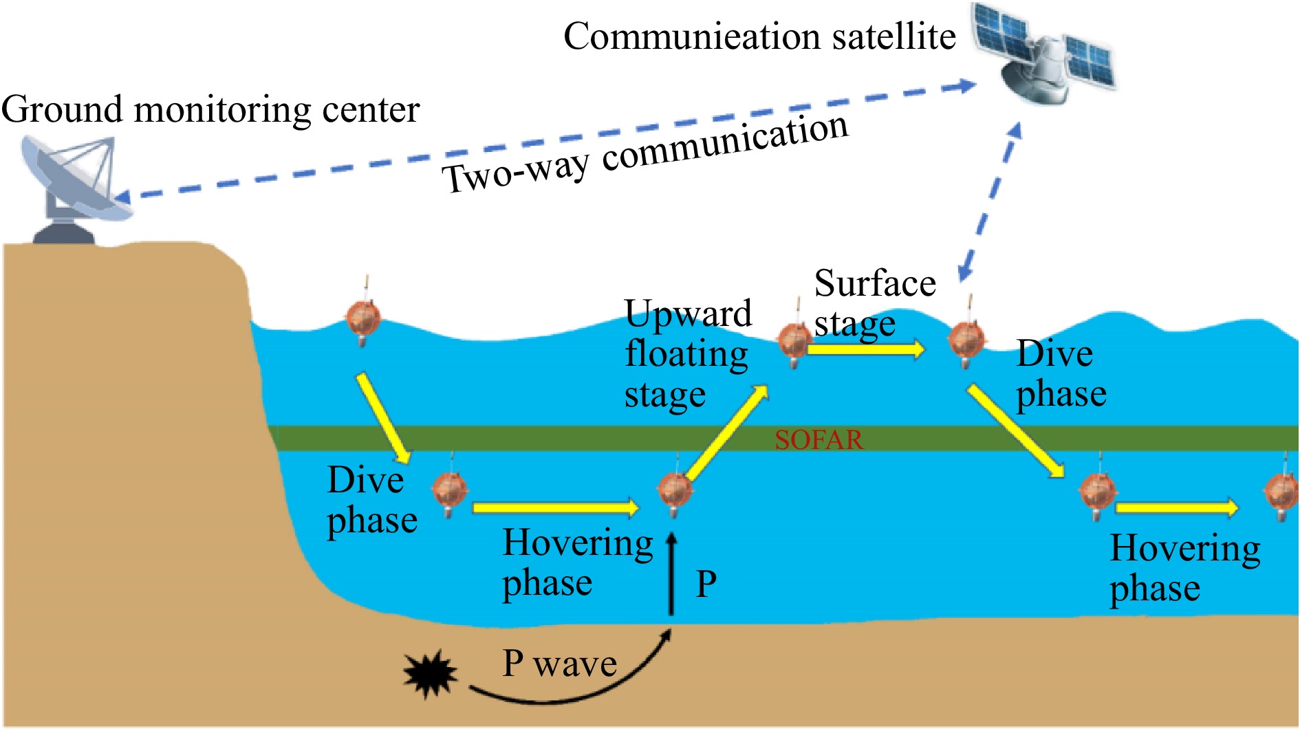
Schematic diagram of the operation of an MMS
| Citation: | Fei Hou, Jiabiao Li, Xinke Zhu, Weiwei Ding, Zhiteng Yu. A new fixed-depth suspension control algorithm for mobile marine seismometer and its testing results[J]. Acta Oceanologica Sinica.

|
Seismology was developed as a discipline in the 1889s and has since become an essential method for studying various aspects of Earth’s structure and geology, and it is based on a variety of data acquired by seismometers installed at seismic stations(Ben-Menahem, 1995). Thousands of permanent seismic stations have been operated on continental landmasses and islands, but few stations are located in the ocean, which covers nearly two-thirds of the area of the planet. This substantially restricts our understanding of the deep structure of the Earth under the oceans. Ocean-bottom seismometers (OBSs) are helpful instruments for collecting seismic data in the sea. However, OBSs are typically deployed for no more than one year due to their limited battery capacity. Furthermore, the high cost of delivery and recovery of OBSs also restricts their long-term uses, resulting in a significant lack of offshore seismic observation coverage, which has limited large/global-scale tectonic and structural studies(Tolstoy et al., 2006).
To overcome the problems mentioned above, the development of floating ocean seismometers started in late 1980(Joubert et al., 2015, 2016; Simon et al., 2021; Simons, 2021; Simons et al., 2009; Sukhovich et al., 2015), of which the typical representative is the Mobile Marine Seismograph (MMS), a vertical underwater vehicle. Compared to traditional fixed land-based seismic stations and OBSs, the MMSs can be suspended at a fixed depth, move with ocean currents, and transmit data via satellites, reducing the cost of seismic data recovery. MMSs can record signals conveyed by earthquakes (seismic P-waves) and thus are used to establish a seismic network covering an extensive marine area, solving the lack of long-term seismic stations in the oceans. In addition, the design lifespan of MMS exceeds three years, enabling the acquisition of additional seismic data, and is especially suitable for seismic tomography over large marine areas.
One of the critical operational requirements for an MMS is that it remains suspended at a desired depth for seismic monitoring for a specified time. Usually, the desired depth is ~1 500 m, below the axial depth of the deep ocean sound channel (SOFAR), ~
The Array for Real-time Geostrophic Oceanography (ARGO) buoy is another representative of the floating ocean instruments, and it has been widely deployed in the ocean. An ARGO buoy could measure seawater density using its onboard conductivity–temperature–depth (CTD) sensor to calculate the displacement volume required to hover at different depths. This capability enables rapid and precise fixed-depth hovering. However, this method for achieving constant depth hovering is unavailable due to the absence of a CTD sensor on MMS. Currently, research on the control technology of ocean observation equipment is based primarily on the proportional-integral-derivative (PID) algorithm and its various improvements (Carneiro et al., 2023; Hu et al., 2022; Huang et al., 2020; Keow et al., 2020; Ranganathan et al., 2020; Sholl et al., 2022). However, unlike autonomous underwater vehicles (AUVs), remotely operated vehicles (ROVs), and manned submersibles, most deep-sea self-powered MMSs are not equipped with peripheral feedback actuators such as thrusters, resulting in slow buoyancy change and vertical motion of the MMS (Gigacz et al., 2018; Poksawat et al., 2018; Sholl et al., 2022).
For the profile buoy, like an MMS that achieves vertical motion by changing buoyancy for ascent and descent, the system’s inertia affects the vertical movement of the float, resulting in a delayed response in the control process. Many studies have been extensively conducted on the fixed-depth control issues of such autonomous profiling floats. Barker (Barker, 2014) proposed a closed-loop control method that linearized a nonlinear model for a buoy depth-fixing control problem. However, in their study, oscillatory motion was observed when the float velocity was near zero, the motor restarted frequently, and the energy consumption for depth control was high, indicating that the equipment was unsuitable for long-term operation. Therefore, using conventional control methods like PID to control the self-sustaining profiling buoy will lead to a significant overshoot, steady-state system error, and frequent oil-pump motor action (Shi and Chad, 2014). In response to these problems, various depth control algorithms have been proposed ((Wang et al., 2022); (Qiu et al., 2020; Zhang et al., 2020)). Although the advanced algorithms exhibit delayed response and anti-interference capabilities, the model construction is complex, and the execution cost is high. In addition, these methods did not provide specific experimental validation, and the reliability and stability need further verification.
The MMS is a self-disposing device that carries limited onboard battery energy and must achieve a balance between the depth fixing and the cost of execution when executing fixed-depth suspension control. This study proposes a method of depth control for an MMS that addresses the issues of frequent buoyancy adjustments and high power consumption associated with PID and other control methods. The proposed method features fast convergence and efficient memory control, designed for fixed-depth adjustment while considering the constraints of inertia, delayed response, and limited battery energy.
An MMS consists of a protective case, a pressure-resistant compartment, an antenna, a hydrophone, a battery, and a buoyancy-adjustment mechanism (Fig. 2 (a)). The buoyancy-adjustment mechanism adjusts the net buoyancy of the MMS by changing the oil volume of the internal and external oil bladders, thereby controlling the ascent and descent of the MMS. During the descending stage, the MMS must overcome seawater density variations, dive to the preset operating depth, and adjust its net buoyancy through the fixed-depth suspension algorithm.

Force analysis of the MMS is required to intuitively analyze the vertical motion of an MMS during diving, suspension, and surfacing. A two-dimensional coordinate system is established with the depth measured in the vertical dimension as the coordinate Y-axis positive direction and any direction parallel to the sea surface as the X-axis positive direction. This study ignores the influence of the vertical component of the current on the motion of the MMS and the effect of seawater pressure on its shape change in order to simplify the state of motion analysis of the MMS. Because the pressure hull is made of glass material and has a slight deformation, the size of the MMS itself relative to its ascent and descent motion varies only very slightly, and the effect of the volume change can be ignored. The MMS is then subjected to the joint action of gravity (
a) Gravity
The MMS is subjected to gravity (
| $$ G=m\cdot g $$ | (1) |
Where
b) Buoyancy
The buoyancy force (
| $$ {F}_{\mathrm{f}}=-\rho \left(h\right)\cdot g\cdot V=-\rho \left(h\right)\cdot g\cdot \left({V}_{0}+V\left(\tau \right)\right) $$ | (2) |
Where
c) Resistance
Assuming that the MMS has a smooth form, its free fall in static seawater is subject to total resistance (
| $$ D=-\frac{1}{2}\rho \left(h\right){C}_{D}{v}^{2}A $$ | (3) |
Where
The combined forces of gravity determine the ascent and descent acceleration of the MMS, buoyancy, and drag as follows:
| $$ \sum F=G+{F}_{\mathrm{f}}+D=ma $$ | (4) |
Where
When the MMS floats on the sea surface, the vertical direction of motion speed
| $$ \rho \left(h\right)\cdot g\cdot \left({V}_{0}+V\left(\tau \right)\right)=m\cdot g $$ | (5) |
which gives
| $$ V\left(\tau \right)=\frac{m}{\rho \left(h\right)}-{V}_{0} $$ | (6) |
According to the high-pressure equation of state for seawater, the seawater density equation is obtained from the temperature, salinity, and pressure as follows:
| $$ \rho \left(S {\mathrm{,}}\; T {\mathrm{,}}\; P\right)=\dfrac{\rho \left(S {\mathrm{,}}\; T {\mathrm{,}}\; 0\right)}{1-\dfrac{P}{K\left(S {\mathrm{,}}\; T {\mathrm{,}}\; p\right)}} $$ | (7) |
| $$ \rho \left(S {\mathrm{,}}\; T {\mathrm{,}}\; 0\right)={\rho }_{w}+{A}_{1}S+{A}_{2}{s}^{\frac{3}{2}}+{A}_{3}{S}^{2} $$ | (8) |
Where
| Symbol | Value and Unit | Physical Significances | Symbol | Value and Unit |
Physical Significances |
| $ G $ | 514.515 N | The gravity force | $ D $ | N | The resistance force |
| m | 52.235 kg | The total mass of the MMS | $ v $ | m/s | The ascent and descent speeds of the MMS |
| $ g $ | 9.85 m/s2 | The acceleration due to gravity | $ \rho \left(h\right) $ | kg/m³ | The density of seawater at a depth of h m; |
| $ V $ | The volume of the external oil bladder | $ P $ | Pa | Seawater pressure | |
| $ A $ | 0.163 m2 | The cross-sectional area of the MMS. | $ T $ | ’℃ | Temperature |
| $ {V}_{0} $ | The initial drainage volume of the mms | $ S $ | ‰ | Salinity | |
| $ V\left(\tau \right) $ | The volume of the external oil bladder | $ a $ | m/s2 | the acceleration of the MMS |
|
| $ {F}_{f} $ | N | The buoyancy force |
 DownLoad:
CSV
DownLoad:
CSV
As derived in Section 2, seawater density and seawater pressure are one-to-one mapping functions. Considering that seawater pressure also corresponds uniquely to seawater depth h, seawater density at different depths also corresponds uniquely to seawater depth. Then, it is known that MMSs with varying volumes of drainage will be suspended at different seawater densities related to seawater depth without considering the influence of currents.
The algorithm’s core is to employ a binary search method to quickly and accurately determine the appropriate displacement volume based on the seismometer’s depth and vertical velocity, thereby enabling fixed-depth hovering. The device relies solely on buoyancy changes for vertical movement, which leads to a significant time delay in the control system. This study analyzes the motion trends of the seismometer and establishes two boundary conditions for buoyancy control to prevent excessive adjustments that could result in oscillations and increased energy consumption.
Once fixed-depth hovering is achieved, the algorithm records the current buoyancy value to reference future depth control. Given that the device’s drift distance during a single operational cycle is limited and seawater density remains relatively stable, utilizing this reference value reduces the number of buoyancy adjustments required. This approach facilitates faster depth stabilization, lowers energy consumption, and extends the device’s lifespan.
Suppose that the real-time depth of the MMS is

Therefore, when the buoyancy control system starts to find
Because the changes in the buoyancy and vertical motion of the MMS are slow and influenced by the inertia of the system, a response time lag exists in the control process. Therefore, to improve the control effect, it is necessary to analyze the fluctuation in the vertical motion of the MMS to avoid an invalid buoyancy adjustment. As shown in Fig. 4, even if the MMS exceeds the upper and lower boundaries of the fixed-depth range for a short time, it is feasible to complete the fixed-depth suspension gradually. Therefore, the relationship between

In the process of controlling the MMS to suspend at a fixed depth, if the effect of the vertical component of the current motion is not considered when the buoyancy of the MMS is adjusted to the suspension buoyancy interval

1) Fixed step to find a fixed-depth buoyancy interval
Before the first k buoyancy adjustments are completed, the vertical motion trend of the MMS remains unchanged (Fig. 5), meaning that the buoyancy of the MMS always has
2) Determine the fixed-depth buoyancy interval
When the kth buoyancy adjustment is completed (
3) Rapid convergence into a constant-depth buoyancy interval
To quickly converge the buoyancy of the MMS into
The MMS adjusts its negative buoyancy to its maximum value at the beginning of the dive to achieve the highest speed. When the MMS dives to the upper boundary of the preset suspension depth range (i.e.,
After completing the initial buoyancy adjustment, if the MMS is suspended within the preset operational depth range and shows fluctuation in depth at a speed less than the preset value, the MMS is considered to be in a suspended state; however, if the MMS exceeds the operational depth range and triggers the buoyancy adjustment condition, it is adjusted according to the neutral buoyancy adjustment mechanism in Fig. 6 until it meets the suspended state. After entering the suspended state, the MMS detects its depth change at a fixed frequency (usually set to 10 min); if the adjustment condition is triggered, it is adjusted according to the adjustment scheme shown in Fig. 6 to ensure that the MMS retains the suspended state. The pseudocode for the algorithm execution is shown in Table 2.

| Input: the real-time depth of the MMS is $ d $, the suspension depth is $ H $, the allowable depth fluctuation during the suspension is $ \Delta H $, the hovering speed $ {v}_{h} $, the previous suspension state $ {V}_{p} $, the first k buoyancy adjustments $ {q}_{k} $. Output: displacement volume $ V $ |
| 1. $ V={V}_{p} $ |
| 2. if $ d < (H-\Delta H) $ && Trigger adjustment |
| 3. { |
| 4. if Determination($ {q}_{k} $) { //whether the oil drain adjustment |
| 5. $ {q}_{k}={q}_{k}/2 $} |
| 6. $ \text{V}=V-{q}_{k} $ |
| 7. } else if d > (H +∆H) && Trigger adjustment |
| 8. { |
| 9. if Determination($ {q}_{k} $) { //whether the oil return adjustment |
| 10. $ {q}_{k}={q}_{k}/2 $} |
| 11. $ \text{V}=V+{q}_{k} $ |
| 12.} |
| 13. else { |
| If speed < the set value |
| 14. hover |
| 15.} |
DownLoad:
CSV
To achieve a fast and accurate determination of the required displacement volume for hovering, a method similar to the "bisection method" for root finding was employed. The displacement volume range was gradually narrowed until it approached the value of
If
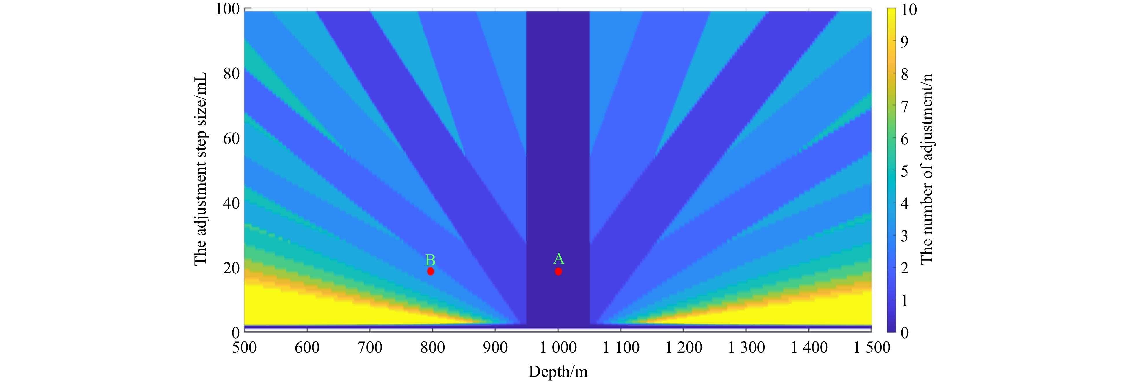
The convergence speed of the fixed-depth algorithm was influenced by variations in the seawater density, target fixed-depth value, range of fixed-depth control, and adjustment of oil quantity. Using actual measured seawater density data from the South China Sea (Fig. 7), we analyzed the convergence speed of the fixed-depth control algorithm. Assuming a target fixed depth of

| $$ \rho \left(d\right)=4.581\times {10}^{-10}{d}^{3}-2.4105\times {10}^{-6}{d}^{2}+0.0089479d+1025.0285 $$ | (9) |
The simulation results are shown in Fig. 8. Point A represents the scenario in which, after the initial buoyancy adjustment, the device can hover at a depth of 989 m with zero adjustment iterations, achieving the desired hovering state. Point B represents the scenario in which, after the initial buoyancy adjustment, the device can hover at a depth of 800 m, requiring three adjustment iterations for the control algorithm to achieve the necessary buoyancy for hovering. The simulation results indicated that the number of adjustment iterations decreased as the adjustment step size increased. However, larger adjustment step sizes result in longer pump activation, leading to energy wastage. When the adjustment step size exceeded 20 ml, a further increase in the step size did not significantly reduce the number of adjustment iterations. Therefore, a step size of 20 ml was used in this study. Even with more significant errors (500 m), hovering was achieved through six adjustment iterations. The analysis demonstrated that the algorithm has a theoretically fast convergence speed when selecting an appropriate adjustment for the oil volume.
According to Eq. (6), (7), and (9), a one-to-one mapping relationship exists between the displacement volume of the mobile marine seismometer and the depth of the hover. The relationship between the displacement volume
| $$ \begin{split}\frac{m}{{V}_{0}+V\left(\tau \right)}=& 4.581\times {10}^{-10}{H}^{3}-2.4105\times {10}^{-6}{H}^{2}+\\ & 0.0089479H+1025.0285 \end{split}$$ | (10) |
Where

A sea trial of the MMSs was conducted in the South China Sea starting in April 2021. The trial was executed in a sea area with a radius of 50 nautical miles centered on 17°46.9ʹN, 114°24.1ʹE, and the average water depth of the trial area was greater than

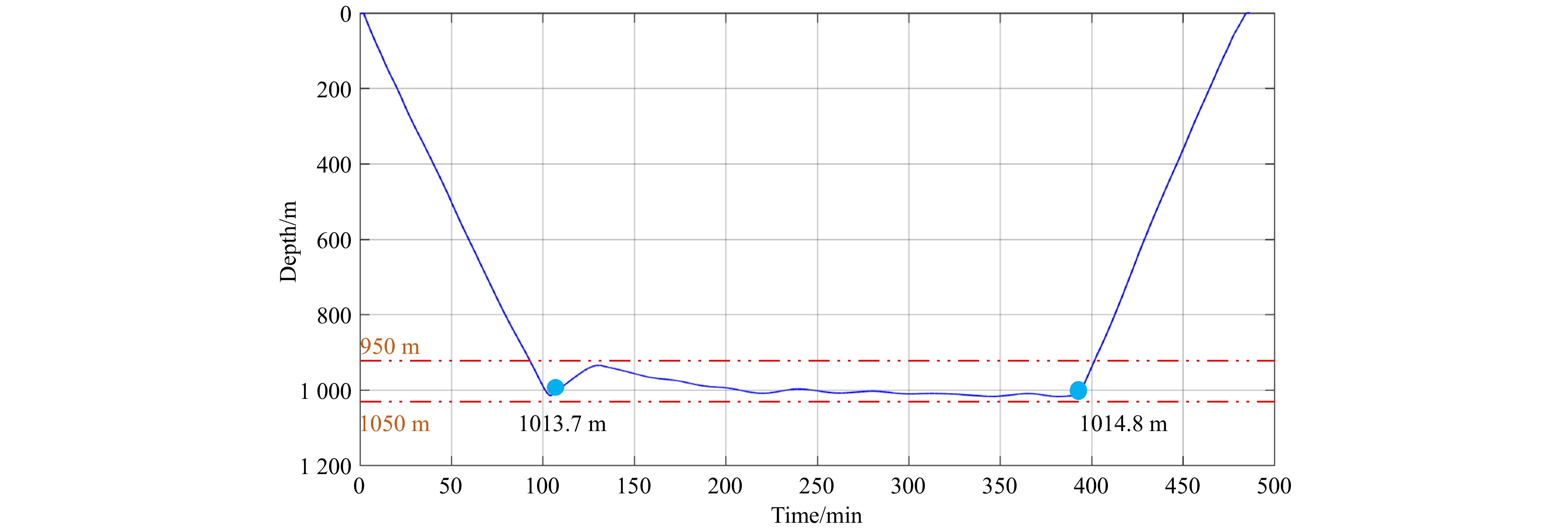
The short-term trial (Fig. 10b) parameters were set as follows: a suspension depth fixed at
The vertical profiles of the other MMSs involved in the short-term trial are presented in Fig. 12. MMS No-12 and No-16 were set to a fixed depth of 500m, and the rest of the MMSs were set to a fixed depth of 1000m. The depth curves show that different seismometers can be suspended relatively quickly after a short adjustment period. The short-term trial shows that the fixed-depth control algorithm designed in this study could achieve an MMS fixed-depth suspension with fewer buoyancy adjustments (less than four times on average during the experiment) and better suspension control in the case of unknown seawater density.

Based on the results of the short-term trial, the two MMSs were placed in the trial area for a 3-month-long applicability trial to verify their overall operating performance. The MMSs were recovered in early August 2021. During the trial period, the two MMSs were operated for 95 d, with 44 cycles and 532 nautical miles of travel. The MMSs were 258 nautical miles apart at the time of recovery. The drift tracks of the two MMSs are shown in Fig. 10c.
The parameters of this trial were set as follows: a suspension depth of 800 m, an allowable vertical fluctuation range of ±100 m, and an entry of the MMS into the suspension state at a speed of <0.01 m/s. The dive duration of the MMSs gradually increased over time (Fig. 13 (a)). The blue curve represents the operating time of MMS No-12 across various dive cycles. The first ten dives had shorter durations, averaging 55 hours, while the last 12 dives were extended to 6.5 days. The red curve indicates the operating time of MMS No-13. An analysis of the operating status of the MMS for three months showed that the MMSs were in a fixed-depth suspension state 98% of the time(Fig. 13 (b)), indicating that the fixed-depth control algorithm can realize MMS long-term fixed-depth suspension and reduce the influence of ocean currents, enabling the MMS to record seismic events.

As shown in Fig. 14 (a) and Fig. 15(a), as the number of MMS dives increased, the overall number of starts of the fixed-depth suspension control algorithm decreased. The average number of adjustments was reduced by about 10. At a depth of 800 meters underwater, the energy consumption for a single buoyancy adjustment of the seismometer is 0.067 Wh, resulting in a total energy savings of 0.67 Wh per profile. Through semi-physical simulation testing, the device’s power consumption for a single operational cycle (7 days) was 27 Wh, with an energy savings of 2.5%. Based on the device’s designed lifespan of 3 years, the algorithm can save 105 Wh compared to the initial adjustment, extending the operational period by 3.9 cycles. Also, as shown in Fig. 14 (b) and 15 (b), the MMSs can achieve a satisfactory effect in long-term operations, with an average suspension depth of 765.4 m in the long-term trial and an average drift depth of 29.6 m. The long-term trial showed that the fixed-depth suspension algorithm designed in this study can effectively and efficiently control an MMS to achieve a fixed-depth suspension and that the maintenance of the position of the MMS within the suspension zone is also satisfactory.


In this study, we addressed the problem of fixed-depth suspension control for a mobile marine seismometer with a limited onboard energy supply. We developed an effective fixed-depth control algorithm with a low depth adjustment cost that does not depend on seawater density data by establishing an MMS motion model and analyzing the fluctuations in vertical motion. Sea trials demonstrated that the control algorithm produced a satisfactory fixed-depth suspension, maintained the desired fixed depth, and mitigated the influence of ocean currents without requiring complex computations or hydrodynamic analysis of the MMS.
The algorithm’s simplicity and low computational requirements make it suitable for drifting buoys like the MMS, which rely solely on buoyancy adjustments for vertical motion. This innovative approach provides a new avenue for the fixed-depth control of other deep-sea equipment that utilizes buoyancy adjustments via an oil bladder, enhancing performance without complex control systems. Additionally, the algorithm has a memory function that allows for faster subsequent depth adjustments, reducing the number of corrections, lowering energy consumption, and extending the operational lifespan of the equipment.


Supported by:
Beijing Renhe Information Technology Co. Ltd

Fei Hou, Jiabiao Li, Xinke Zhu, Weiwei Ding, Zhiteng Yu. A new fixed-depth suspension control algorithm for mobile marine seismometer and its testing results[J]. Acta Oceanologica Sinica.

| Symbol | Value and Unit | Physical Significances | Symbol | Value and Unit |
Physical Significances |
| $ G $ | 514.515 N | The gravity force | $ D $ | N | The resistance force |
| m | 52.235 kg | The total mass of the MMS | $ v $ | m/s | The ascent and descent speeds of the MMS |
| $ g $ | 9.85 m/s2 | The acceleration due to gravity | $ \rho \left(h\right) $ | kg/m³ | The density of seawater at a depth of h m; |
| $ V $ | The volume of the external oil bladder | $ P $ | Pa | Seawater pressure | |
| $ A $ | 0.163 m2 | The cross-sectional area of the MMS. | $ T $ | ’℃ | Temperature |
| $ {V}_{0} $ | The initial drainage volume of the mms | $ S $ | ‰ | Salinity | |
| $ V\left(\tau \right) $ | The volume of the external oil bladder | $ a $ | m/s2 | the acceleration of the MMS |
|
| $ {F}_{f} $ | N | The buoyancy force |
DownLoad:
CSV
| Input: the real-time depth of the MMS is $ d $, the suspension depth is $ H $, the allowable depth fluctuation during the suspension is $ \Delta H $, the hovering speed $ {v}_{h} $, the previous suspension state $ {V}_{p} $, the first k buoyancy adjustments $ {q}_{k} $. Output: displacement volume $ V $ |
| 1. $ V={V}_{p} $ |
| 2. if $ d < (H-\Delta H) $ && Trigger adjustment |
| 3. { |
| 4. if Determination($ {q}_{k} $) { //whether the oil drain adjustment |
| 5. $ {q}_{k}={q}_{k}/2 $} |
| 6. $ \text{V}=V-{q}_{k} $ |
| 7. } else if d > (H +∆H) && Trigger adjustment |
| 8. { |
| 9. if Determination($ {q}_{k} $) { //whether the oil return adjustment |
| 10. $ {q}_{k}={q}_{k}/2 $} |
| 11. $ \text{V}=V+{q}_{k} $ |
| 12.} |
| 13. else { |
| If speed < the set value |
| 14. hover |
| 15.} |
DownLoad:
CSV
| Symbol | Value and Unit | Physical Significances | Symbol | Value and Unit |
Physical Significances |
| $ G $ | 514.515 N | The gravity force | $ D $ | N | The resistance force |
| m | 52.235 kg | The total mass of the MMS | $ v $ | m/s | The ascent and descent speeds of the MMS |
| $ g $ | 9.85 m/s2 | The acceleration due to gravity | $ \rho \left(h\right) $ | kg/m³ | The density of seawater at a depth of h m; |
| $ V $ | The volume of the external oil bladder | $ P $ | Pa | Seawater pressure | |
| $ A $ | 0.163 m2 | The cross-sectional area of the MMS. | $ T $ | ’℃ | Temperature |
| $ {V}_{0} $ | The initial drainage volume of the mms | $ S $ | ‰ | Salinity | |
| $ V\left(\tau \right) $ | The volume of the external oil bladder | $ a $ | m/s2 | the acceleration of the MMS |
|
| $ {F}_{f} $ | N | The buoyancy force |
| Input: the real-time depth of the MMS is $ d $, the suspension depth is $ H $, the allowable depth fluctuation during the suspension is $ \Delta H $, the hovering speed $ {v}_{h} $, the previous suspension state $ {V}_{p} $, the first k buoyancy adjustments $ {q}_{k} $. Output: displacement volume $ V $ |
| 1. $ V={V}_{p} $ |
| 2. if $ d < (H-\Delta H) $ && Trigger adjustment |
| 3. { |
| 4. if Determination($ {q}_{k} $) { //whether the oil drain adjustment |
| 5. $ {q}_{k}={q}_{k}/2 $} |
| 6. $ \text{V}=V-{q}_{k} $ |
| 7. } else if d > (H +∆H) && Trigger adjustment |
| 8. { |
| 9. if Determination($ {q}_{k} $) { //whether the oil return adjustment |
| 10. $ {q}_{k}={q}_{k}/2 $} |
| 11. $ \text{V}=V+{q}_{k} $ |
| 12.} |
| 13. else { |
| If speed < the set value |
| 14. hover |
| 15.} |
 DownLoad:


