Contribution of the winter salinity barrier layer to summer ocean-atmosphere variability in the Bay of Bengal

1. Introduction

The Indian monsoon is characterized by a distinct seasonally reversing wind, along with well-defined dry and wet seasons in the annual cycle (Ding and Chan, 2005; Gadgil, 2003; Goswami, 2005; Ramage, 1971; Rao, 1976; Simpson, 1921; Trenberth et al., 2006; Webster et al., 1998). The seasonal cycle of the Indian monsoon is forced predominantly by the annual cycle of solar radiation interacting with the different heat capacities of the tropical ocean and land, and their geographical arrangements (Li and Yanai, 1996). About 80% of the annual precipitation over India occurs in summer, supplying water to crops during the prime agricultural season. The crop yields are highly sensitive to seasonal precipitation variability. Thus, the onset of the Indian summer monsoon (ISM) and the magnitude of its precipitation strongly affect agricultural output as well as surface water and groundwater resources (Asoka et al., 2017; Barnett et al., 2005; Gadgil and Gadgil, 2006; Russo and Lall, 2017), which are intimately connected to the region’s economic and humanitarian costs (De et al., 2005; Gadgil and Gadgil, 2006). ISM activity is controlled by multi-scale thermodynamic and dynamic processes including monsoon depressions, intraseasonal oscillations (Mishra et al., 2016; Pai et al., 2009), and interannual to decadal climate modes such as the Indian Ocean Dipole (IOD), El Niño Southern Oscillation (ENSO), Arctic Oscillation (AO), and Pacific Decadal Oscillation (Ashok et al., 2001; Ashok et al., 2004; Cherchi and Navarra, 2012; Krishnamurthy and Goswami, 2000; Krishnamurthy and Krishnamurthy, 2013; Krishnan and Sugi, 2003). Although great effort has been made to improve ISM rainfall prediction, it is still one of the biggest challenges in climate science (Rajeevan et al., 2011).

The Bay of Bengal (BoB) is a tropical semienclosed basin, bounded on the west and northwest by India. The BoB receives considerable freshwater flux from local precipitation and river discharge that originates from the ISM (Harenduprakash and Mitra, 1988; Prasad, 1997; Shenoi et al., 2002; Thadathil et al., 2002; Varkey et al., 1996). The freshwater drains into the northern BoB, inducing strong near-surface salinity stratification after the ISM (Akhil et al., 2014; Girishkumar, 2011; Rao and Sivakumar, 2003; Thadathil et al., 2007). The low-salinity surface water is further advected southward along the boundary of the BoB into the interior of the BoB in the post-monsoon season and persists until the early spring of the following year (Akhil et al., 2014; Han et al., 2001; Thadathil et al., 2007; Vinayachandran et al., 2002). A thin salinity-induced mixed layer (ML) is situated above the deep isothermal layer, leading to a thick barrier layer (BL) between the base of the ML and the top of the thermocline (Rao and Sivakumar, 2003; Sprintall and Tomczak, 1992; Thadathil et al., 2007). Acting to limit the turbulent entrainment of cold thermocline water into the ML (Balaguru et al., 2012; Rao and Sivakumar, 2003; Sprintall and Tomczak, 1992; Thadathil et al., 2007), BLs can impact air-sea interaction and thus impact weather and climate variability (Ando and McPhaden, 1997; Balaguru et al., 2012; Cai et al., 2009; Drushka et al., 2014; Foltz and McPhaden, 2009; Han et al., 2001; Maes et al., 2004; Masson et al., 2005; Qiu et al., 2019; Seo et al., 2009; Vialard and Delecluse, 1998a, b; Wang et al., 2011). BLs in the BoB develop during October–November and peak during December–March (de Boyer Montégut et al., 2007; Rao and Sivakumar, 2003). Generally, it is difficult for weak wind-induced mixing in the fall and winter to penetrate below the ML due to the strong near-surface salinity stratification. Consequently, atmospheric cooling is confined near the sea surface, and subsurface water remains warm (Girishkumar et al., 2013; Shetye, 1996; Thadathil et al., 2002). Simultaneously, BLs also trap the abundant penetrative solar radiation to heat the subsurface. These processes together result in subsurface temperature inversions (Fig. 1) that can affect the heat budget of the surface ML and the resultant air-sea interaction (Anderson et al., 1996; Girishkumar et al., 2013).

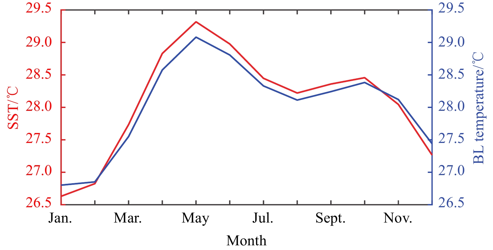
Figure  1.  Seasonal evolution of sea surface temperature (SST, ℃; red line) and temperature averaged within the barrier layer (BL, ℃) (blue line) for the period of 1951–2010, averaged over the Bay of Bengal (5°–25°N, 75°–95°E).

DownLoad: Full-Size Img PowerPoint

Several studies have shown that small sea surface temperature (SST) variability superimposed on the high background SST in the BoB can have a significant effect on ISM activity due to the critical dependence of ISM on deep convection over the BoB and the land-sea temperature contrast (Francis and Gadgil, 2010; Shenoi et al., 2002). Thus, any process that affects SST may play a role in ISM activity. Previous studies mainly focused on the effects of BLs on concurrent SST variability (Balaguru et al., 2012; Breugem et al., 2008; Masson et al., 2005; Qiu et al., 2019; Seo et al., 2009; Wang and Han, 2014; Wang et al., 2011), but the persistent effect of the prior winter (December–February) BL on air-sea interaction in the following seasons and its mechanisms remain unclear. Here we show evidence that an anomalously thick BL in the BoB in the prior winter may advance the ISM onset date and enhance precipitation in June over the South Asian subcontinent. The abnormal BL can impact the evolution of winter SST anomalies through its effects on thermodynamic and dynamic processes. A cloud–SST positive feedback process and penetrative shortwave heating caused by the thinning of the ML associated with the thick BL, act to prolong SST anomalies into the spring (March–May), impacting ISM variability.

The objective of this study is to investigate the contribution of wintertime BL in the BoB to interannual variation of ISM rainfall. The rest of this study is structured as follows: Section 2 introduces the data and methodology. Section 3 discusses the relationships between the prior winter barrier layer thickness (BLT) and Indian summer monsoon activity and the role of the wintertime barrier layer in Section 3. The summary and discussion are provided in Section 4.

2. Data and methods

2.1 Data

The simple ocean data assimilation version 2.2.4 (SODA v2.2.4) dataset, which is available from 1951 to 2010, with a horizontal resolution of 0.5° × 0.5° and 40 vertical levels, is used in this study. The monthly BLT is calculated from monthly SODA temperature and salinity. We have compared the BLT computed from SODA with the observations (World Ocean Atlas, WOA; the research noored array for African-Asian-Australian monsoon analysis and prediction, RAMA; Argo) and other reanalysis product (Ocean Reanalysis System 4, ORAS4). The BLT in SODA generally displays a reasonable seasonal cycle, but it is thinner than in observations (Fig. S1). Regarding the interannual variability of the BoB BLT, there is a very high correlation between SODA and other observations (RAMA and Argo; Figs S2 and S3) as well as the reanalysis dataset (ORAS4; Fig. S4). This indicates that SODA can accurately capture the interannual variability of the BoB BLT, although the amplitude of BLT is weaker than in observations. The atmospheric dataset is from the National Center for Environmental Prediction (NCEP)/National Center for Atmospheric Research (NCAR) Reanalysis 1 (NCEP-1; Kalnay et al., 1996). The atmospheric variables used in this study include precipitation rate, surface wind, surface heat flux, specific humidity, air temperature, and total cloud cover, with a spatial resolution of 2.5° × 2.5° or a T62 Gaussian grid (192 point × 94 point) from 1951 to 2010. In addition, the observed monthly mean rainfall in different regions of India is from the Indian Institute of Tropical Meteorology (IITM) (Parthasarathy et al., 1995). Table S1 provides details on the reanalysis and observational data used in the study. The monthly mean climate indices from 1951 to 2010, including AO, Niño 3.4, and dipole mode index, are downloaded from https://psl.noaa.gov/data/. The fully coupled run output from historical twentieth-century simulation (1850–2005) in the coupled model intercomparison project phase 5 (CMIP5) models is used (Taylor et al., 2012). The simulation uses observed twentieth-century greenhouse gas, ozone, aerosol, and solar forcing. Table S2 lists the 17 CMIP5 models used in the study. Further information on each model is available online at https://esgf-node.llnl.gov/projects/cmip5/. In this study, monthly mean outputs of 55-year historical runs (1951–2005) by CMIP5 models were used, including ocean temperature, salinity, and precipitation.

2.2 Definition of BLT

The BLT is defined as the difference between isothermal layer depth (ILD) and mixed layer depth (MLD). The ILD is defined as the depth at which temperature decreases by 0.2℃ from the reference depth of 10 m (de Boyer Montégut et al., 2007). This avoids the diurnal variability in the top few meters of the ocean (Breugem et al., 2008). The MLD denotes the depth where the density $\Delta\sigma_{{\theta}} $ increases from the reference depth by a threshold following de Boyer Montégut et al. (2007). The variable criterion in density $\sigma_{{\theta}} $ corresponds to a 0.2℃ decrease.

where $ {T_{10}} $ and $ {S_{10}} $ are temperature and salinity at the reference depth of 10 m, and $ {P_0} $ is pressure at sea surface.

2.3 Definition of onset date of summer monsoon

The onset date of the BoB summer monsoon is defined as the first date when the mean meridional gradient of tropospheric temperature between 200–500 hPa over the region of (10°–20°N, 90°–110°E) turns from negative to positive and persists for at least seven consecutive days (Senan et al., 2016; Wang et al., 2009). The onset date of the ISM is defined as the date when the meridional tropospheric temperature gradient changes sign from negative to positive (Goswami and Xavier, 2005; Pradhan et al., 2017). The meridional tropospheric temperature gradient is calculated as the difference in tropospheric temperature (defined as air temperature averaged between 200 hPa and 500 hPa) between a northern box (5°–35°N, 30°–110°E) and a southern box (15°S–5°N, 30°–110°E).

2.4 Diagnostics of mixed layer heat budget

To investigate the processes that control the seasonal evolution of SST, we consider the surface ML heat balance (Foltz and McPhaden, 2009; Lotliker et al., 2016; Thangaprakash et al., 2016) as follows:

where $ {Q_{\mathrm{net}}} $ is the net surface heat flux and it is calculated as

where $ {Q_{\mathrm{shortwave}}} $ is net surface shortwave radiation, $ {Q_{\mathrm{pen}}} $ is shortwave radiation that penetrates below the ML, $ {Q_{{\mathrm{longwave}}}} $ is net longwave radiation, $ {Q_{{\mathrm{latent}}}} $ is latent heat flux, and $ {Q_{{\mathrm{sensible}}}} $ is sensible heat flux. The terms in Eq. (2), from left to right, are ML heat storage rate, $ {Q_{\mathrm{net}}} $, horizontal ML heat advection, vertical entrainment flux, and residual errors (Residual), respectively. Here, $ T $ (℃) is temperature averaged over the ML, $ {T_{-h15}} $ is the temperature 15 m below the ML, $ h $ is the depth of the ML, $ \rho $ is the density of seawater (1024 kg/m³), $ {C_{\mathrm{p}}} $ is the specific heat capacity of seawater [3993 J/(kg·K), $t$ is time (in months), $ u $ ($ v $) is zonal (meridional) velocity (m/s), $ {W_h} $ is vertical velocity (m/s; available directly from the SODA dataset], $ H $ is the Heaviside step function, and x (y) is zonal (meridional) distance. Following Morel and Antoine (1994), the amount of shortwave radiation that penetrates below the ML base is parameterized as

where ${b_1}$ and ${b_2}$ represent the longwave and shortwave extinction coefficient and the factors ${a_1} = 0.6$ and $ {a_2} = 0.4 $, the fractions of total radiation in longwave and shortwave portions of the spectrum, $z$ is positive downward with $ z = 0$ m being the sea surface (Kraus, 1972). Typical values for ${b_1}$ and ${b_2}$ are 0.6 m and 20 m (Paulson and Simpson, 1977; Price et al., 1986; Dewar, 2001).

If we consider the impact of MLD anomalies on the efficiency with which the surface heat flux changes SST, the equation can be written as

In Eq. (5), a bar denotes a monthly climatological mean value, and $ \delta $ represents the difference between an individual month and the monthly climatological mean value. The term $ \delta \left(\dfrac{{{Q_{\mathrm{net}}}}}{{\rho {C_{\mathrm{p}}}h}} \right) $ is decomposed into an anomalous heat flux component $ \left[ \delta \dfrac{{{Q_{\mathrm{net}}}}}{{\rho {C_{\mathrm{p}}}}} \times \right. $$\left. \left({\overline{\dfrac{1}{h}}}\right)\right] $ and an anomalous MLD component $ \left[ \dfrac{{ {{\overline Q_{\mathrm{net}}}} }}{{\rho {C_{\mathrm{p}}}}} \times \delta \left(\dfrac{1}{h} \right) \right] $.

2.5 Model description

The one-dimensional mixed layer model of Price-Weller-Pinkel (PWP; Price et al., 1994) is used in this paper. The model is driven by daily mean heat surface fluxes, precipitation, and 10-m wind components obtained by the NCEP-1. The daily mean surface fluxes are linearly interpolated to the model time step (900 s). The model is initialized with temperature and salinity profiles averaged over the BoB. The ocean variables are obtained from SODA v2.2.4, with a vertical resolution of nearly 10 m from the surface to 80 m, and 10 m to 30 m below. The temperature and salinity profiles are linearly interpolated to the model depth increment (5 m). The penetration of the shortwave scheme used in the model is consistent with the method described in Section 2.4.

2.6 Statistical significance test

Statistical methods of linear correlation and composites are also used in this paper. Both the observations and the reanalysis data mentioned above are detrended before analysis. Statistical significance is tested using a two-tailed Student’s t test (the effective degrees of freedom are recalculated following Roxy (2013) and Sabin et al. (2012) for the composited fields and correlation values, and a Monte Carlo test for the differences in the onset date of the summer monsoon. The confidence levels are described in the figure captions (Figs 3, 7−10, 12, and 13, and Table 1).

3. Results

3.1 Relationships between the prior winter BLT and ISM June rainfall

The BL in the BoB reaches its maximum thickness and horizontal extent during December–February (DJF). Although the BL in the southern BoB is thinner than that of the northern BoB, it is still persistent throughout the winter (Fig. S1c). Thus, we select the BLT regionally averaged over the entire BoB (5°–25°N, 75°–95°E) in DJF for the period of 1951–2010 to study its impact on ISM activity. Since DJF spans two calendar years, hereafter year (0) denotes the reference year, and the following year is labeled with (+1). We analyze the correlations of the DJF BLT averaged over the BoB with each following month’s rainfall over different regions of the South Asian subcontinent during 1951–2010, including total India, central northeast India, northeast India, northwest India, west-central India, and peninsular India (Fig. 2; Kothawale and Rajeevan, 1995). There are significant positive correlations in the total India, west-central India, and central northeast India, with a maximum of up to 0.5 in June at the 95% significance level (Fig. 3a), indicating that an increase (a reduction) in June rainfall over India is connected to a thicker (thinner) BL in the BoB in the prior winter.

Figure  2.  Different regions of India. The map is modified after reference (Kothawale and Rajeevan, 1995).

DownLoad: Full-Size Img PowerPoint

Figure  3.  Pearson’s correlation coefficients between DJF BLT averaged over BoB and subsequent rainfall in total India (white dots), central northeast India (CNE, red dots), northeast India (NE, purple dots), northwest India (NW, yellow dots), peninsular India (cyan dots), and west central India (WC, black dots) (a) and Pearson’s correlation coefficients between DJF BLT and each month’s AO index (black dots), IOD index (white dots), and Niño 3.4 index (cyan dots) in the year (0) and year (+1) (b). The current period is from 1952 to 2010, and the earlier period is from 1951 to 2009. The black lines (chain dotted) denote 95% confidence level.

DownLoad: Full-Size Img PowerPoint

Given that the interannual climate modes such as AO, IOD, and ENSO can trigger anomalies of wind, precipitation, and SST in the tropical Indian Ocean and consequent ISM activity (Ashok et al., 2001; Ashok et al., 2004; Cherchi and Navarra, 2012; Krishnamurthy and Goswami, 2000; Krishnamurthy and Krishnamurthy, 2013; Krishnan and Sugi, 2003), the relationships between the DJF BoB BLT and the following June rainfall might also be driven by these climate modes. To explore this issue, we first calculate the lead-lag correlation coefficients of the DJF BoB BLT and each month’s AO, IOD, and Niño 3.4 indices (Fig. 3b). The DJF BLT variability in the BoB is not associated with the AO, with a quite weak correlation. By contrast, there are obvious negative correlations of the DJF BoB BLT with the previous September–November (SON) IOD index and the simultaneous DJF Niño 3.4 index. This suggests that the interannual variability of winter BLT is modulated by the IOD and ENSO. Hence, we further explore the relationships of the June rainfall of year (+1) with the SON IOD of year (0) and DJF ENSO. The results show that the June rainfall over India is not connected to the previous SON IOD and DJF ENSO, especially after removing the prior winter BL effects (Table 1).

Table  1.  Impact of different factors on June rainfall over India

No.	Region	Variable	Correlation coefficient	Partial correlation coefficient
				Removing IOD (SON)	Removing ENSO (DJF)	Removing BLT (DJF)
1	Total India	IOD	–0.12	–	–0.01	0.05
		ENSO	–0.21	–0.17	–	0.06
		BLT	0.46*	0.45*	0.42*	–
2	Central northeast India	IOD	–0.02	–	0.19	0.14
		ENSO	–0.32*	–0.37*	–	–0.14
		BLT	0.40*	0.42*	0.28*	–
3	Northeast India	IOD	0.05	–	0.12	0.12
		ENSO	–0.09	–0.14	–	0.10
		BLT	0.16	0.19	0.14	–
4	Northwest India	IOD	–0.10	–	–0.11	–0.03
		ENSO	–0.01	0.05	–	0.12
		BLT	0.20	0.18	0.23*	–
5	Peninsular India	IOD	–0.18	–	–0.26	–0.19
		ENSO	0.07	0.21	–	0.08
		BLT	–0.01	–0.08	0.04	–
6	West-central India	IOD	–0.12	–	–0.04	0.05
		ENSO	–0.17	–0.12	–	0.13
		BLT	0.48*	0.47*	0.47*	–
Note: This table shows Pearson’s correlation coefficients and partial correlation coefficients between SON (0) IOD, DJF ENSO indices, and DJF BLT with respect to June (+1) ISM rainfall over different regions of India. The asterisks (*) indicate statistical significance at the 95% level using Student’s t test. The dash (−) indicates no available data.

 | Show Table

DownLoad: CSV

To demonstrate the links between the prior winter BLT and the June rainfall of the following year, here we conduct a partial correlation after removing the influences of IOD/ENSO. Table 1 displays the partial correlations between the DJF BLT and the following June rainfall. The correlation is still statistically remarkable in total India (r = 0.45/0.42), central northeast India (r = 0.42/0.28), and west-central India (r = 0.47/0.47), after excluding the impact of SON (0) IOD/DJF ENSO. Specifically, after removing the influence of DJF ENSO, the evolution of the correlation pattern between the DJF BoB BLT and the following month’s rainfall is the same as before, also with a significant positive correlation in June (Fig. 4b). This is the case after excluding the impact of SON (0) IOD (not shown). All these manifest that prior winter BLT anomalies, although partly forced by the simultaneous ENSO or the previous SON IOD, can potentially contribute to the June rainfall anomalies after removing these climate events. Thus, the prior winter BLT modulated by ENSO/IOD acting as a potential predictor may contribute to the predictability of rainfall in subsequent June over the parts of regions in the South Asian subcontinent. This also implies the potential importance of ocean thermodynamic and dynamic processes associated with prior winter BLT anomalies for regulating SST and atmospheric circulation.

DownLoad: Full-Size Img PowerPoint

3.2 Variations in ISM activity associated with the prior winter BL

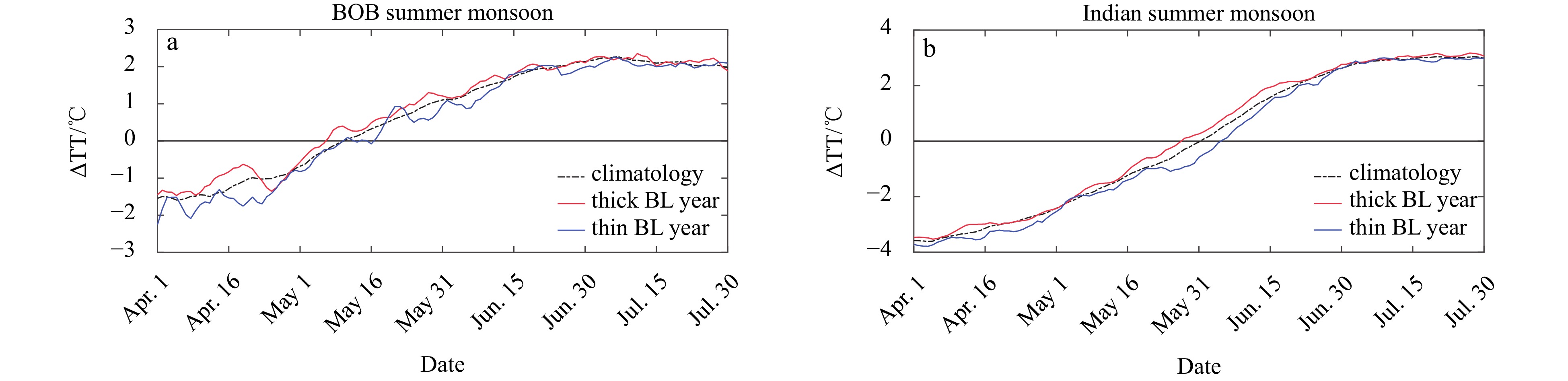
To further understand the effect of the prior winter BL variations in the BoB on ISM activity, we define winter thick and thin BL years based on when the winter BLT anomalies averaged over the entire BoB are greater than one standard deviation or less than minus one standard deviation, respectively. We identify ten thick BL years (1955, 1961, 1970, 1971, 1972, 1976, 1986, 1989, 2001, and 2008) and six thin BL years (1958, 1973, 1991, 1997, 1998, and 2010) according to the criterion above (Fig. 5a). The interannual variation of the wintertime BoB BLT is predominantly controlled by the ILD (Figs 5b and c), with thickness reaching nearly 30 m in thick BL years (red dots on Fig. 5b), but remaining below 20 m for thin BL years (cyan dots on Fig. 5b). The mean onset date of the following the BoB summer monsoon in the thick BL years is 4 d earlier than the climatological mean (May 11), and 10 d earlier than the mean onset date of the thin BL years (Fig. 6a). This difference between the thick/thin BLT years and climatology is significant at the 95% confidence level based on a Monte Carlo test with 10 000 samples. Likewise, it is also true for the Indian summer monsoon: the mean onset date of the subsequent Indian summer monsoon in the thick BL years is also 4 d earlier than the climatological mean (June 1), and 9 d earlier than that of the thin BL years (Fig. 6b), which is also significant at the 95% level. The earlier onset of the ISM indicates that the anomalously thick BL in the prior winter may promote the arrival of the rainy season over the South Asian subcontinent.

Figure  5.  BLT normalized by its mean and standard deviation (a), and BLT (b), ILD (c), and MLD (d) averaged over the BoB (5°–25°N, 75°–95°E) in December–February from 1951 to 2010. When the BLT averaged over December–February is higher (lower) than one standard deviation, it is defined as a thick (thin) BL year. The grey chain dotted lines denote one standard deviation. The red (cyan) dots denote the thick (thin) BL years.

DownLoad: Full-Size Img PowerPoint

Figure  6.  Seasonal evolution of meridional gradient of the daily tropospheric air temperature (℃) in 200–500 hPa over the region of (10°–20°N, 90°–110°E) (a), and meridional difference of the daily tropospheric air temperature (℃) in 200–500 hPa between a northern box (5°–35°N, 30°–110°E) and a southern box (15°S–5°N, 30°–110°E) (b) from April to July, for climatology (black dashed lines), year (+1) of prior winter thick BL years (red lines) and thin BL years (blue lines) (b).

DownLoad: Full-Size Img PowerPoint

Previous studies have demonstrated the influence of SST forcing on ISM rainfall variability (e.g., Chakravorty et al., 2016; Yang et al., 2007), but the role of salinity stratification-induced BL is less clear since there is no direct mechanism for salinity to induce climate patterns. To explain the possible factors that cause the abnormal monsoon onset related to the prior winter BL, we focus on the seasonal evolution of atmospheric and oceanic factors both for prior winter thick and thin BL years. For the prior thick (thin) BL years, a large cooling (warming) in the surface layer occurs over the entire BoB since January (+1) and persists into spring before the onset of ISM (Figs 7b and c). In particular, the SST pattern in March–May (MAM) of the year (+1) bears a resemblance to the composites of SST in this season for the year with the early (late) onset of ISM (Fig. S5). Generally, over the tropical oceans, the tropospheric temperature between 200 hPa and 500 hPa is sensitive to SST forcing. Hence, in the thick BL years, a dramatically strengthened tropospheric temperature gradient between land and sea which acts as an effective index of the onset of ISM is observed in the monsoon region (Fig. 8b), physically consistent with the seasonal evolution of SST anomalies in the BoB (Fig. 8a). As a result, it results in a large-scale atmospheric response pattern: the southwesterly winds significantly strengthen over the BoB in May of the year (+1) and extend further northward (Fig. 9b), leading to more moisture transported from the tropical Indian Ocean to the South Asian subcontinent at a low level, the intensified moisture convergence (Fig. 8c) and further the peak rainfall in June of the year (+1) (Fig. 9b). The intensified moisture convergence over India in June is significantly correlated with the prior winter BLT (Fig. 8e) and June rainfall over India (Fig. 8f). The opposite is true for the prior winter thin BL years (Figs 8d and 9c).

DownLoad: Full-Size Img PowerPoint

Figure  8.  Seasonal evolution of SST (℃) averaged over BoB (a) and land-sea thermal contrast in the tropospheric (200–500 hPa average) temperature (b) from January to December, for climatology (black solid lines), year (+1) of prior winter thick BL years (red lines) and thin BL years (blue lines); and composite of moisture flux [kg/(m·s)] anomalies averaged over April (+1)–June (+1) for prior winter thick BL years (c) and thin BL years (d); and scatterplots between June (+1) moisture flux convergence [×10⁵ kg/(m²·s)] averaged over India (10°–30°N, 70°–90°E) and DJF BLT (m) averaged over the BoB (e) and June (+1) precipitation (mm) averaged over India (f). In a and b, the land-sea thermal contrast in the troposphere (200–500 hPa) is estimated as the difference in the values between the boxes over the South Tibetan Plateau (25°–40°N, 65°–95°E) and the BoB (5°–25°N, 75°–95°E). The definition of land-sea thermal contrast follows Li and Xiao (2021). The black chain dotted line denotes the temperature of 28℃. The triangles denote statistical significance at the 90% confidence level by two-tailed Student’s t test. In b and c, the red arrows denote statistical significance at the 90% confidence level by two–tailed Student’s t test. In e and f, the gray lines indicate the least-squared fits and the correlation coefficients (r) are statistically significant at the 95% confidence level.

DownLoad: Full-Size Img PowerPoint

DownLoad: Full-Size Img PowerPoint

3.3 Role of wintertime salinity BL

3.3.1   Evolution of surface heat flux

From the above results, the spatial pattern of SST anomalies linked to the prior winter BoB BLT anomalies results in atmospheric circulation response. Hence, we pose a critical question: what is the cause of prior winter SST anomalies and their persistence into the pre-ISM season? We compute ML heat budget to examine the contributions of individual components in surface heat forcing to SST anomalies. For the prior winter thick BL years, cold SST anomalies appear in October–November of the year (0) (Fig. 10g), which is attributed to the intensified latent heat loss (Figs 10f and 11e) due to the enhanced surface winds (Fig. 10j). Furthermore, the increased cloudiness (Fig. 10i) over the BoB leads to a decrease in shortwave radiation flux absorbed by the ML during October (0)–January (+1) (Figs 10b and 11b), which prolongs the cold SST anomalies for several months (Fig. 10g). Tanimoto and Xie (2002) suggested positive feedback between SST and low-level coluds over the tropical oceans, namely when SST cools, cloud amount increases, leading to less shortwave radiation absorbed by the sea surface and further cooling of the ocean. Therefore, the cold SST anomalies in year (0) induced by the increased surface latent heat flux could persist into year (+1), through the positive cloud-SST positive feedback.

Figure  10.  Anomalous evolution of net heat flux (a), net shortwave radiation flux (b), penetrative shortwave radiation flux (c), longwave radiation flux (d), sensible heat flux (e), latent heat flux (f), SST (g), mixed layer depth (MLD, h), total cloud cover (TCDC, i), and wind speed (j), averaged over the BoB from September (0) to September (+1), for prior winter thick BL years (blue bars) and thin BL years (red bars). Note that Y-axis ranges in a–f are inconsistent. The red asterisks (*) denote statistical significance at the 90% confidence level by two-tailed Student’s t test.

DownLoad: Full-Size Img PowerPoint

3.3.2   Evolution of subsurface temperature

Over the tropical oceans, the deep convection remains weak and is rarely observed for SST < 26.5℃, while the monotonic increase in precipitation with respect to SST is limited to a range of 26.5–29.0℃, with sharp decay with further increase in SST (Gadgil et al., 1984; Graham and Barnett, 1987; Roxy, 2013; Sabin et al., 2012; Waliser et al., 1993; Zhang, 1993). Thereby, if the sea surface cools excessively in thick BL years, it would weaken or even disrupt deep atmospheric convection over the BoB. In this subsection, we will investigate the potential role of thick BLs in modulating the BoB SST anomalies.

As stated in the introduction, shallow haline stratification and thick BL could lead to temperature inversions in winter in the BoB (Fig. 1), that is, cool surface water overlaying warm subsurface water. In the thick BL years, thicker BoB BL would be expected to intensify the temperature inversions and lead to significantly strengthened subsurface warming relative to the climatology (Fig. 12a), particularly during DJF (+1). Note that there is no temperature inversion in the BoB during the MAM (Fig. 1), but we also find a subsurface warming anomaly at this season (Fig. 12a). This is attributed to the increased shortwave penetration (Fig. 10c) induced by the shallower ML (Fig. 10h). The anomalous subsurface warming tends to restrict cold SST anomalies caused by atmospheric forcing through the vertical entrainment, which favors the sufficient near-surface humidity and the development of deep convection over the BoB before the ISM onset.

To further confirm the role of the winter BLs, we examine the ML heat budget using Eq. (2). Although surface net heat flux is a significant contributor to the ML heat budget in the BoB (Fig. 11a), vertical processes cannot be neglected (Fig. 13b), in particular during winter. Note that the contribution of vertical entrainment may be underestimated since it is difficult to separate the vertical entrainment term from the residual term. Figure 13b displays that vertical entrainment induces anomalous warming (cooling) tendencies in the BoB for thick (thin) BL years, illustrating that the variability of vertical entrainment is associated with prior winter thick (thin) BL. From September (0) to March (+1), the anomalies in vertical entrainment vary nearly in phase with the BLT anomalies, with a maximum in winter (Figs 13b and d). Yet, this coherence of abnormal evolution between vertical entrainment and BLT starts to diminish from April (+1) due to the weakening of the BL effect. In general, vertical entrainment scales with the temperature difference between the base and the core of the ML (i.e., $ \Delta T = {T_{ - h}} - \overline {T\;} $; Kraus and Turner 1967; Stevenson and Niiler 1983). Therefore, we also estimate the evolution of temperature difference averaged over the BoB in order to further confirm the potential effect of BL on the surface temperature by vertical processes. As we expected, positive (negative) anomalies in temperature difference appear in September (0) and persist into March (+1) for thick (thin) BL years (Fig. 13c), which is consistent with the evolutions in vertical entrainment (Fig. 13b) and BLT (Fig. 13d). It implies that the subsurface anomalous warming throughout the winter and even into March (+1) induced by the prior winter thicker BLs is entrained into the ML, acting as damping for cold SST anomalies caused by atmospheric forcing and hence favoring the development of deep convection in the following season.

Figure  11.  Seasonal evolution of anomalous SST tendency induced by surface heat flux and ML. Anomalous evolution of net surface heat flux term (a, f), net shortwave radiation flux term (b, g), longwave radiation flux term (c, h), sensible heat flux term (d, i), and latent heat flux term (e, j) in Eq. (5) averaged over the BoB from September (0) to September (+1), for prior winter thick BL years (the first column) and thin BL years (the second column). The blue bars denote the anomalous surface heat flux component $\delta \dfrac{{{Q_{\mathrm{net}}}}}{{\rho {C_{\mathrm{p}}}}} \times \left(\overline {\dfrac{1}{h}}\right)$, and the red bars denote the anomalous MLD component $ \dfrac{{ {{\overline Q_{\mathrm{net}}}} }}{{\rho {C_{\mathrm{p}}}}} \times \delta \dfrac{1}{h} $. The red lines denote the sum of the anomalous surface heat flux component and anomalous MLD component. The blue lines denote the anomalies simultaneously considering surface heat flux and MLD.

DownLoad: Full-Size Img PowerPoint

Figure  12.  Anomalous evolution of temperature averaged over BoB from January (0) to December (+1), for prior winter thick BL years (a) and thin BL years (b). The black lines denote the zero contour. The black spots denote statistical significance at the 90% confidence level by two-tailed Student’s t test.

DownLoad: Full-Size Img PowerPoint

Figure  13.  Anomalous evolution of penetrative shortwave radiation (a), vertical entrainment (b), ${T_{ - h}} - \overline {T\;} $ (℃; the temperature at the base of mixed layer minus the temperature of mixed layer average) (c), and BLT (d), averaged over the BoB from September (0) to September (+1), for prior winter thick BL years (blue bars) and thin BL years (red bars). The red asterisks (*) denote statistical significance at the 90% confidence level by two-tailed Student’s t test.

DownLoad: Full-Size Img PowerPoint

3.3.3   Links of shallow ML to prior winter thick BL

In the above discussion, we note that a thicker DJF BL is accompanied by a shallower MAM (+1) ML in the BoB, as illustrated in Fig. 10h. It indicates that the variability in MAM (+1) MLD is related to the prior winter BLT. Figure 14a demonstrates that this is the case, by identifying a significant correlation between the MAM (+1) MLD and DJF BLT averaged over the BoB (r = –0.25, p < 0.1). In the following, we will examine the mechanism that links MAM (+1) MLD to the prior winter BLT. Figures 14b and c display the pronounced relationships between the MAM (+1) precipitation and the simultaneous MLD (r = –0.37, p < 0.05) and DJF BLT (r = 0.24, p < 0.1) averaged over the BoB, indicating that the prior winter thick BL in the BoB induces the rainfall increase during MAM season and the associated shoaling of ML. The shallower ML allows more shortwave radiation to penetrate below the ML, which leads to surface cooling through a decrease in the surface net heat flux (e.g., Tian and Zhang, 2023). As shown in Fig. 10, there is an obvious increase in shortwave penetration during MAM (+1) for thick BL years (Fig. 10c), which is associated with the shallow ML anomalies (Fig. 10h). This increased shortwave penetration contributes to cooler-than-normal SST during MAM (+1) (Fig. 10g). Over the tropical oceans, the change of averaged tropospheric temperature is approximately linear with the SST variability (Su et al., 2003; Zeng et al., 2016). As a result, the resultant SST cooling causes a pronounced increase in meridional land-sea thermal contrast in the troposphere during May (+1) and June (+1), resulting in the enhanced rainfall over India in June (+1) through the modulation of atmospheric circulation, in agreement with the results in Section 3.2.

Figure  14.  Scatterplots between DJF BLT and MAM (+1) MLD (a), and between MAM (+1) precipitation rate and MAM (+1) MLD (b) and DJF BLT (c), averaged over BoB. The gray lines indicate the least-squared fits.

DownLoad: Full-Size Img PowerPoint

3.3.4   Model validation

The one-dimensional mixed layer model of PWP is further used to investigate the influence of the prior winter BL on entrainment flux. In the model, three stability criteria (static instability, bulk, and gradient Richardson number) are involved in the turbulent mixing process. Two experiments are conducted to evaluate the effect of the prior winter BL on the evolution of mixed layer temperature. In the two experiments, the model is initialized with the composites of temperature and salinity profiles averaged over the BoB from December (0) to February (+1) for prior winter thick (thin) BL years, driven by the composites of atmospheric forcing for the selected thick (thin) BL years. The only difference between the two experiments is the initial salinity stratification in the upper ocean: one has salinity stratification within the isothermal layer, which denotes the presence of a BL; in the other, salinity is homogenous in the isothermal layer, representative of removing the BL (Experiment Rm-BL; Figs 15a and b). For the BL scheme, the averaged temperature of the ML from January (+1) to March (+1) in the thick (thin) BL years is higher by up to about 0.1℃ (about 0.2℃) than that of the Rm-BL scheme (Fig. 15c), which supports the results based on a diagnostic method (Fig. 13b). The simulated averaged temperature of the ML increases more in the BL case for thin BL years, which is attributed to the reduced heat capacity of a thinner ML (Fig. 15d). Moreover, note that the higher averaged temperature of the ML in the BL case for both thick and thin years gradually reduces starting in late March (+1) in accordance with the seasonal evolution of MLD, indicating that the impact of salinity stratification on vertical mixing and vertical exchanges of heat gradually weakens. Previous studies have shown that a slight change in sea surface temperature is important for inducing a change in atmospheric circulation in the tropical oceans (Deser et al., 2010; Liao and Wang, 2021; Trenberth et al., 1998), due to the sensitivity of the tropical atmosphere response to sea surface temperature variation (Bjerknes, 1969). The simulation results using the PWP model further confirm that the prior winter BL can reduce the entrainment of cold thermocline water, favoring subsurface warming to limit the excessive sea surface cooling induced by atmospheric forcing in the thick BL years.

Figure  15.  Initial fields in the experiments are the composited temperature (a) and salinity (b) profiles averaged over BoB (5°–25°N, 75°–95°E) from December (0) to February (+1), for the selected prior winter thick (thin) BL years, and the evolution of averaged temperature of the ML (c) and MLD (d) simulated by the Price-Weller-Pinkel mixed layer model. For a and b, the model is driven by the composited atmospheric forcings averaged over the BoB, for prior winter thick (thin) BL years. The solid (dot) black and solid (dot) red lines represent the BL and removed BL (Rm-BL) conditions.

DownLoad: Full-Size Img PowerPoint

In summary, the prior winter thick BLs serve as a dynamical thermostat by restraining cold thermocline water entrainment into the ML: a thicker BL damps the surface flux-induced SST cooling during JFM (+1) (due to entrainment) and sustains the existing cooling during MAM (+1) (due to penetrative shortwave radiation). The damping effect of thick BLs serves to restrict excessive cooling of the sea surface during JFM (+1) and thus aids in developing the deep convection, leading to more precipitation over the BoB in the MAM (+1) season for the thick BL years. This enhanced precipitation leads to strong salinity stratification and shallower MLD in the BoB, allowing more penetrative shortwave radiation during MAM (+1), which further maintains the existing sea surface cooling in the BoB and intensifies the southwesterly winds through an increase in the tropospheric temperature gradient between land and sea. The intensified southwesterly winds allow more moisture transported from the tropical Indian Ocean to the South Asian subcontinent at a low level and result in the increased ISM rainfall in June (+1) along with the northward migration of the major rain band from the eastern tropical Indian Ocean to the South Asian subcontinent.

4. Summary and discussion

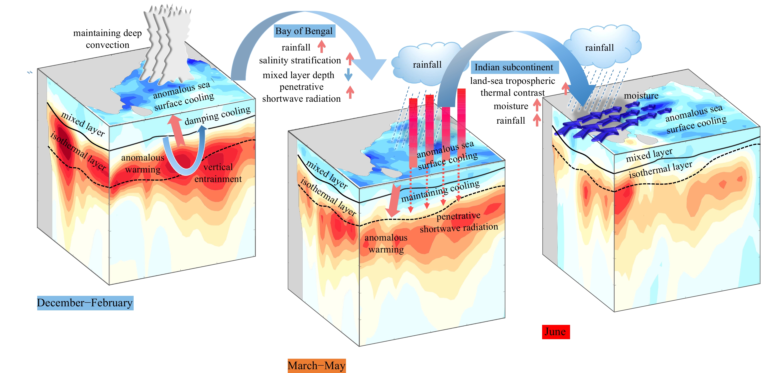
The purpose of the study is to clarify the persistent impact of regional winter BLs in the BoB on the ocean-atmosphere interactions and regional rainfall over the South Asian subcontinent. Our findings test the hypothesis that prior winter salinity BL in the BoB is significantly connected to rainfall in June over the South Asian subcontinent. The prior winter BL anomalies in the BoB can modulate abnormal ISM activity by modifying the monsoon-related atmospheric circulation and oceanic dynamic process in the tropical Indian Ocean. A schematic of the mechanisms is shown in Fig. 16. For the prior winter thicker-than-normal BL years, the SST cooling is caused by intensified latent heat loss starting in October of the year (0), which is maintained by the wind-evaporation feedback. Additionally, the surface layer absorbs less shortwave radiation owing to increased cloud cover, which can also prolong sea surface cooling into the subsequent year through positive low-level cloud-SST feedback. However, if the sea surface excessively cools, the deep convection over the BoB will be weak and even interrupt. The warmer subsurface water associated with the prior winter thick BL is entrained into the ML during JFM (+1), which tends to damp the excessive sea surface cooling induced by atmospheric forcing (wind-induced latent heat loss and solar radiation reduction) and favor more near-surface humidity and the development of deep convection in MAM (+1) season (Fig. S6). Thus, the increased precipitation over the BoB occurs in the MAM (+1) season along with the northward migration of the major rain band from the eastern tropical Indian Ocean to the BoB. This enhanced precipitation weakens ocean salinity and MLD, allowing more penetrative shortwave radiation during MAM of the year (+1), which further maintains the existing sea surface cooling and therefore leads to an increased meridional land-sea thermal contrast in the troposphere. As tropospheric temperature is related to the deep heat source, it makes good sense to use the change of sign of the tropospheric temperature gradient for defining onset as well as “withdrawal” of monsoon as it relates to winds turning southwesterly near the surface as well as above the boundary layer (Chou, 2003; Goswami and Chakravorty, 2017; Kamae et al., 2014; Sutton et al., 2007; Webster et al., 1998; Wu et al., 2012). Thus, the meridional gradient of tropospheric temperature can be responsible for the deep summer monsoon circulation (Webster et al., 1998). At that point, there is possibly a large-scale atmospheric adjustment: the ISM onset is earlier than normal along with the enhanced southwesterly winds, and the ISM precipitation over India is enhanced. The results from this study suggest that the winter thick BL acts as a dynamical thermostat by restraining cold thermocline water entrainment into the ML.

Figure  16.  Schematic of the mechanisms of the prior winter’s anomalously thick BL modulating the June rainfall over India. The meridional section is the average temperature anomalies from 75°E to 95°E over the BoB. The zonal section is the average temperature anomalies from 5°N to 25°N over the BoB. The horizontal section is the sea surface temperature anomalies in the BoB. The solid (dashed) black lines indicate MLD (ILD). The little pink (light blue) arrows indicate an increase (decrease) of the atmospheric and oceanic factors. In December–February, the vertical entrainment of the subsurface warm water associated with prior winter thick BL anomalies damps the sea surface cooling to maintain the deep atmospheric convection. In March–May, sufficient near-surface humidity increases rainfall, enhancing salinity stratification and reducing MLD. More shortwave radiation penetrates the ML, maintaining surface cooling and increasing the land-sea thermal gradient. In June, more moisture is transported into the South Asian subcontinent, which therefore results in the increase of rainfall over India.

DownLoad: Full-Size Img PowerPoint

Note that there is a basin-wide cooling/warming (Fig. 7) and intensified/reduced southwesterly winds (Fig. 9) over the entire tropical Indian Ocean in the prior winter thick/thin BL years, which resembles the Indian Ocean basin mode and atmospheric response pattern regulated by ENSO. However, SST variability in the BoB is significantly correlated with the BoB DJF BLT after excluding the impact of ENSO, with a correlation coefficient of –0.25 (p < 0.1; not shown), particularly in the MAM (+1) season. This suggests that although the basin-wide SST anomalies in winter are modulated by the climate modes, the BoB SST anomalies during the following spring are also associated with the BoB BLT in the prior winter. In this study, we mainly emphasize that the BoB winter salinity BL acting as a dynamic thermostat by restraining cold thermocline water entrainment into the ML modulates the regional ocean-atmosphere interactions and the subsequent rainfall over the South Asian subcontinent by adjusting the thermodynamic and dynamic process in the upper ocean. Our study has an important implication that the winter thick BL in the BoB may have the power to serve as a great predictor of enhanced rainfall in June over the South Asian subcontinent.

It is natural to ask whether current state-of-the-art coupled models participating in CMIP5 can reproduce the observed relationship between the prior winter BLT and June ISM rainfall. We analyze the 55-year (1951–2005) outputs of historical runs by 17 coupled models. Only three (BCC-CSM1-1, GFDL-CM3, and GFDL-ESM2M) out of 17 models can simulate the positive relationship between prior winter BLT and June ISM rainfall averaged over the South Asian subcontinent, but the correlation coefficients are relatively low (Fig. S7). In contrast, other models fail to simulate the observed relationship between prior winter BLT and June ISM rainfall. The ensemble means of 17 CMIP5 models show negligible impacts of the prior winter BL on the ISM rainfall because most coupled models in CMIP5 still have difficulties in realistically simulating interannual variations of salinity BL and ISM rainfall. To some extent, most of the models, except CNRM-CM5, GISS-E2-H, and MRI-CGCM3, simulate anomalously thin BLs averaged over December–February (Fig. S8). In addition, all models except CCSM4, MIRO-ESM, and MIRO-ESM-CHEM show large negative biases in June ISM rainfall over and around India (Fig. S9). This suggests that the weak BL in CMIP5 models, combined with other factors, may be partially responsible for the ISM precipitation biases.

Our study further indicates that there is a clear need to evaluate the performance of climate models in reproducing the observed BLs in the BoB. Assessing the climate biases caused by the salinity BL effects in coupled climate models provides a step toward improving air-sea coupled model performance. These kinds of studies will greatly improve our understanding of the effect of the salinity BL on large-scale climate variations, including the ISM.