Feng Nan, Zhuolin Li, Jie Yu, Suixiang Shi, Xinrong Wu, Lingyu Xu. Prediction of three-dimensional ocean temperature in the South China Sea based on time series gridded data and a dynamic spatiotemporal graph neural network[J]. Acta Oceanologica Sinica, 2024, 43(7): 26-39. doi: 10.1007/s13131-023-2252-0
Citation:
Feng Nan, Zhuolin Li, Jie Yu, Suixiang Shi, Xinrong Wu, Lingyu Xu. Prediction of three-dimensional ocean temperature in the South China Sea based on time series gridded data and a dynamic spatiotemporal graph neural network[J]. Acta Oceanologica Sinica, 2024, 43(7): 26-39. doi: 10.1007/s13131-023-2252-0
Feng Nan, Zhuolin Li, Jie Yu, Suixiang Shi, Xinrong Wu, Lingyu Xu. Prediction of three-dimensional ocean temperature in the South China Sea based on time series gridded data and a dynamic spatiotemporal graph neural network[J]. Acta Oceanologica Sinica, 2024, 43(7): 26-39. doi: 10.1007/s13131-023-2252-0
Citation:
Feng Nan, Zhuolin Li, Jie Yu, Suixiang Shi, Xinrong Wu, Lingyu Xu. Prediction of three-dimensional ocean temperature in the South China Sea based on time series gridded data and a dynamic spatiotemporal graph neural network[J]. Acta Oceanologica Sinica, 2024, 43(7): 26-39. doi: 10.1007/s13131-023-2252-0
Prediction of three-dimensional ocean temperature in the South China Sea based on time series gridded data and a dynamic spatiotemporal graph neural network
Ocean temperature is an important physical variable in marine ecosystems, and ocean temperature prediction is an important research objective in ocean-related fields. Currently, one of the commonly used methods for ocean temperature prediction is based on data-driven, but research on this method is mostly limited to the sea surface, with few studies on the prediction of internal ocean temperature. Existing graph neural network-based methods usually use predefined graphs or learned static graphs, which cannot capture the dynamic associations among data. In this study, we propose a novel dynamic spatiotemporal graph neural network (DSTGN) to predict three-dimensional ocean temperature (3D-OT), which combines static graph learning and dynamic graph learning to automatically mine two unknown dependencies between sequences based on the original 3D-OT data without prior knowledge. Temporal and spatial dependencies in the time series were then captured using temporal and graph convolutions. We also integrated dynamic graph learning, static graph learning, graph convolution, and temporal convolution into an end-to-end framework for 3D-OT prediction using time-series grid data. In this study, we conducted prediction experiments using high-resolution 3D-OT from the Copernicus global ocean physical reanalysis, with data covering the vertical variation of temperature from the sea surface to 1 000 m below the sea surface. We compared five mainstream models that are commonly used for ocean temperature prediction, and the results showed that the method achieved the best prediction results at all prediction scales.
On 21 April 2021 local time (20 April UTC), the Indonesian Navy submarine (KRI Nanggala-402) sank near the Lombok Strait, ~100 km north of the Bali Island (see magenta star in Fig. 1a), with 53 crew members dead. On the basis of Moderate Resolution Imaging Spectroradiometer (MODIS) satellite images (Jackson, 2007), NASA demonstrated that powerful “underwater waves” happened in the treacherous region and likely hit the vessel resulting in its disappearance (https://www.npr.org/2021/04/30/992496772/). Besides, NASA reported that the collapse depth of submarine KRI Nanggala-402 was ~200 m, but official reports on the local underwater waves and the voyage depth of the submarine were still lacking. This phenomenon was referred to as oceanic internal solitary waves (hereinafter ISWs). An important behaviour of ISWs is causing large vertical displacements and downward currents in a short time in the ocean interior, and therefore may drag the submarine down to the collapse depth (i.e., ~200 m), where the water pressure exceeds the endurance limit of the submarine.
Figure
1.
Bathymetry around the Indonesia including the Lombok Strait (a), the submarine wreckage location is marked as a magenta star; a satellite image on 25 April 2005 derived from the MODIS (b), in which blue arrows represent wave propagation directions; and numerically-predicted sea surface height gradients ($ \left|\nabla \eta \right| $) at 01:00 UTC on 20 April 2021 (c).
There are three conditions generating oceanic ISWs, namely the oscillatory surface (i.e., barotropic) tides, the abrupt topography (e.g., underwater sill and slope), and the stratified water. The Lombok Strait was well-known for all three (Murray and Arief, 1988; Mitnik et al., 2000; Ningsih et al., 2010; Purwandana et al., 2021), so whether the ISWs were the culprit causing the shipwreck in the Lombok Strait was of particular interest. To address this problem, we need to understand the physical dynamics and spatial characteristics of ISWs. Here two approaches were used to investigate ISWs in the Lombok Strait: first using the satellite image to present the spatial variability of ISWs, second numerically reproducing the ISW dynamics on the day of the accident.
Convergence/divergence of the currents induced by ISWs on the ocean surface contributed to strong modulations of sea surface roughness, thereby resulting in distinctive features in the optical true-color images (e.g., Susanto et al., 2005). A snapshot on 25 April 2005 (Fig. 1b) depicted that the Lombok Strait generated ISWs radiated both northward and southward. Three stages of northward-going ISWs were captured in the satellite image (Fig. 1b), namely the generation, propagation and shoaling processes. The ISW was presented as an isolated wave with a short crest length on the stage 1, but converted to a wave packet with a long crest length on the stage 2. Eventually on the stage 3, the wave packet approached the wreckage site and reached the shallow region near the Kangean Island (Fig. 1b).
Based on ~7 000 MODIS images over the past 20 years from 2002 to 2021, we identified wave occurrences in April and estimated wave amplitudes by a theoretical method (KdV theory, Ostrovsky and Stepanyants, 1989).
where the parameters $ {c}_{0} $, $ \alpha $ and $\, \beta $ are linear long-wave phase speed, nonlinear coefficient and dispersion coefficient, respectively. $ \alpha $ and $\, \beta $ are coefficients associated with background continuous stratification and water depth. Here we calculated spatio-temporal varying $ \alpha $ and $ \,\beta $ using monthly climatological density profiles from the WOA18 dataset (World Ocean Atlas 2018) with a horizontal grid resolution of 0.25°. Amplitudes of the ISWs can be extracted in the satellite images (Zheng et al., 2001), following the equation:
where $ D $ is the distance between the center of the bright and dark stripes within the leading wave in the MODIS true-color images, $ l $ is the characteristic half width of an ISW, and $ {\eta }_{0} $ is the estimated wave amplitude.
Regardless of northward- or southward-going ISWs, ISWs were commonly appearing in April (i.e., the month of submarine sinking event), which provided the evidences that ISWs could be the culprit to the shipwreck in April 2021. In terms of northward-going ISWs, the KdV theory was applied to extract wave amplitudes on different stages (Fig. 1a) based on the distance between the bright and dark stripes in the MODIS images. Overall, ISWs had the largest amplitude of ~70 m shortly after generating over the sill (Stage 1), then decreased from ~50 m in the deep water (Stage 2) to ~35 m at the wreckage site (Stage 3).
In comparison with satellite observations, numerical simulations are a more effective approach to characterize the ISW structures in the ocean interior and reproduce wave dynamics in the Lombok Strait (Aiki et al., 2011). Hence, we implemented a three-dimensional primitive equation ocean solver (MIT general circulation model, MITgcm) in the nonhydrostatic mode with realistic conditions during a spring tidal period from 00:00 UTC 17 April 2021 to 00:00 UTC 22 April 2021. Cable News Network (CNN) reported that the submarine started diving at 03:00 on 21 April local time (20:00 UTC 20 April) but lost contact at 04:25 on 21 April local time (21:25 UTC 20 April), so we mainly focused on 20 April (UTC) 2021 (Fig. 2). Model configurations were presented as follows.
Figure
2.
Numerically-predicted sea surface height gradients ($ \left|\nabla \eta \right| $) (a) and numerically-predicted isotherms ($ T $) from 28.5°C to 9°C (bending line in b, d and f from top to bottom) with a interval of 1.5°C and wave-induced velocity ($ {U}_{\rm {bc}} $, color shade) along the transect (red dashed line in panel a) (b) at 05:30 UTC on 20 April 2021; c and d are the same as a and b but at 13:30 UTC on 20 April 2021, and e and f are at 21:30 UTC on 20 April 2021. The wreckage site is marked as the magenta star and ISWs on three stages are marked in blue boxes. z represents water depth.
Model bathymetry data was derived from the ETOPO1 global dataset (Amante and Eakins, 2009). To ensure these waves were physically derived rather than products of numerical dispersion (Vitousek and Fringer, 2011), a resolution condition ($ \Delta x<{h}_{\rm p} $) needs to be satisfied, where $ {h}_{\rm p} $ was defined as the depth of the internal interface (pycnocline depth). According to the WOA18 climatology dataset of stratification, $ {h}_{\rm p} $ was approximately equal to 100 m in April, we therefore set horizontal cell ($ \Delta x $) as 100 m in both the longitudinal and latitudinal directions. The entire model domain consisted of 3 000$ \times $2 000 grid cells with 60 vertical layers ranging from 10 m from the surface to 100 m near the sea bed. The initial model stratification was obtained from the climatology dataset WOA18 by spatially averaging the monthly output in April, resulting in horizontally homogeneous temperature initial conditions.Salinity was set as a constant value of 34.5. The model was driven by eight main tidal constituents (M2, S2, N2, K2, K1, O1, P1, Q1) on the boundaries with values derived from the Oregon State University TOPEX/Poseidon Solution (TPXO8-atlas data) with (1/30)° resolution. A 10 km wide sponge layer was imposed on each lateral boundary to absorb internal waves and avoid reflection back to the inner region. We started a 5-d simulation from 17 April (UTC) 2021. Quasi-steady conditions occurred after 3 d, so the model results were analyzed over the remaining 2 d (20–21 April). More details of model configurations were shown in Table 1.
Analogous to the stripe brightness in the satellite images, numerically-predicted surface height gradients can measure the surface roughness induced by ISWs. A model snapshot was selected at 01:00 UTC on 20 April (Fig. 1c). Three stages of northward-going ISWs were clearly identified, as well as a southward-going ISW packet, whose locations were reasonably consistent with those in the satellite image (Fig. 1b). To a certain extent, it verified the model accuracy. Moreover, a transect (red dashed line in Fig. 1c) along the wave propagation directions was selected to demonstrate the vertical structures of ISWs from generation in the Lombok Strait to the shoaling process at the wreckage site (Figs 2 and 3).
Figure
3.
Numerically-predicted sea surface height gradients ($ \left|\nabla \eta \right| $) (a) and numerically-predicted isotherms ($ T $) from 28.5°C to 9°C (bending line in b, d and f from top to bottom) with a interval of 1.5°C and wave-induced velocity ($ {U}_{\rm {bc}} $, color shade) along the transect (red dashed line in panel a) (b) during the period from 19:30 UTC 20 April to 22:30 UTC 20 April with the time interval of 1.5 h. It characterizes the ISW properties right before and after it passing the wreckage site. The wreckage site is marked as the magenta star. z represents water depth.
The model results demonstrated that ISWs, generated from the Lombok Strait, presented different characteristics on three stages, i.e., with the amplitude of 90 m, 50 m and 40 m on the generation, propagation and shoaling processes (Figs 2b, d and f). Maximum ISW amplitudes mainly occurred at the water depth between 150 m to 400 m, covering the submarine’s collapse depth of ~200 m, thereby dragging it down to a more dangerous depth. At 21:30 UTC on 20 April 2021, an ISW packet with a leading wave amplitude of 40 m was shoaling and passing the shipwreck site (Fig. 2f). This time is in coincidence with the reported missing time. The ISW packet had a long characteristic width of approximately 50 km and remained fluctuations for over 10 h. Even though the following waves have relatively small amplitudes of 10−30 m, the continuous wave motions are likely to have a sustained impact on the submarine (Fig. 3). It is noteworthy that the future submarine motion should be more careful when passing the Lombok Strait (Stage 1), where the local ISWs might have a reasonably large amplitude of 90 m (Fig. 2b) in the ocean interior. In future, when submarines sail across the Lombok Strait, the voyage depths would be better in the upper 150 m, where the ISW amplitudes are relatively small, so the ISW is unable to drag the vessel down to a dangerous depth.
In summary, intense ISW events in the Lombok Strait have remarkable vertical displacements within a few minutes, thereby significantly affecting the underwater navigation and action of submarine. This numerical study concludes an ISW packet with a maximum amplitude of 40 m at the wreckage site on 20 April (UTC) 2021, which is likely the culprit to the sunk KRI Nanggala-402 submarine. Although satellite observations and numerical modelling have illustrated the crucial role of ISWs in the ocean interior, in situ observations of ISWs are needed to tell a more complete story in the future.
Acknowledgements
We acknowledge the use of MODIS-Aqua imagery from the NASA Worldview application (https://worldview.earthdata.nasa.gov). The numerical simulation is supported by the High Performance Computing Division and HPC managers of Wei Zhou and Dandan Sui in the South China Sea Institute of Oceanology.
Aparna S G, D’souza S, Arjun N B. 2018. Prediction of daily sea surface temperature using artificial neural networks. International Journal of Remote Sensing, 39(12): 4214–4231, doi: 10.1080/01431161.2018.1454623
Barnston A G, Tippett M K, Ranganathan M, et al. 2019. Deterministic skill of ENSO predictions from the North American Multimodel Ensemble. Climate Dynamics, 53(12): 7215–7234, doi: 10.1007/s00382-017-3603-3
Collins D C, Reason C J C, Tangang F. 2004. Predictability of Indian Ocean sea surface temperature using canonical correlation analysis. Climate Dynamics, 22(5): 481–497, doi: 10.1007/s00382-004-0390-4
Dong Yihe, Cordonnier J B, Loukas A. 2021. Attention is not all you need: Pure attention loses rank doubly exponentially with depth. In: Proceedings of the 38th International Conference on Machine Learning. PMLR, 2793–2803
Gao Ziheng, Li Zhuolin, Yu Jie, et al. 2023. Global spatiotemporal graph attention network for sea surface temperature prediction. IEEE Geoscience and Remote Sensing Letters, 20: 1500905
Garcia-Gorriz E, Garcia-Sanchez J. 2007. Prediction of sea surface temperatures in the western Mediterranean Sea by neural networks using satellite observations. Geophysical Research Letters, 34(11): L11603
Glorot X, Bordes A, Bengio Y. 2011. Deep sparse rectifier neural networks. In: Proceedings of the 14th International Conference on Artificial Intelligence and Statistics. Fort Lauderdale, 315–323
Guo Shengnan, Lin Youfang, Feng Ning, et al. 2019. Attention based spatial-temporal graph convolutional networks for traffic flow forecasting. In: Proceedings of the Thirty-Third AAAI Conference on Artificial Intelligence and Thirty-First Innovative Applications of Artificial Intelligence Conference and Ninth AAAI Symposium on Educational Advances in Artificial Intelligence. Honolulu: AAAI Press, 922–929
He Kaiming, Zhang Xiangyu, Ren Shaoqing, et al. 2016. Deep residual learning for image recognition. In: Proceedings of the IEEE Conference on Computer Vision and Pattern Recognition. Las Vegas: IEEE, 770–778
Kipf T N, Welling M. 2017. Semi-supervised classification with graph convolutional networks. arXiv preprint arXiv: 1609.02907
Krishnamurti T N, Chakraborty A, Krishnamurti R, et al. 2006. Seasonal prediction of sea surface temperature anomalies using a suite of 13 coupled atmosphere-ocean models. Journal of Climate, 19(23): 6069–6088, doi: 10.1175/JCLI3938.1
Laepple T, Jewson S. 2007. Five year ahead prediction of Sea Surface Temperature in the Tropical Atlantic: a comparison between IPCC climate models and simple statistical methods. arXiv preprint physics/0701165, 补充网址[YYYY-MM-DD/ YYYY-MM-DD]
Li Zhuolin, Yu Jie, Zhang Xiaolin, et al. 2022. A multi-hierarchical attention-based prediction method on time series with spatio-temporal context among variables. Physica A:Statistical Mechanics and its Applications, 602: 127664, doi: 10.1016/j.physa.2022.127664
Lins I D, Araujo M, das Chagas Moura M, et al. 2013. Prediction of sea surface temperature in the tropical Atlantic by support vector machines. Computational Statistics & Data Analysis, 61: 187–198
Liu Meng, Gao Hongyang, Ji Shuiwang. 2020. Towards deeper graph neural networks. In: Proceedings of the 26th ACM SIGKDD International Conference on Knowledge Discovery & Data Mining. USA: ACM, 338–348
Luo Jingjia, Masson S, Behera S, et al. 2005. Seasonal climate predictability in a coupled OAGCM using a different approach for ensemble forecasts. Journal of Climate, 18(21): 4474–4497, doi: 10.1175/JCLI3526.1
Mendoza V M, Villanueva E E, Adem J. 1997. Numerical experiments on the prediction of sea surface temperature anomalies in the Gulf of Mexico. Journal of marine systems, 13(1−4): 83–99, doi: 10.1016/S0924-7963(96)00120-0
Neelin J D. 1990. A hybrid coupled general circulation model for El Niño studies. Journal of the Atmospheric Sciences, 47(5): 674–693, doi: 10.1175/1520-0469(1990)047<0674:AHCGCM>2.0.CO;2
Patil K, Deo M C, Ghosh S, et al. 2013. Predicting sea surface temperatures in the North Indian Ocean with nonlinear autoregressive neural networks. International Journal of Oceanography, 2013: 302479
Patil K, Deo M C, Ravichandran M. 2016. Prediction of sea surface temperature by combining numerical and neural techniques. Journal of Atmospheric and Oceanic Technology, 33(8): 1715–1726, doi: 10.1175/JTECH-D-15-0213.1
Shi Lei, Zhang Yofan, Cheng Jian, et al. 2019. Two-stream adaptive graph convolutional networks for skeleton-based action recognition. In: Proceedings of the IEEE/CVF Conference on Computer Vision and Pattern Recognition. Long Beach: IEEE, 12026–12035
Solanki H U, Bhatpuria D, Chauhan P. 2015. Signature analysis of satellite derived SSHa, SST and chlorophyll concentration and their linkage with marine fishery resources. Journal of Marine Systems, 150: 12–21, doi: 10.1016/j.jmarsys.2015.05.004
Stockdale T N, Balmaseda M A, Vidard A. 2006. Tropical Atlantic SST prediction with coupled ocean-atmosphere GCMs. Journal of Climate, 19(23): 6047–6061, doi: 10.1175/JCLI3947.1
Sumner M D, Michael K J, Bradshaw C J A, et al. 2003. Remote sensing of Southern Ocean sea surface temperature: Implications for marine biophysical models. Remote Sensing of Environment, 84(2): 161–173, doi: 10.1016/S0034-4257(02)00103-7
Sun Yongjiao, Yao Xin, Bi Xin, et al. 2021. Time-series graph network for sea surface temperature prediction. Big Data Research, 25: 100237, doi: 10.1016/j.bdr.2021.100237
Sun Weifu, Zhang Jie, Meng Junmin, et al. 2019. Sea surface temperature characteristics and trends in China offshore seas from 1982 to 2017. Journal of Coastal Research, 90(SI): 27–34
Szegedy C, Liu Wei, Jia Yangqing, et al. 2015. Going deeper with convolutions. In: Proceedings of the IEEE Conference on Computer Vision and Pattern Recognition. Boston: IEEE, 1–9
Vaswani A, Shazeer N, Parmar N, et al. 2017. Attention is all you need. In: Proceedings of the 31st International Conference on Neural Information Processing Systems. Red Hook: Curran Associates Inc
Wang Tingting, Li Zhuolin, Geng Xiulin, et al. 2022. Time series prediction of sea surface temperature based on an adaptive graph learning neural model. Future Internet, 14(6): 171, doi: 10.3390/fi14060171
Wentz F J, Gentemann C, Smith D, et al. 2000. Satellite measurements of sea surface temperature through clouds. Science, 288(5467): 847–850, doi: 10.1126/science.288.5467.847
Wu Zonghan, Pan Shirui, Long Guodong, et al. 2020. Connecting the dots: Multivariate time series forecasting with graph neural networks. In: Proceedings of the 26th ACM SIGKDD International Conference on Knowledge Discovery & Data Mining. USA: ACM, 753–763
Xiao Changjiang, Chen Nengcheng, Hu Chuli, et al. 2019. A spatiotemporal deep learning model for sea surface temperature field prediction using time-series satellite data. Environmental Modelling & Software, 120: 104502
Xiao Lin, Shi Jian, Jiang Guorong, et al. 2018. The influence of ocean waves on sea surface current field and sea surface temperature under the typhoon background. Marine Science Bulletin (in Chinese), 37(4): 396–403
Xie J, Zhang J Y, Yu J, et al. 2020. An adaptive scale sea surface temperature predicting method based on deep learning with attention mechanism. IEEE Geoscience and Remote Sensing Letters, 17(5): 740–744, doi: 10.1109/LGRS.2019.2931728
Xiong Ruibin, Yang Yunchang, He Di, et al. 2020. On layer normalization in the transformer architecture. In: Proceedings of the 37th International Conference on Machine Learning. JMLR. org, 10524–10533
Xue Yan, Leetmaa A. 2000. Forecasts of tropical Pacific SST and sea level using a Markov model. Geophysical Research Letters, 27(17): 2701–2704, doi: 10.1029/1999GL011107
Yang Yuting, Dong Junyu, Sun Xin, et al. 2018. A CFCC-LSTM model for sea surface temperature prediction. IEEE Geoscience and Remote Sensing Letters, 15(2): 207–211, doi: 10.1109/LGRS.2017.2780843
Yu F, Koltun V. 2016. Multi-scale context aggregation by dilated convolutions. arXiv preprint arXiv: 1511.07122补充网址[YYYY-MM-DD/ YYYY-MM-DD]
Zhang Kun, Geng Xupu, Yan Xiaohai. 2020a. Prediction of 3-D ocean temperature by multilayer convolutional LSTM. IEEE Geoscience and Remote Sensing Letters, 17(8): 1303–1307, doi: 10.1109/LGRS.2019.2947170
Zhang Xiaoyu, Li Yongqing, Frery A C, et al. 2022. Sea surface temperature prediction with memory graph convolutional networks. IEEE Geoscience and Remote Sensing Letters, 19: 8017105
Zhang Zhen, Pan Xinliang, Jiang Tao, et al. 2020b. Monthly and quarterly sea surface temperature prediction based on gated recurrent unit neural network. Journal of Marine Science and Engineering, 8(4): 249, doi: 10.3390/jmse8040249
Zhang Qin, Wang Hui, Dong Junyu, et al. 2017. Prediction of sea surface temperature using long short-term memory. IEEE Geoscience and Remote Sensing Letters, 14(10): 1745–1749, doi: 10.1109/LGRS.2017.2733548
Zuo Xinyi, Zhou Xiaofeng, Guo Daquan, et al. 2022. Ocean temperature prediction based on stereo spatial and temporal 4-D convolution model. IEEE Geoscience and Remote Sensing Letters, 19: 1003405
Feng Nan, Zhuolin Li, Jie Yu, Suixiang Shi, Xinrong Wu, Lingyu Xu. Prediction of three-dimensional ocean temperature in the South China Sea based on time series gridded data and a dynamic spatiotemporal graph neural network[J]. Acta Oceanologica Sinica, 2024, 43(7): 26-39. doi: 10.1007/s13131-023-2252-0
Feng Nan, Zhuolin Li, Jie Yu, Suixiang Shi, Xinrong Wu, Lingyu Xu. Prediction of three-dimensional ocean temperature in the South China Sea based on time series gridded data and a dynamic spatiotemporal graph neural network[J]. Acta Oceanologica Sinica, 2024, 43(7): 26-39. doi: 10.1007/s13131-023-2252-0
Figure 1. Location of the experimental area (a, blue box) and a 3D representation of the experimental area, displaying average temperatures from 2000 to 2019 (b). In b, the color bar above indicates the sea surface temperature and the color bar below indicates the internal ocean temperature, where Points A, B, and C are data nodes, with Points A (10°N, 111.25°E) and B (10°N, 112°E) located at the sea surface, and Point C (10°N, 111.25°E) located 30 m below the sea surface .
Figure 2. Real seawater temperature profiles at three points in the experimental area. Points A (10°N, 111.25°E) and B (10°N, 112°E) are located at the sea surface, and Point C (10°N, 111.25°E) is located 30 m below the sea surface, as shown in Fig. 1. Date format: YYYY-MM-DD.
Figure 3. The overall framework of DSTGN. a. The blue cube represents the raw input $ \in {{\boldsymbol{R}}}^{T\times D\times {L}_{1}\times {L}_{2}} $, which is first converted to a 2D tensor $ {\text{χ}} \in {{\boldsymbol{R}}}^{T\times N} $ and then sampled using a sliding window with input window size $ {W}_{{\mathrm{in}}} $ and output window size $ {W}_{{\mathrm{out}}} $ to obtain the input $ {\text{χ}} \in {{\boldsymbol{R}}}^{B\times {W}_{{\mathrm{in}}}\times N} $ and the true label $ {Y}_{{\mathrm{true}}}\in {{\boldsymbol{R}}}^{B\times {W}_{{\mathrm{out}}}\times N} $. b. The input data and node embedding matrix are dynamically learned to obtain the dynamic graph matrices, while the node embedding matrix is statically learned to obtain the static matrix. c. Details of the dynamic graph learning. d. The original data and the two types of graph adjacency matrices are transformed by K-layers of temporal convolution module and graph convolution module to extract features, and the features extracted by the temporal convolution module in each layer are linked to the output module through skip connections. Finally, the predicted result $ {Y}_{{\mathrm{pre}}}\in {{\boldsymbol{R}}}^{B\times {W}_{{\mathrm{out}}}\times N} $ is obtained.
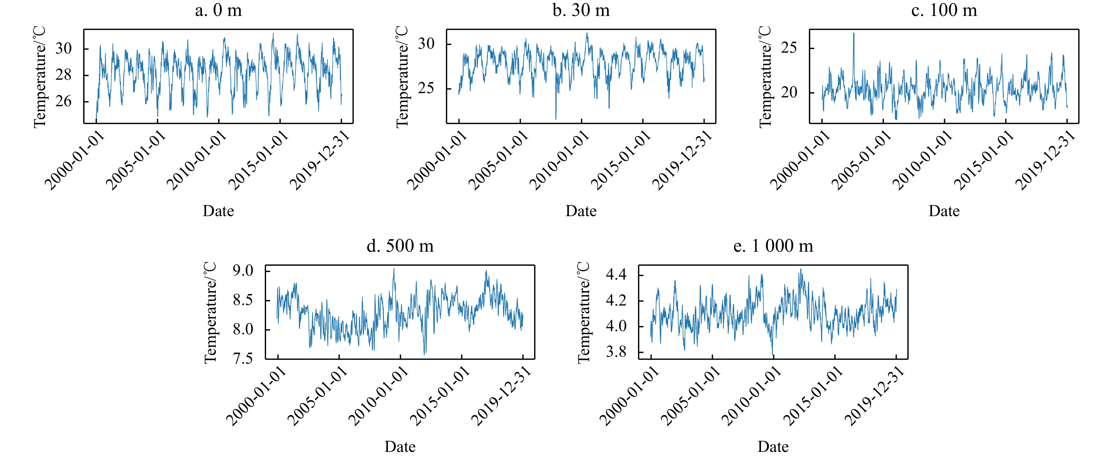
Figure 4. Seawater temperature trends at different depths at the same location (10°N, 111.25°E). Date format: YYYY-MM-DD.
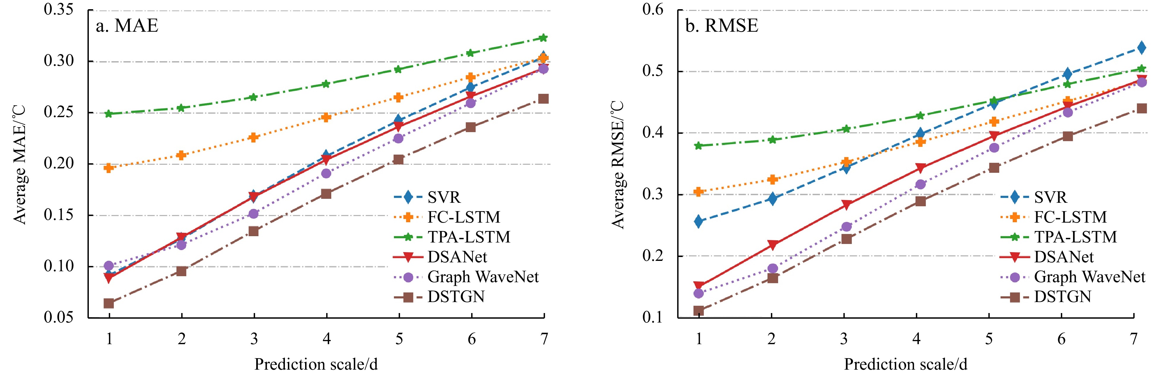
Figure 5. Comparison of the prediction results of different models.
Figure 6. Comparison of the prediction results of different models at different depths.
Figure 7. Fit plot of average temperature predictions (pred) at different depths. The blue curve represents the average actual temperature in the experimental area, and the orange curve represents the average predicted temperature in the corresponding area. Date format: YYYY-MM-DD.
Figure 8. Visualization of the 3D-OT distribution and the predicted results of DSTGN for different depth layers. “Tem_real” represents the true temperature, “Tem_DSTGN” represents the predicted temperature by DSTGN, and “Abs_error” represents the absolute error, which is defined as |Tem_DSTGN – Tem_real|.
Figure 9. Prediction error distributions of different models in different ocean temperature layers. The error plots of SVR, FC-LSTM, TPA-LSTM, DSANet, Graph WaveNet, and DSTGN are 0 m, 30 m, 100 m, 500 m, and 1 000 m under the sea from top to bottom. The color bar on the right represents the MAE value. The red circle area indicates that our model is significantly better than other models.
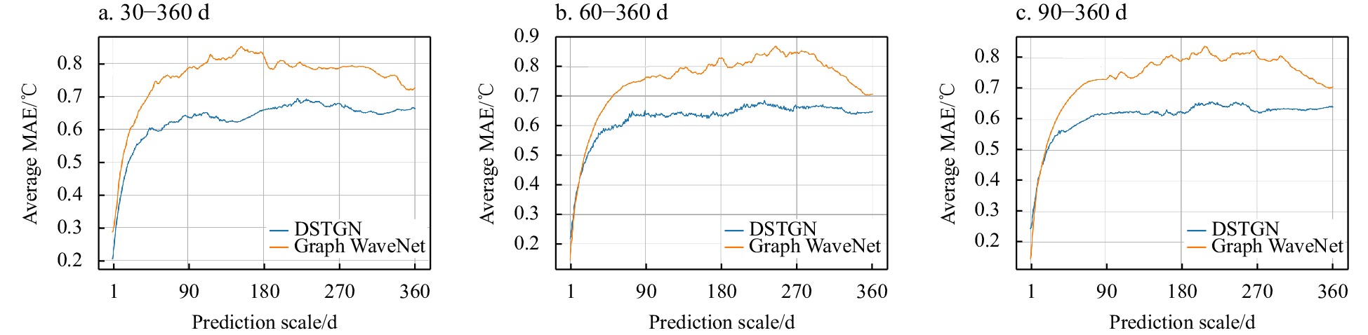
Figure 10. Prediction average MAE curves in different input windows.
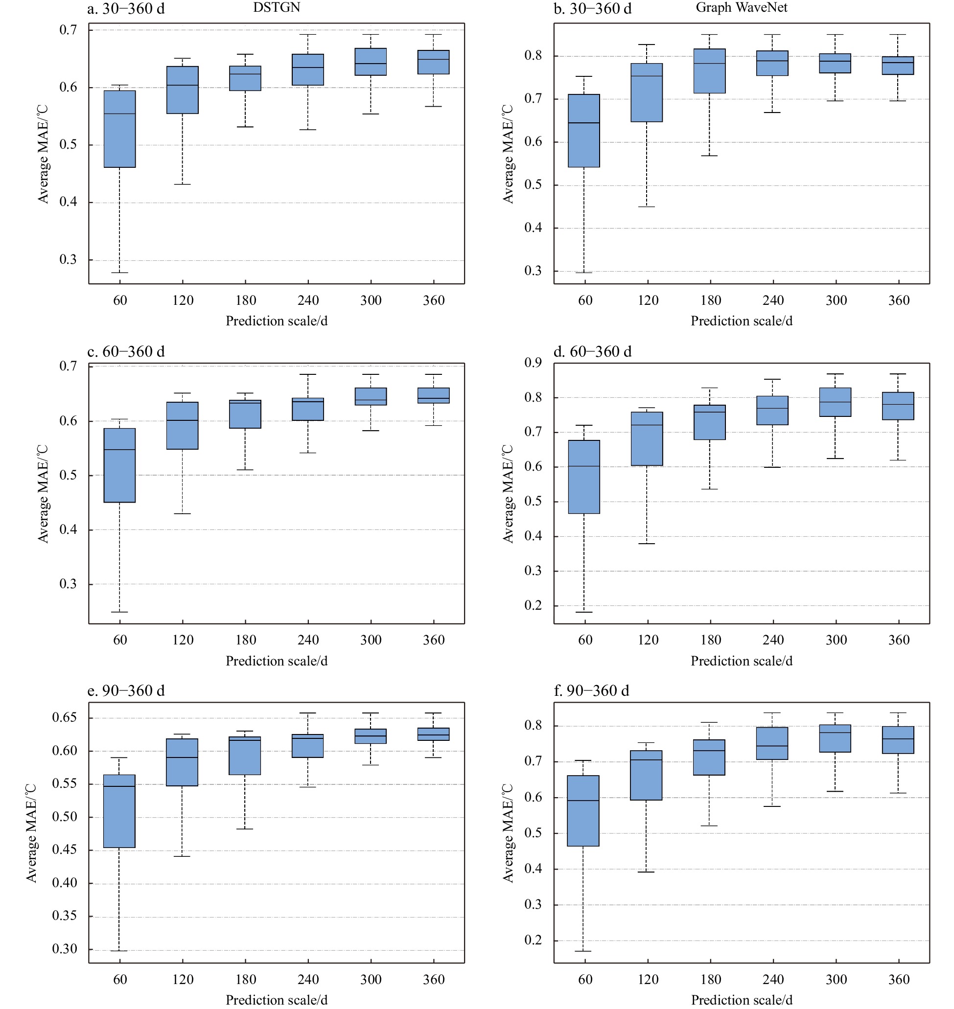
Figure 11. Boxplots of prediction average MAE with different output windows and input windows.
Figure 12. Pearson correlation coefficients for Points A, B, and C (shown in Fig. 1). The time range is from 1 January 2016 to 31 December 2019, the green curve represents the Pearson correlation coefficient for the true temperature and the red curve represents the Pearson correlation coefficient for the predicted values of the DSTGN. Data format: YYYY-MM-DD.


 DownLoad:


 DownLoad:


 DownLoad: