Ze Meng, Lei Zhou, Baosheng Li, Jianhuang Qin, Juncheng Xie. Erratum to: Acta Oceanologica Sinica (2022) 41(10): 119–130DOI: 10.1007/s13131-022-2023-3The atmospheric hinder for intraseasonal sea-air interaction over the Bay of Bengal during Indian summer monsoon in CMIP6[J]. Acta Oceanologica Sinica. doi: 10.1007/s13131-022-2131-0
Citation:
Xiaofan Hong, Zuozhi Chen, Jun Zhang, Yan’e Jiang, Yuyan Gong, Yancong Cai, Yutao Yang. Construction and analysis of a coral reef trophic network for Qilianyu Islands, Xisha Islands[J]. Acta Oceanologica Sinica, 2022, 41(12): 58-72. doi: 10.1007/s13131-022-2047-8
Key Laboratory for Sustainable Utilization of Open-sea Fishery of Ministry of Agriculture and Rural Affairs, South China Sea Fisheries Research Institute, Chinese Academy of Fishery Sciences, Guangzhou 510300, China
2.
Southern Marine Science and Engineering Guangdong Laboratory (Guangzhou), Guangzhou 511458, China
3.
College of Marine Sciences, Shanghai Ocean University, Shanghai 201306, China
Funds:
The National Key Research and Development Program of China under contract No. 2018YFC1406502; the National Natural Science Foundation of China under contract No. 31902374; the Key Special Project for Introduced Talents Team of Southern Marine Science and Engineering Guangdong Laboratory (Guangzhou) under contract No. GML2019ZD0605; the Central Public-Interest Scientific Institution Basal Research Fund of Chinese Academy of Fishery Sciences under contract No. 2020TD05.
Qilianyu Islands coral reefs (QICR), located in the northeastern part of the South China Sea, has been affected by human activities and natural disturbance. To characterize the trophic structure, ecosystem properties and keystone species of this region, a food-web model for the QICR is developed using methods involving a mass-balance approach with Ecopath with Ecosim software. Trophic levels range from 1.00 for detritus and primary producers to 3.80 for chondrichthyes. The mean trophic transfer efficiency for the entire ecosystem is 13.15%, with 55% of total energy flow originating from primary producers. A mixed trophic impact analysis indicates that coral strongly impacts most components of this ecosystem. A comparison of our QICR model with that for other coral reef ecosystems suggests that the QICR ecosystem is immature and/or is degraded.
Objective analysis, a kind of techniques for gridding observations, has developed and evolved for many decades. Historically, its main purpose is to provide initial conditions for operational prediction models and aid in the diagnostic studies in atmospheric and oceanic field. Although the use for the first purpose has all but disappeared today due to the springing-up of other more sophisticated schemes such as optimal interpolation (OI) and variational methods, objective analysis schemes are still widely used for diagnostic purposes and many studies have employed various incarnations of them to investigate a diverse range of researches.
As a branch of objective analysis, successive correction menthod (SCM) represented by Cressman (1959) and Barnes (1964, 1973) have received more attention than others and remain popular today. Cressman (1959) used a series of scans with decreasing radius of influence to retrieve a broad spectrum of wavelengths from the observations. Its major contribution is introducing the practice of building details from longer to shorter waves. Barnes (1964) argued that such a scheme suffered from the disadvantage of tending to smooth out all small variations in the field. Moreover, an unstable iteration may occur in the Cressman scheme and thus an additional dissipation scheme has to be performed (e.g., Seaman, 1983; Seaman and Hutchinson, 1985; Lu and Browning, 1998). To maximize details resolved by observations, Barnes (1964) proposed a scheme similar to the Cressman method but using a different weighting function (Gaussian-type) with the weight factor (radius of influence) fixed for all passes of scan. This algorithm was then replaced by Barnes (1973) employing only two passes (one initial pass and one correction pass) with a diminished smoothing factor for the second (correction) pass. The most attractive feature of the Barnes scheme is its well-known response characteristics. By choosing the smoothing parameters, one can ascertain which range of wavelengths will be retained in the final analysis. However, the response function of the Barnes (1964, 1973) is derived under the assumption that the observations are continuous and unbounded (infinite). Practically, it is best applicable to reasonably uniform data distributions. If data are irregularly distributed, the phase of the response function will change and signals may be distorted in the analyzed field. The more sparsely and irregularly distributed the data, the less results are in accordance with the theoretical predictions (Achtemeier, 1986; Pauley and Wu, 1990; Buzzi et al., 1991). This raises the difficulty of choosing the appropriate parameters in a particular application to achieve an optimum analysis. In fact, in the situation of sparse and irregular data distribution, no single selection of the parameters can produce the most accurate analysis for all wavelengths.
As we know, an effective objective analysis scheme should at least be able to retrieve resolvable long wavelengths in data-spare areas and preserve details in data-dense areas. If multi-wavelengths are extracted simultaneously without an effective mechanism, the analysis can be seriously contaminated by noises, arising from observational errors or irregular data distribution. A practical way to relieve this problem is analyzing first for larger scales and then for shorter scales. The more accurate the long wavelengths, the less impact the noises may have on the analyzed field. Therefore, when applied to irregularly spaced data, it is advisable for analysis scheme sequentially decrease the smoothing factors as Cressman method does in order to retain the most accurate analysis of the longer wavelengths. Based upon this idea, some variational successive corrections approaches, such as the multi-grid approach, the multi-scale diffusion filter approach, etc, have proposed by scholars as listed in Table 1. Among them, Xie et al. (2005, 2010) proposed a multi-scale 3D-VAR implemented by the multi-grid technique, using a sequence of grids with different resolutions to correct different wavelengths. The analysis is interpolated between two consecutive grid level and then enter into a new analysis cycle. Strictly speaking, the multi-grid 3D-VAR is not a traditional sense of 3D-VAR because it solves a series of 3D-VAR respectively on different grid levels. If the background filed is neglected and only the observational field is considered, the multi-grid 3D-VAR then evolves into a variational objective analysis scheme. Then one problem arise, is it possible for a variational objective analysis method to handle all spatial scales of observations in a single iterative procedure, rather than solve certain number of variational problems?
In this paper, a variant of SCM that can satisfy the above requirement, called SMRF, is proposed. Its main idea persists with other successive correction schemes in extracting multi-scale information from observations. Unlike these other schemes, it uses a variational optimization technique to minimize the difference between the estimated and the observed field. It is actually a combination of SCM and a minimization algorithm. We incorporate scales information into a minimization algorithm by using a recursive filter at each iteration to retrieve desired wavelengths successively. As a result, apart from the advantage in multi-scale information extraction, this scheme gains extra benefits from the minimization procedure: first, the inherent convergence property is guaranteed; second, the weighting parameters can be automatically determined by a line search algorithm without manual interventions; the last, it can analyze the data in all scales at one time.
The paper is organized as follows. The background knowledge related to the topic of this paper is briefed in Section 2, including the SCM and gradient-based minimization algorithms. In Section 3, in view of the relationship between the SCM and gradient-based minimization algorithms, the SMRF scheme is proposed by incorporating scales information into a minimization procedure. In Section 4, a single-observation experiment and an idealized SIC assimilation experiment are performed to evaluate the new scheme. The conclusions are summarized in Section 5.
2.
Necessary background
In this section, the SCM and the gradient-based minimization algorithms are briefly introduced.
2.1
Basics of SCM
The SCM is a kind of empirical approaches to correct the first-guess field by a linear combination of residual difference between the predicted and the observed values. In other words, the initial estimation field is gradually modified with the actual observation field until the correction factor is no greater than the given error value, at which time the revision process can be considered as the end. The formula is as follows:
where $ i,j $ is index of the analyzed grid point, the superscript $ n $ denotes the n-th iteration, $ {G}_{i,j}^{n} $is the analyzed value at the n-th iteration, and $ {G}_{i,j}^{0} $ corresponds to the first-guess field, $ {C}_{i,j}^{n} $ is the correction factor. The expression of correction factor is:
where $ M $ is the total number of observations within the circular areas of $ i,j $ point with radius $ R $, $ s $ denotes the s-th observation, $ {Q}_{s} $ is difference between the predictedand the observed values, and $ {W}_{s}^{n} $ is a weight function at the n-th iteration. The SCM can correct an analysis from longer to shorter wavelengths by changing the weight functions during iterations.
2.2
Basics of gradient-based minimization methods
The basic problem is to minimize a cost function as follows
$$
\min J\left(x\right),
$$
where $ x $ is the controlling variable, typically $ x\in {R}^{n} $, but this can also be subject to constraints. To numerically approximate the solution, a sequence $ {\left\{{x}_{n}\right\}}_{n=1}^{\infty } $ should be constructed so that $ {x}_{n} $→$ {x^*} $, where $ J\left({x^*}\right)=\rm{min}J\left(x\right) $. Many kinds of algorithms existed for this problem, one is known as gradient-based, in which the sequence $ {\left\{{x}_{n}\right\}}_{n=1}^{\infty } $ is constructed iteratively by choosing a search direction $ {p}_{n} $ at each iteration and minimizing $ J\left(x\right) $ along this direction. This reduces the problem essentially to a sequence of one-dimensional problem and $ {x}_{n} $ is given by the basic recurrence:
$$
{x}_{n+1}\!=\!{x}_{n}\!+\!{l}_{n}{p}_{n},
$$
(3)
where $ {l}_{n} $ is the step length, $ {p}_{n} $ is usually constructed using gradient information and we call $ {p}_{n} $ a descent direction if $\nabla {J}_{n}\!\cdot\! {p}_{n}\! < \! 0$, where $ \nabla J_n $ is the gradient of $ J $ with respect to $ x $ at $ {x}_{n} $. Based on the conjugate gradient optimization theory, $ {p}_{n} $ is fomulated as a product of $ \nabla J_n $ and a positive definite matrix $ {E}_{n} $, namely $ {p}_{n}\!=\!-{E}_{n}\nabla {J}_{n} $. If $ {E}_{n} $ is simplified to a unit matrix, Eq. (3) is the well-known steepest descent algorithm. Once the descent direction $ {p}_{n} $ is selected, the step length $ {l}_{n} $ can be determined through a line search algorithm (Moré and Thuente, 1994) to insure a sufficient decrease of the cost function along this direction.
3.
The SMRF scheme
To retrieve multi-scale information resolved by observations, a variant of SCM scheme using variational technique, called SMRF, is developed. It is a combination of SCM and minimization algorithms.
3.1
Similarities between the SCM and the minimization algorithm
Actually, the recursion formulated by Eq. (3) is also a procedure of successive correction. Considering the following problem that minimizes the difference between the estimated and the observed values
where $ x $ is the analyzed field, $ {x}^{{\rm{o}}} $ is the observed field, $ {{H}} $ is an interpolation operator from analysis space to observation space, $ {{R}} $ is the observational error covariance matrix, (·)T indicates transpose, and (·)–1 indicates inversion, the gradient of $ J\left(x\right) $ is:
Apparently, $ \nabla J\left(x\right) $ actually represents the residual difference between the observed value $ {x}^{{\rm{o}}} $ and the estimated value $ x $ on analysis grid. In Eq. (3), if we choose $ {p}_{n}=-{{{E}}}_{n}\nabla J\left({x}_{n}\right) $ ($ {{{E}}}_{n} $ is a positive definite matrix) as the descent direction, Eq. (3) becomes
where $ {w}_{n}={l}_{n}{{{E}}}_{n}{{{H}}}^{{\rm{T}}}{{{R}}}^{-1} $ is the weight for the $ n{\rm {-}}\rm{th} $ iteration. Equation (6) has the same form as the successive correction procedure except that the weights $ {w}_{n} $ are different and are obtained in different ways.
3.2
Problems with minimization algorithms
Once the gradient is obtained according to Eq. (5), the problem Eq. (4) then can be solved by using such a minimization algorithm as the steepest descent, the LBFGS, or the conjugate gradient method. However, this problem is usually ill-posed due to the scarcity and the irregular distribution of the observations. Further, without an effective mechanism of transmitting observational signals, the analysis will lose its coherent long-wave feature in data-void areas. From a minimization viewpoint, we will reveal in this portion that the underlying cause lies in the “flawed” gradient $ \nabla J\left(x\right) $ arising from the irregular data distribution.
For simplicity, $ {{R}} $ is assumed to be an identity matrix, Eq. (5) then becomes
Given $ n $ analyzed grid points and $ m $ observational locations, then $ x $ is a vector of length $ n $, $ {x}^{{\rm{o}}} $ is a vector of length $ m $. We also assume that the observations are right located at the analyzed grid points and $ m\!<\! n $. In such a case, the analyzed grid points can always be indexed by a certain order of observational locations so that $ {{H}} $ has the following form
Note that the last $ n{\rm{-}}m $ columns of $ {{H}} $ are all zero vectors. Accordingly, the last $ n{\rm{-}}m $ elements of $ {{{H}}}^{{\rm{T}}}\left({x}^{{\rm{o}}}\!-\!{{{H}}x}\right) $ are zero elements. As a result, for a grid point where no measurements are available, the corresponding element of $ {{{H}}}^{{\rm{T}}}\left({x}^{{\rm{o}}}\!-\!{{{H}}x}\right) $ at that position is definitely equal to zero, while for those observed grid points, the corresponding elements of $ {{{H}}}^{{\rm{T}}}\left({x}^{{\rm{o}}}\!-\!{{{H}}x}\right) $ remain their actual values. That is, the distribution of $ {{{H}}}^{{\rm{T}}}\left({x}^{{\rm{o}}}\!-\!{{{H}}x}\right) $, and thus $ \nabla J\left(x\right) $, is spatially incoherent. Though from a mathematical viewpoint, $ \nabla J\left(x\right) $ obtained in this way is unquestionable, this phenomenon is unreasonable in a physical sense because it is merely caused by the irregular data distribution.
If this “flawed” gradient is introduced into a general gradient-based minimization algorithm, it’s not strange that the analysis will deviate far from what we anticipate. Taking the steepest descent algorithm, for example, the estimate is updated at the $ i{\rm{-}}\rm{th} $ iteration by
As indicated above, $ \nabla J\left({x}_{0}\right) $ is spatially incoherent in data-void areas and therefore $ {x}_{1} $ will also involve amounts of erroneous small scales in these regions. The same issue runs through all later iterations, leading to a long-wave loss in data-void areas. As for those other gradient-based minimization algorithms, such as the LBFGS and the conjugate gradient method, the same problem exists, for a similar reason.
3.3
Variational form of SCM
Recognizing the defect of the conventional minimization algorithms in solving an ill-posed problem, and recalling the resemblance of a SCM and a minimization algorithm, we are enlightened to refer to the desirable feature of a SCM scheme in multi-scale analyzing and incorporate it into a minimization algorithm. We apply a recursive filter to the gradient of the cost function at each iteration of a minimization procedure. With the filter parameter decreasing sequentially with iterations, various scales, from longer to shorter wavelengths, can be extracted successively (see Appendix for recursion details).
We now give a brief analysis on the fundamentals of this scheme. The gradient $ \nabla J\left(x\right) $ described by Eq. (5) actually represents observational residuals at $ x $. The scheme starts by applying a recursive filter E to $ -\nabla J\left({x}_{0}\right) $ with a large enough $ \alpha $, resultant $ {{E}}\left(-\nabla J\left({x}_{0}\right)\right) $ then reasonably characterizes the “longest” wavelengths of the observational residuals at $ {x}_{0} $. Also, since the recursive filtering operator E is positive definite, $ {{E}}\left(-\nabla J\left({x}_{0}\right)\right) $ is guaranteed to be a descent direction which insures the decrease of the residual difference between the estimated and the observed values along this direction. However, just as what we have depicted in the first part of Appendix, for any wavelength the filtering process of $ {{E}}\left(-\nabla J\left({x}_{0}\right)\right) $ will lead to some amplitude loss. A reasonable analysis over data-sparse areas requires the long waves be captured as accurately as possible so that it will not interfere with the extraction of shorter wavelengths in later iterations. Therefore, to regain some of those lost information, a line search procedure is performed along this direction to find an appropriate step length $ l $. When the estimate is updated by $ {x}_{1}\!=\!{x}_{0}\!+\! l{{E}}\left(-\nabla J\left({x}_{0}\right)\right) $, the “largest” scale of the observational residuals at $ x\!=\!{x}_{0} $ is “fully” extracted and incorporated into the new estimate $ {x}_{1} $. Then $ \alpha $ is diminished appropriately, as a result, the “largest” scale of the observational residuals at $ x\!=\!{x}_{1} $ can be captured at the second iteration and incorporated into $ {x}_{2} $. As iteration proceeds, all scales, from longer to shorter wavelengths, can be pulled out successively.
Actually, this scheme is a natural extension of the Barnes SCM scheme (Barnes, 1964, 1973). But it is in a variational form with the advantage that the weights can be automatically obtained by a line search algorithm. This scheme can also be regarded as a minimization algorithm which gains an advantage over conventional minimization algorithms by accounting for various spatial scales resolved by the observations.
To further suppress observational noises, we make a slight modification to our scheme by replacing the problem described by Eq. (4) with the following:
where $ {{B}} $ is another recursive filtering operator with a very small filter parameter $ \,\beta $. Obviously, problem Eq. (4) is the special case of Eq. (10) when $ \, \beta \!=\! 0 $. For the same reason as we have explained, solving Eq. (10) directly using a conventional minimization algorithm (e.g., the steepest descent, the LBFGS and the conjugate gradient method) may not yield a well-behaved analysis, as is verified by our experiments in Section 4. Our algorithm is modified as a flow chart shown in Fig. 1.
It should be noted that the cost function defined by Eq. (10) is a counter part of that used in a 3D-VAR, representing the observational term. Therefore, the way we used in analyzing for the gradient is also suitable for a 3D-VAR scheme, see Appendix for details.
4.
Experiment designs and results
4.1
Single-observation experiment
An effective mechanism for transmitting observational information should be able to: (1) insure the accuracy of the analysis. (2) make observational signals propagate to more wide areas so that the analysis for long waves can be dramatically improved in data-sparse or data-void regions. To test the ability of the SMRF scheme, two experiments are carried out using a single observation. In the first experiment, the recursive filtering operator B with an invariant filter parameter $\, \beta $ is applied to the w and Eq. (10) is directly solved using a conventional LBFGS minimization algorithm (Liu and Nocedal, 1989). In the second experiment, another recursive filtering operator E with variable filter parameters is applied to the cost function gradient $ -\nabla J\left(w\right) $ besides the recursive filtering operator B is applied to w, and Eq. (10) is solved using the SMRF scheme, as shown in Fig. 1.
4.1.1
Data and parameters
The analysis domain covers a square region, extending 10˚ both in latitude and in longitude. The grid resolution is 0.25˚×0.25˚. We place only one observation with its value equal to 1.0 at the center of this domain. The number of filtering passes $ M $ is set to 8. The filer parameter $ \alpha $ in our scheme is chosen as the following Gaussian function:
$$
\alpha \!=\!{\alpha }_{\rm{max}}\!\cdot\! {{\rm{e}}}^{-\frac{{i}^{2}}{2{\sigma }^{2}}},\qquad i\!=\!0,1,\cdots, N,
$$
(11)
where $ i $ represents the iteration number, $ N $ is a constant to be set, $ \sigma \!=\!\dfrac{N}{4} $, $ {\alpha }_{\rm{max}}\!=\! 0\rm{.999} $. As we can see, at the beginning, $ \alpha \!=\!{\alpha }_{\rm{max}} $$\left(i\!=\! 0\right)$, then $ \alpha $ decreases with iterations and almost approaches zero (exactly, $ {{\rm{e}}}^{-8} $) when $ i\!=\! N $, so the number of iterations can be chosen to be no greater than $ N $ in practical implementations. In this experiment we set $ N\!=\! $250. The observation operator $ {{H}} $ is a simple bilinear interpolation. The initial-guess field $ {w}_{0} $ is selected to be zero. The line search algorithm is based on the study by Moré and Thuente (1994).
4.1.2
Results
Figure 2 shows the results of solving Eq. (10) by the LBFGS algorithm when filter parameter $\, \beta $=0.1 and 0.4, respectively. As can be seen, since a recursive filter makes grid points connect and interact with each other, even a single observation can transmit observational signals to neighboring grid points. Different choice of $ \,\beta $ will yield different analysis. If $\, \beta $ is relatively large, the observational signals can propagate to more wide range of areas, but the analysis will lose accuracy in practical use. If $\, \beta $ is small (e.g., $\, \beta $=0.1), the analysis approaches the observation closely but remains all most unchanged in data-void regions because observational signals cannot propagate there. Thus, maximizing the details requires a small $\, \beta $ and filling in the data-void areas with long waves needs a large $\, \beta $. It seems that there is no way to take care of both of these two aspects simultaneously. However, this can to some extent be remedied by our scheme.
Figure
2.
The spread of observational information using the LBFGS algorithm when β=0.1 (a) and β=0.4 (b).
Figure 3 tells the results of the SMRF scheme at different iterations using a small filter parameter $\, \beta $(=0.1). Figures 3a, b, c and d are for iteration 50, 100, 130, and 180, respectively. Apparently, the analysis is corrected from large scales to details. As a result, observational signals can propagate to more wide regions while at the same time the analysis does not lose its accuracy. For a further understanding of the evolving process of our analysis with iterations, the surface plots of Figs 2a and 3 are presented as Figs 4 and 5 respectively. Figure 4 shows that using the LBFGS algorithm with a small $ \,\beta $(=0.1), while the accuracy is guaranteed near the observed locations, the observation can only have an effect on a very close area around it. Figure 5 depicts that in the SMRF scheme, with the same small $\, \beta $(=0.1), the analysis starts with a coarse field and approaches the observed value gradually, and the observational signals can be transmitted to more wide areas compared with that in Fig. 4.
Figure
3.
The spread of the observational information in the SMRF scheme when β=0.1. a, b, c and d. The results at iteration 50, 100, 130 and 180, respectively.
For further verifying the effectiveness of the SMRF scheme in extracting spatial multi-scale information, a two-dimensional experiment with SSMI SIC observations is carried out. To reveal how different wavelengths are corrected sequentially, the analyzed field and the descent direction at different iterations in the SMRF scheme are explored in comparison with the counterparts solved by using the steepest descent algorithm.
4.2.1
Data and parameters
The SSMI daily SIC data are obtained from the National Snow and Ice Data Center (NSIDC), the horizontal resolution of which is 25 km × 25 km. The analysis domain covers the Arctic Ocean. The “true” state of SIC field is shown in Fig. 6a, which is constructed by the SIC observations from the SSMI on September 1, 2014. Since the spatial resolution of the analysis field is usually different from the satellite observation, we select one observation for every four analysis grid points. We also remove partial points located in the sea ice marginal ice zone to examine the validation of the SMRF scheme. As a consequence, there are 1 384 observations (Fig. 6b) remained to restore the “true” field. The observation errors are assumed to be uncorrelated and therefore a diagonal matrix is used with all diagonal elements equal to the square of the observation standard deviation, $ {\sigma }_{{\rm{o}}}^{2} $. $ {\sigma }_{{\rm{o}}} $ here has been normalized to 1.0 in order to avoid the complexity. $ \,\beta $ is chosen to be 0.2. $ N $ is set to 500. The other settings remain the same as those in the single-observation experiment above.
Figure
6.
The true SIC field of Arctic Ocean constructed based on the SSMI SIC on September 1, 2014 (a); and the locations of “observations” (b).
As can be seen from Fig. 7, the analysis results constructed by the steepest descent algorithm deeply rely on $ \,\beta $. The small (large) $ \beta $, which is related to the small (large) radius of influence, only reflects the short (long) wave information of the observations, indicating the long and short wave information cannot be resolved simultaneously. Figure 8 shows results of the steepest descent algorithm with $ \, \beta\! = $0.2 at iteration 3, 5 and 7. The descent direction is spatially incoherent in the data-void region because of the sharp variation of the gradient caused by the irregular distribution of observations (Figs 8b, d and f). Accordingly, there analysis updated along this direction tend to the incoherent structure (Figs 8a, c and e). The same problem will exist for other gradient-based minimization algorithms such as the quasi-Newton methods, LBFGS and the conjugate gradient method.
Figure
7.
Analyzed field solved by using the steepest descent algorithm β=0.2 (a), β=0.4 (b), β=0.6 (c) and β=0.8 (d), in which the iteration is 25, 162, 165 and 148, respectively.
Figure
8.
Analyzed field (left column) and the descent direction ($ -\nabla J $) (right column) solved using the steepest descent algorithm ($ \beta $=0.2) at iteration 3, 5 and 7, respectively.
The analysis results from SMRF scheme with $ \beta \!= $0.2 is very similar with the true field (Fig. 9), which avoids the incoherent spatial structure in the data-void area compared to the steepest descent algorithm. Therefore, the SMRF scheme can better account for various spatial scales resolved by the observations, and the long and short wavelength information can be extracted simultaneously from the observations (Figs 10a, c and e). This is attributed to the fact that the descent direction is built by smoothing out the sharp variation of the gradient to extract the long wave of the observational residuals. As the filtering scales $ \alpha $ decreases with iterations, the descent direction is obtained from longer to shorter wavelengths (Figs 10b, d and f). Consequently, the analyzed field adjusted along this direction can also be extracted successively.
Figure
9.
The true SIC (a) and the analysis result (b) from the SMRF scheme with β=0.2 and N=500.
Ideally, $ \alpha $ should decrease continuously with iterations. However, discrete ones are needed in practical implementations. As $ \alpha $ takes the form of Eq. (11) in our scheme, the choice of $ N $ is an issue to be considered. Figure 11 gives the analysis results with different value of $ N $. As can be seen, the desirable analysis can be achieved as $ N\!>\!\rm{15}0 $ in this experiment. It is also shown in our other experiments that the choice of $ N $ is not a problem in practice because we can usually achieve reasonable results as long as $ N $ is big enough. However, too big value is not necessary and also not recommended because of the computational cost.
Figure
11.
Analysis of the SMRF scheme (β=0.2) with different choice of N. a. b. c and d. N=10, 20, 150 and 300, respectively.
In this study, a muti-scale variational optimization technique is designed to extract spatial multi-scale information resolved by observations. In view of the similarity in form between the SCM schemes and the gradient-based algorithms, the new approach incorporates scales into the minimization algorithms. Additionally, to propagate observational signals, it applies recursive filters to the gradient of the cost function and makes filtering scales decrease with iterations to extract various scales. Based on SRMF scheme, the SIC analysis fields can be successfully reconstructed through extracting the information of the real SSMI from long to short waves in turn.
The main conclusions can be summarized as follows.
(1) This scheme is a variant of conventional SCM that can better account for resolvable multi-scale in the observations. Actually, it is a natural extension of the Barnes scheme but in a variational form, which brings us several extra benefits. First, the specification of scheme parameters is relatively easy because the weights are automatically determined by a line search algorithm. Second, the convergence is implied in a minimization procedure and the “distance” between the estimate and the observed value is diminished with iterations. The last, all wavelengths are analyzed at one time in a single iterative procedure.
(2) From a physical viewpoint, the spatial distribution of the gradient of a cost function defined in a variational problem may be unreasonable, for example, in condition that data are irregularly distributed. Use of this gradient in a conventional minimization algorithm (e.g., the steepest descent, the LBFGS, or the conjugate gradient method) will cause a poor analysis. Our scheme is a remedial approach for this issue. Though inter-comparison studies are performed in our experiments between the conventional minimization algorithms and the SMRF scheme, this is not our real purpose because it is unfair for these algorithms in solving an ill-conditioned problem. On the contrary, we simply intend to present the feasibility and the effectiveness of the combination of SCM and a minimization procedure in data-spare cases.
(3) Since the cost function defined by Eq. (10) is a counter part of that used in a 3D-VAR, representing the observational term, the problem mentioned in (2) also exists in a 3D-VAR scheme if the background error covariance matrix is not appropriately modeled, which shows the potentiality of the SMRF scheme to be extended to a 3D-VAR, as will be detailed in Appendix.
(4) SMRF aims to capture longer wavelengths as accurate as possible before analyzing for shorter wavelengths. While this can to some extent reduce the chance of the long waves being contaminated by noises, there is no way to completely avoid this. How much noise contamination is included in an analysis and how much the signals are distorted is still a question to be studied, especially with a quantitative analysis. Additionally, compared with the multi-grid method (Xie et al., 2010), the computational cost is a defect of SMRF, and further improvements are needed.
(5) The high-order recursive filter can effectively avoid the problems such as large truncation error and difficult boundary estimation caused by the cascade of first-order recursive filter used in our study. The high-order recursive filter algorithm will be enclosed in the SMRF in the future. Besides, It will be further investigated to what degree the SMRF can improve the sea ice weather forecast precision and climate prediction skill.
A1.
Response functions of the recursive filter with different value of $ \alpha $.
Adey W H, Goertemiller T. 1987. Coral reef algal turfs: master producers in nutrient poor seas. Phycologia, 26(3): 374–386. doi: 10.2216/i0031-8884-26-3-374.1
Ainsworth C H, Mumby P J. 2015. Coral–algal phase shifts alter fish communities and reduce fisheries production. Global Change Biology, 21(1): 165–172. doi: 10.1111/gcb.12667
Albouy C, Mouillot D, Rocklin D, et al. 2010. Simulation of the combined effects of artisanal and recreational fisheries on a Mediterranean MPA ecosystem using a trophic model. Marine Ecology Progress Series, 412: 207–221. doi: 10.3354/meps08679
Allen K R. 1971. Relation between production and biomass. Journal of the Fisheries Research Board of Canada, 28(10): 1573–1581. doi: 10.1139/f71-236
Alva-Basurto J C, Arias-González J E. 2014. Modelling the effects of climate change on a Caribbean coral reef food web. Ecological Modelling, 289: 1–14. doi: 10.1016/j.ecolmodel.2014.06.014
Anthony K R N, Kline D I, Diaz-Pulido G, et al. 2008. Ocean acidification causes bleaching and productivity loss in coral reef builders. Proceedings of the National Academy of Sciences of the United States of America, 105(45): 17442–17446. doi: 10.1073/pnas.0804478105
Arias-González J E, Delesalle B, Salvat B, et al. 1997. Trophic functioning of the Tiahura reef sector, Moorea Island, French Polynesia. Coral Reefs, 16(4): 231–246. doi: 10.1007/s003380050079
Arias-González J E, Nuñez-Lara E, González-Salas C, et al. 2004. Trophic models for investigation of fishing effect on coral reef ecosystems. Ecological Modelling, 172(2–4): 197–212,
Bahr K D, Rodgers K S, Jokiel P L, et al. 2020. Pulse sediment event does not impact the metabolism of a mixed coral reef community. Ocean & Coastal Management, 184: 105007. doi: 10.1016/j.ocecoaman.2019.105007
Baums I B. 2008. A restoration genetics guide for coral reef conservation. Molecular Ecology, 17(12): 2796–2811. doi: 10.1111/j.1365-294X.2008.03787.x
Bello-Pineda J, Ponce-Hernández R, Liceaga-Correa M A. 2006. Incorporating GIS and MCE for suitability assessment modelling of coral reef resources. Environmental Monitoring and Assessment, 114(1–3): 225–256,
Bellwood D R, Hughes T P, Folke C, et al. 2004. Confronting the coral reef crisis. Nature, 429(6994): 827–833. doi: 10.1038/nature02691
Botha E J, Brando V E, Anstee J M, et al. 2013. Increased spectral resolution enhances coral detection under varying water conditions. Remote Sensing of Environment, 131: 247–261. doi: 10.1016/j.rse.2012.12.021
Bozec Y M, Gascuel D, Kulbicki M. 2004. Trophic model of lagoonal communities in a large open atoll (Uvea, Loyalty Islands, New Caledonia). Aquatic Living Resources, 17(2): 151–162. doi: 10.1051/alr:2004024
Bozec Y M, O’Farrell S, Bruggemann J H, et al. 2016. Tradeoffs between fisheries harvest and the resilience of coral reefs. Proceedings of the National Academy of Sciences of the United States of America, 113(16): 4536–4541. doi: 10.1073/pnas.1601529113
Brandl S J, Emslie M J, Ceccarelli D M, et al. 2016. Habitat degradation increases functional originality in highly diverse coral reef fish assemblages. Ecosphere, 7(11): e01557. doi: 10.1002/ecs2.1557
Brown P C, Painting S J, Cochrane K L. 1991. Estimates of phytoplankton and bacterial biomass and production in the northern and southern Benguela ecosystems. South African Journal of Marine Science, 11(1): 537–564. doi: 10.2989/025776191784287673
Cáceres I, Ortiz M, Cupul-Magaña A L, et al. 2016. Trophic models and short-term simulations for the coral reefs of Cayos Cochinos and Media Luna (Honduras): a comparative network analysis, ecosystem development, resilience, and fishery. Hydrobiologia, 770(1): 209–224. doi: 10.1007/s10750-015-2592-7
Cheal A J, MacNeil M A, Cripps E, et al. 2010. Coral–macroalgal phase shifts or reef resilience: links with diversity and functional roles of herbivorous fishes on the Great Barrier Reef. Coral Reefs, 29(4): 1005–1015. doi: 10.1007/s00338-010-0661-y
Chen Zuozhi, Qiu Yongsong. 2010. Assessment of the food-web structure, energy flows, and system attribute of northern South China Sea ecosystem. Acta Ecologica Sinica, 30(18): 4855–4865
Chen Zuozhi, Xu Shannan, Qiu Yongsong. 2015. Using a food-web model to assess the trophic structure and energy flows in Daya Bay, China. Continental Shelf Research, 111: 316–326. doi: 10.1016/j.csr.2015.08.013
Chen Xiaoyan, Yu Kefu, Huang Xueyong, et al. 2019. Atmospheric nitrogen deposition increases the possibility of macroalgal dominance on remote coral reefs. Journal of Geophysical Research: Biogeosciences, 124(5): 1355–1369. doi: 10.1029/2019jg005074
Chen Biao, Yu Kefu, Liao Zhiheng, et al. 2021. Microbiome community and complexity indicate environmental gradient acclimatisation and potential microbial interaction of endemic coral holobionts in the South China Sea. Science of the Total Environment, 765: 142690. doi: 10.1016/j.scitotenv.2020.142690
Chesher R H. 1969. Destruction of Pacific corals by the sea star Acanthaster planci. Science, 165(3890): 280–283. doi: 10.1126/science.165.3890.280
Chong-Seng K M, Nash K L, Bellwood D R, et al. 2014. Macroalgal herbivory on recovering versus degrading coral reefs. Coral Reefs, 33(2): 409–419. doi: 10.1007/s00338-014-1134-5
Christensen V, Pauly D. 1992. ECOPATH II—a software for balancing steady-state ecosystem models and calculating network characteristics. Ecological Modelling, 61(3–4): 169–185,
Christensen V, Walters C J. 2004. Ecopath with Ecosim: methods, capabilities and limitations. Ecological Modelling, 172(2–4): 109–139,
Christensen V, Walters C J, Pauly D. 2005. Ecopath with Ecosim: A User’s Guide. Vancouver: University of British Columbia
Christensen V, Walters C, Pauly D, et al. 2008. Ecopath with Ecosim Version 6 User Guide. Vancouver: University of British Columbia
Cook C B, Logan A, Ward J, et al. 1990. Elevated temperatures and bleaching on a high latitude coral reef: the 1988 Bermuda event. Coral Reefs, 9(1): 45–49. doi: 10.1007/BF00686721
Darling E S, D’Agata S. 2017. Coral reefs: fishing for sustainability. Current Biology, 27(2): R65–R68. doi: 10.1016/j.cub.2016.12.005
Darnell R M. 1967. Organic detritus in relation to the estuarine ecosystem. In: Lauff G H, ed. Estuaries. Washington: American Association for the Advancement of Science, 376–382
Dove S G, Brown K T, Van Den Heuvel A, et al. 2020. Ocean warming and acidification uncouple calcification from calcifier biomass which accelerates coral reef decline. Communications Earth & Environment, 1(1): 55. doi: 10.1038/s43247-020-00054-x
Du Jianguo, Makatipu P C, Tao L S R, et al. 2020. Comparing trophic levels estimated from a tropical marine food web using an ecosystem model and stable isotopes. Estuarine, Coastal and Shelf Science, 233: 106518,
Du Feiyan, Wang Xuehui, Lin Zhaojin. 2015. The characteristics of summer zooplankton community in the Meiji coral reef, Nansha Islands, South China Sea. Acta Ecologica Sinica, 35(4): 1014–1021
Eyre B D, Cyronak T, Drupp P, et al. 2018. Coral reefs will transition to net dissolving before end of century. Science, 359(6378): 908–911. doi: 10.1126/science.aao1118
Fabricius K E, Okaji K, De’ath G. 2010. Three lines of evidence to link outbreaks of the crown-of-thorns seastar Acanthaster planci to the release of larval food limitation. Coral Reefs, 29(3): 593–605. doi: 10.1007/s00338-010-0628-z
Ferrier-Pagès C, Hoogenboom M, Houlbrèque F. 2011. The role of plankton in coral trophodynamics. In: Dubinsky Z, Stambler N, eds. Coral Reefs: An Ecosystem in Transition. Dordrecht: Springer,
Finn J T. 1976. Measures of ecosystem structure and function derived from analysis of flows. Journal of Theoretical Biology, 56(2): 363–380. doi: 10.1016/S0022-5193(76)80080-X
Fox H E, Caldwell R L. 2006. Recovery from blast fishing on coral reefs: a tale of two scales. Ecological Applications, 16(5): 1631–1635. doi: 10.1890/1051-0761(2006)016[1631:RFBFOC]2.0.CO;2
Frank K T, Petrie B, Shackell N L. 2007. The ups and downs of trophic control in continental shelf ecosystems. Trends in Ecology & Evolution, 22(5): 236–242. doi: 10.1016/j.tree.2007.03.002
Gaither M R, Bowen B W, Bordenave T R, et al. 2011. Phylogeography of the reef fish Cephalopholis argus (Epinephelidae) indicates Pleistocene isolation across the Indo-Pacific Barrier with contemporary overlap in the Coral Triangle. BMC Evolutionary Biology, 11: 189. doi: 10.1186/1471-2148-11-189
Gates R D. 1990. Seawater temperature and sublethal coral bleaching in Jamaica. Coral Reefs, 8(4): 193–197. doi: 10.1007/BF00265010
Glynn P W, Enochs I C. 2011. Invertebrates and their roles in coral reef ecosystems. In: Dubinsky Z, Stambler N, eds. Coral Reefs: An Ecosystem in Transition. Dordrecht: Springer, 273–325
Godinot C, Houlbrèque F, Grover R, et al. 2011. Coral uptake of inorganic phosphorus and nitrogen negatively affected by simultaneous changes in temperature and pH. PLoS ONE, 6(9): e25024. doi: 10.1371/journal.pone.0025024
González-Rivero M, Bongaerts P, Beijbom O, et al. 2014. The catlin seaview survey-kilometre-scale seascape assessment, and monitoring of coral reef ecosystems. Aquatic Conservation: Marine and Freshwater Ecosystems, 24(S2): 184–198. doi: 10.1002/aqc.2505
Heenan A, Williams I D, Acoba T, et al. 2017. Long-term monitoring of coral reef fish assemblages in the western central Pacific. Scientific Data, 4: 170176. doi: 10.1038/sdata.2017.176
Heymans J. 2003. Comparing the Newfoundland marine ecosystem models using Information Theory. Fisheries Centre Research Reports, 11(5): 62–71
Heymans J J, Coll M, Libralato S, et al. 2011. Ecopath theory, modeling, and application to coastal ecosystems. Treatise on Estuarine and Coastal Science, 9: 93–113
Heymans J J, Coll M, Link J S, et al. 2016. Best practice in Ecopath with Ecosim food-web models for ecosystem-based management. Ecological Modelling, 331: 173–184. doi: 10.1016/j.ecolmodel.2015.12.007
Hixon M A, Randall J E. 2019. Coral reef fishes. Encyclopedia of Ocean Sciences, 2: 142–150
Hodgson G. 1999. A global assessment of human effects on coral reefs. Marine Pollution Bulletin, 38(5): 345–355. doi: 10.1016/S0025-326X(99)00002-8
Hoegh-Guldberg O, Mumby P J, Hooten A J, et al. 2007. Coral reefs under rapid climate change and ocean acidification. Science, 318(5857): 1737–1742. doi: 10.1126/science.1152509
Houlbrèque F, Tambutté E, Ferrier-Pagès C. 2003. Effect of zooplankton availability on the rates of photosynthesis, and tissue and skeletal growth in the scleractinian coral Stylophora pistillata. Journal of Experimental Marine Biology and Ecology, 296(2): 145–166. doi: 10.1016/S0022-0981(03)00259-4
Huang Zirong, Chen Zuozhi, Zeng Xiaoguang. 2009. Species composition and resources density of Chondrichthyes in the continental shelf of northern South China Sea. Journal of Oceanography in Taiwan Strait, 28(1): 38–44
Huang Danwei, Licuanan W Y, Hoeksema B W, et al. 2015. Extraordinary diversity of reef corals in the South China Sea. Marine Biodiversity, 45(2): 157–168. doi: 10.1007/s12526-014-0236-1
Huang Jianhong, Wang Fengxia, Zhao Hongwei, et al. 2020. Reef benthic composition and coral communities at the Wuzhizhou Island in the South China Sea: the impacts of anthropogenic disturbance. Estuarine, Coastal and Shelf Science, 243: 106863,
Huang Hui, Zhang Chenglong, Yang Jianhui, et al. 2012. Scleractinian coral community characteristics in Zhubi reef sea area of Nansha Islands. Journal of Oceanography in Taiwan Strait, 31(1): 79–84
Hughes T P, Rodrigues M J, Bellwood D R, et al. 2007. Phase shifts, herbivory, and the resilience of coral reefs to climate change. Current Biology, 17(4): 360–365. doi: 10.1016/j.cub.2006.12.049
Ippolito S, Naudot V, Noonburg E G. 2016. Alternative stable states, coral reefs, and smooth dynamics with a kick. Bulletin of Mathematical Biology, 78(3): 413–435. doi: 10.1007/s11538-016-0148-2
Jiao Nianzhi, Chen Dake, Luo Yongming, et al. 2015. Climate change and anthropogenic impacts on marine ecosystems and countermeasures in China. Advances in Climate Change Research, 6(2): 118–125. doi: 10.1016/j.accre.2015.09.010
Jokiel P L. 2016. Predicting the impact of ocean acidification on coral reefs: evaluating the assumptions involved. ICES Journal of Marine Science, 73(3): 550–557. doi: 10.1093/icesjms/fsv091
Karim E, Liu Qun, Xue Ying, et al. 2019. Trophic structure and energy flow of the resettled maritime area of the Bay of Bengal, Bangladesh through ECOPATH. Acta Oceanologica Sinica, 38(10): 27–42. doi: 10.1007/s13131-019-1423-5
Ke Zhixin, Tan Yehui, Huang Liangmin, et al. 2018. Spatial distribution patterns of phytoplankton biomass and primary productivity in six coral atolls in the central South China Sea. Coral Reefs, 37(3): 919–927. doi: 10.1007/s00338-018-1717-7
Kim T W, Lee K, Duce R, et al. 2014. Impact of atmospheric nitrogen deposition on phytoplankton productivity in the South China Sea. Geophysical Research Letters, 41(9): 3156–3162. doi: 10.1002/2014gl059665
Landi P, Minoarivelo H O, Brännström Å, et al. 2018. Complexity and stability of ecological networks: a review of the theory. Population Ecology, 60(4): 319–345. doi: 10.1007/s10144-018-0628-3
Li Yuanjie, Chen Zuozhi, Zhang Jun, et al. 2020. Species and taxonomic diversity of Qilianyu Island reef fish in the Xisha Islands. Journal of Fishery Sciences of China, 27(7): 815–823
Li Yuanchao, Chen Shiquan, Zheng Xinqing, et al. 2018. Analysis of the change of hermatypic corals in Yongxing Island and Qilianyu Island in nearly a decade. Haiyang Xuebao (in Chinese), 40(8): 97–109
Li Yuanchao, Liang Jilin, Wu Zhongjie, et al. 2019a. Outbreak and prevention of Acanthaster planci. Ocean Development and Management, 36(8): 9–12
Li Xiong, Wang Hao, Zhang Zheng, et al. 2014. Mathematical analysis of coral reef models. Journal of Mathematical Analysis and Applications, 416(1): 352–373. doi: 10.1016/j.jmaa.2014.02.053
Li Yuanchao, Wu Zhongjie, Chen Shiquan, et al. 2017. Discussion of the diversity of the coral reef fish in the shallow reefs along the Yongxing and Qilianyu Island. Marine Environmental Science, 36(4): 509–516
Li Yuanchao, Wu Zhongjie, Liang Jilin, et al. 2019b. Analysis on the outbreak period and cause of Acanthaster planci in Xisha Islands in recent 15 years. Chinese Science Bulletin, 64(33): 3478–3484. doi: 10.1360/tb-2019-0152
Libralato S, Christensen V, Pauly D. 2006. A method for identifying keystone species in food web models. Ecological Modelling, 195(3–4): 153–171,
Lindeman R L. 1942. The trophic-dynamic aspect of ecology. Ecology, 23(4): 399–417. doi: 10.2307/1930126
Link J S. 2010. Adding rigor to ecological network models by evaluating a set of pre-balance diagnostics: a plea for PREBAL. Ecological Modelling, 221(12): 1580–1591. doi: 10.1016/j.ecolmodel.2010.03.012
Liu P J, Shao K T, Jan R Q, et al. 2009. A trophic model of fringing coral reefs in Nanwan Bay, southern Taiwan suggests overfishing. Marine Environmental Research, 68(3): 106–117. doi: 10.1016/j.marenvres.2009.04.009
Lough J M. 2011. Climate change and coral reefs. In: Hopley D, ed. Encyclopedia of Modern Coral Reefs. Encyclopedia of Earth Sciences Series. Dordrecht: Springer,
Luo Zhongyuan, Li Jiangtao, Jia Guodong. 2019. The geochemical significance of deep-water coral and their food source. Advances in Earth Science, 34(12): 1234–1242. doi: 10.11867/j.issn.1001-8166.2019.12.1234
MacNeil M A, Graham N A J, Cinner J E, et al. 2015. Recovery potential of the world’s coral reef fishes. Nature, 520(7547): 341–344. doi: 10.1038/nature14358
Mak K K W, Yanase H, Renneberg R. 2005. Cyanide fishing and cyanide detection in coral reef fish using chemical tests and biosensors. Biosensors and Bioelectronics, 20(12): 2581–2593. doi: 10.1016/j.bios.2004.09.015
Mantyka C S, Bellwood D R. 2007. Direct evaluation of macroalgal removal by herbivorous coral reef fishes. Coral Reefs, 26(2): 435–442. doi: 10.1007/s00338-007-0214-1
Mason P, Varnell L M. 1996. Detritus: mother nature’s rice cake. Wetlands Program Technical Report no. 96-10. Gloucester Point, Virginia: Virginia Institute of Marine Science, College of William and Mary,
McCook L J, Almany G R, Berumen M L, et al. 2009. Management under uncertainty: guide-lines for incorporating connectivity into the protection of coral reefs. Coral Reefs, 28(2): 353–366. doi: 10.1007/s00338-008-0463-7
McCormick M I, Barry R P, Allan B J M. 2017. Algae associated with coral degradation affects risk assessment in coral reef fishes. Scientific Reports, 7(1): 16937. doi: 10.1038/s41598-017-17197-1
Melbourne-Thomas J, Johnson C R, Fung T, et al. 2011. Regional-scale scenario modeling for coral reefs: a decision support tool to inform management of a complex system. Ecological Applications, 21(4): 1380–1398. doi: 10.1890/09-1564.1
Mills M M, Lipschultz F, Sebens K P. 2004. Particulate matter ingestion and associated nitrogen uptake by four species of scleractinian corals. Coral Reefs, 23(3): 311–323. doi: 10.1007/s00338-004-0380-3
Mouillot D, Graham N A J, Villéger S, et al. 2013. A functional approach reveals community responses to disturbances. Trends in Ecology & Evolution, 28(3): 167–177. doi: 10.1016/j.tree.2012.10.004
Muallil R N, Tambihasan A M, Enojario M J, et al. 2020. Inventory of commercially important coral reef fishes in Tawi-Tawi Islands, Southern Philippines: the Heart of the Coral Triangle. Fisheries Research, 230: 105640. doi: 10.1016/j.fishres.2020.105640
Mumby P J, Dahlgren C P, Harborne A R, et al. 2006. Fishing, trophic cascades, and the process of grazing on coral reefs. Science, 311(5757): 98–101. doi: 10.1126/science.1121129
Nixon S W, Oviatt C A, Frithsen J, et al. 1986. Nutrients and the productivity of estuarine and coastal marine ecosystems. Journal of the Limnological Society of Southern Africa, 12(1–2): 43–71,
Odum E P. 1969. The strategy of ecosystem development. Science, 164(3877): 262–270. doi: 10.1126/science.164.3877.262
Ortiz M, Berrios F, Campos L, et al. 2015. Mass balanced trophic models and short-term dynamical simulations for benthic ecological systems of Mejillones and Antofagasta Bays (SE Pacific): comparative network structure and assessment of human impacts. Ecological Modelling, 309–310: 153–162,
Palomares M L D, Pauly D. 1998. Predicting food consumption of fish populations as functions of mortality, food type, morphometrics, temperature and salinity. Marine and Freshwater Research, 49(5): 447–453. doi: 10.1071/MF98015
Pauly D, Christensen V, Dalsgaard J, et al. 1998. Fishing down marine food webs. Science, 279(5352): 860–863. doi: 10.1126/science.279.5352.860
Pauly D, Christensen V, Walters C. 2000. Ecopath, Ecosim, and Ecospace as tools for evaluating ecosystem impact of fisheries. ICES Journal of Marine Science, 57(3): 697–706. doi: 10.1006/jmsc.2000.0726
Pauly D, Palomares M L D. 2005. Fishing down marine food web: it is far more pervasive than we thought. Bulletin of Marine Science, 76(2): 197–211
Pauly D, Soriano-Bartz M L, Palomares M L D. 1993. Improved construction, parametrization and interpretation of steady-state ecosystem models. In: Christensen V, Pauly D, eds. Trophic Models of Aquatic Ecosystems. Manila: ICLARM Conference Proceeding
Pérez-Ruzafa A, Morkune R, Marcos C, et al. 2020. Can an oligotrophic coastal lagoon support high biological productivity? Sources and pathways of primary production. Marine Environmental Research, 153: 104824. doi: 10.1016/j.marenvres.2019.104824
Petit T, Bajjouk T, Mouquet P, et al. 2017. Hyperspectral remote sensing of coral reefs by semi-analytical model inversion—Comparison of different inversion setups. Remote Sensing of Environment, 190: 348–365. doi: 10.1016/j.rse.2017.01.004
Pimm S L, Lawton J H, Cohen J E. 1991. Food web patterns and their consequences. Nature, 350(6320): 669–674. doi: 10.1038/350669a0
Polovina J J. 1984. Model of a coral reef ecosystem. Coral Reefs, 3(1): 1–11. doi: 10.1007/BF00306135
Qin Zhenjun, Yu Kefu, Chen Shuchang, et al. 2021. Microbiome of juvenile corals in the outer reef slope and lagoon of the South China Sea: insight into coral acclimatization to extreme thermal environments. Environmental Microbiology, 23(8): 4389–4404. doi: 10.1111/1462-2920.15624
Reimer J D, Kise H, Wee H B, et al. 2019. Crown-of-thorns starfish outbreak at oceanic Dongsha Atoll in the northern South China Sea. Marine Biodiversity, 49(6): 2495–2497. doi: 10.1007/s12526-019-01021-2
Ruiz D J, Banks S, Wolff M. 2016. Elucidating fishing effects in a large-predator dominated system: the case of Darwin and Wolf Islands (Galápagos). Journal of Sea Research, 107: 1–11. doi: 10.1016/j.seares.2015.11.001
Russo G F, Fasulo G, Toscano A, et al. 1990. On the presence of triton species (Charonia spp. ) (Mollusca Gastropoda) in the Mediterranean Sea: ecological considerations. Bollettino Malacologico, 26: 91–104
Shang Yiwei, Xiao Wupeng, Liu Xin, et al. 2018. Variations of pico-phytoplankton groups and carbon to chlorophyll-a ratios in the South China Sea at the SEATS station. Journal of Xiamen University (Natural Science), 57(6): 811–818
Shao K T, Ho H C, Lin P L, et al. 2008. A checklist of the fishes of southern Taiwan, northern South China Sea. The Raffles Bulletin of Zoology, 19: 233–271
Spillman C M, Alves O. 2009. Dynamical seasonal prediction of summer sea surface temperatures in the Great Barrier Reef. Coral Reefs, 28(1): 197–206. doi: 10.1007/s00338-008-0438-8
Steel E A, McElhany P, Yoder N J, et al. 2009. Making the best use of modeled data: multiple approaches to sensitivity analysis of a fish-habitat model. Fisheries, 34(7): 330–339. doi: 10.1577/1548-8446-34.7.330
Tang Shilin, Chen Chuqun, Zhan Haigang, et al. 2007. Retrieval of euphotic layer depth of South China Sea by remote sensing. Journal of Tropical Oceanography, 26(1): 9–15
Tebbett S B, Bellwood D R. 2020. Sediments ratchet-down coral reef algal turf productivity. Science of the Total Environment, 713: 136709. doi: 10.1016/j.scitotenv.2020.136709
Tebbett S B, Goatley C H R, Streit R P, et al. 2020. Algal turf sediments limit the spatial extent of function delivery on coral reefs. Science of the Total Environment, 734: 139422. doi: 10.1016/j.scitotenv.2020.139422
Ulanowicz R E, Puccia C J. 1990. Mixed trophic impacts in ecosystems. Coenoses, 5(1): 7–16
Wabnitz C C C, Balazs G, Beavers S, et al. 2010. Ecosystem structure and processes at Kaloko Honokohau, focusing on the role of herbivores, including the green sea turtle Chelonia mydas, in reef resilience. Marine Ecology Progress Series, 420: 27–44. doi: 10.3354/meps08846
Walters C J, Martell S J D. 2004. Fisheries Ecology and Management. Princeton: Princeton University Press
Walters C, Martell S J D, Christensen V, et al. 2008. An ecosim model for exploring gulf of Mexico ecosystem management options: implications of including multistanza life-history models for policy predictions. Bulletin of Marine Science, 83(1): 251–271
Wang Geng, Guan Xiaoxi. 2020. Research status and hot spot analysis of a coral reef ecosystem model. Acta Ecologica Sinica, 40(4): 1496–1503
Williams G J, Gove J M, Eynaud Y, et al. 2015. Local human impacts decouple natural biophysical relationships on Pacific coral reefs. Ecography, 38(8): 751–761. doi: 10.1111/ecog.01353
Wilmes J C, Schultz D J, Hoey A S, et al. 2020. Habitat associations of settlement-stage crown-of-thorns starfish on Australia’s Great Barrier Reef. Coral Reefs, 39(4): 1163–1174. doi: 10.1007/s00338-020-01950-6
Wu Zhongjie, Wang Daoru, Tu Zhigang, et al. 2011. The analysis on the reason of hermatypic coral degradation in Xisha. Acta Oceanologica Sinica, 33(4): 140–146
Wu Dan, Zhang Fenfen, Zhang Xiaodi, et al. 2021. Stable isotopes (δ13C and δ15 N) in black coral as new proxies for environmental record. Marine Pollution Bulletin, 164: 112007. doi: 10.1016/j.marpolbul.2021.112007
Xie Fuwu, Liang Jilin, Xing Kongmin, et al. 2019. Characteristics of zooplankton community structure in the eastern and southern offshore coral reef areas of Hainan in summer. Marine Sciences, 43(7): 87–95
Xu Shendong, Zhang Zhinan, Yu Kefu, et al. 2021. Spatial variations in the trophic status of Favia palauensis corals in the South China Sea: insights into their different adaptabilities under contrasting environmental conditions. Science China Earth Sciences, 64(6): 839–852. doi: 10.1007/s11430-020-9774-0
Yang Junyi. 2017. Spectral analysis and classification of coral reefs around Qilian Yu in the Xisha Islands (in Chinese)[dissertation]. Guangzhou: Guangzhou University
Yang Rui. 2019. The study of microbial communities and their potentiality to be environmental indicators of surface layer sediments in Xuande Atoll, the South China Sea (in Chinese)[dissertation]. Beijing: China University of Geosciences (Beijing)
Yu Kefu. 2012. Coral reefs in the South China Sea: their response to and records on past environmental changes. Science China Earth Sciences, 55(8): 1217–1229. doi: 10.1007/s11430-012-4449-5
Zhang Jun, Chen Guobao, Chen Zuozhi, et al. 2016. Application of hydroacoustics to investigate the distribution, diel movement, and abundance of fish on Zhubi Reef, Nansha Islands, South China Sea. Chinese Journal of Oceanology and Limnology, 34(5): 964–976. doi: 10.1007/s00343-016-5019-z
Zhang Jun, Chen Zuozhi, Dong Junde, et al. 2020a. Variation in the population characteristics of blue-striped snapper Lutjanus kasmira in the South China Sea in recent 20 years. Oceanologia et Limnologia Sinica, 51(1): 114–124
Zhang Ting, Lin Liu, Jian Li, et al. 2020b. Investigation of beach debris at spawning ground of Green Sea Turtles (Chelonia mydas) at Qilianyu Islands, northeastern Xisha Islands. Chinese Journal of Ecology, 39(7): 2408–2415
Zhang Lüping, Xia Jianjun, Peng Pengfei, et al. 2013. Characterization of embryogenesis and early larval development in the Pacific triton, Charonia tritonis (Gastropoda: Caenogastropoda). Invertebrate Reproduction & Development, 57(3): 237–246. doi: 10.1080/07924259.2012.753472
Ze Meng, Lei Zhou, Baosheng Li, Jianhuang Qin, Juncheng Xie. Erratum to: Acta Oceanologica Sinica (2022) 41(10): 119–130DOI: 10.1007/s13131-022-2023-3The atmospheric hinder for intraseasonal sea-air interaction over the Bay of Bengal during Indian summer monsoon in CMIP6[J]. Acta Oceanologica Sinica. doi: 10.1007/s13131-022-2131-0
Ze Meng, Lei Zhou, Baosheng Li, Jianhuang Qin, Juncheng Xie. Erratum to: Acta Oceanologica Sinica (2022) 41(10): 119–130DOI: 10.1007/s13131-022-2023-3The atmospheric hinder for intraseasonal sea-air interaction over the Bay of Bengal during Indian summer monsoon in CMIP6[J]. Acta Oceanologica Sinica. doi: 10.1007/s13131-022-2131-0
retrieve the longwave information over the whole analysis domain and the shortwave information over data-dense regions
Figure 1. The study area (a) and the locations of the sampling stations (b). Black triangle markers are the sampling stations; red dotted lines represent the rang of table reefs.
Figure 2. Qilianyu Islands coral reefs ecosystem flow diagram. Circles are proportional to the functional group biomass in the system.
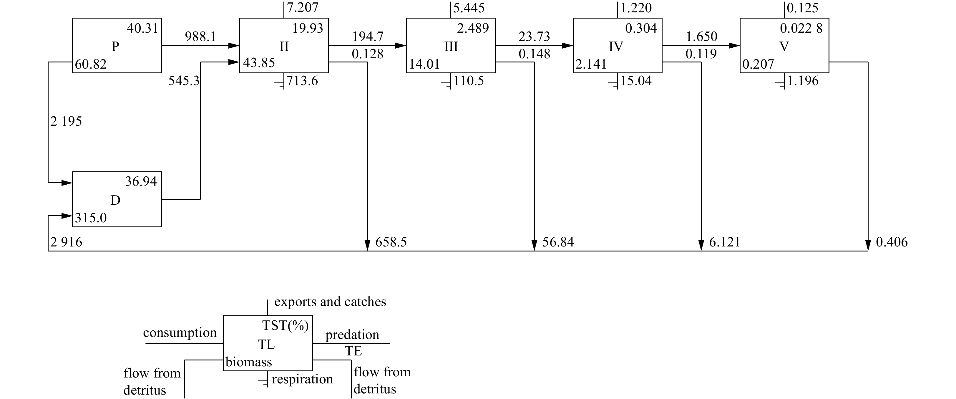
Figure 3. Lindeman spine representing of trophic flows from Qilianyu Islands coral reefs Ecopath model. P: primary producers; D: detritus; II–V: trophic levels; TST: total system throughput; TE: transfer efficiencies; TL: trophic level.
Figure 4. Qilianyu Islands coral reefs Ecopath model plot of functional group niche overlap. Point colors represent geometric mean of “prey overlap index” and “predator overlap index” (color scale to right); functional groups: 4, 7 small carnivorous and herbivorous fish; 14, 15 coral and zooplankton; 11, 13 other echinoderms and crustaceans.
Figure 5. Qilianyu Islands coral reefs model mixed trophic impact analysis. Positive (blue) and negative (red) values of mixed trophic impact index represent positive and negative effects, respectively. LCF, large carnivorous fish; MCF, medium carnivorous fish; SCF, small carnivorous fish; OF, omnivorous fish; CEF, coral-eating fish; HF, herbivorous fish; CTS, crown of thorns starfish; OE, other echinoderms; OM, other mollusca; SBI, small benthic invertebrates.
Figure 6. Keystone index for Qilianyu Islands coral reefs model functional groups. For each functional group, the keystone index (y-axis) is reported against their relative total impact on the trophic web (x-axis). Overall effects are relative to the maximum effect measured; the x-axis scale is between 0.0 and 1.0. The functional groups are ordered by decreasing keystone index; therefore, the key functional groups are those ranking among the first groups. Circles are proportional to the functional group biomass in the system.


 DownLoad:


 DownLoad: