Figure
1.
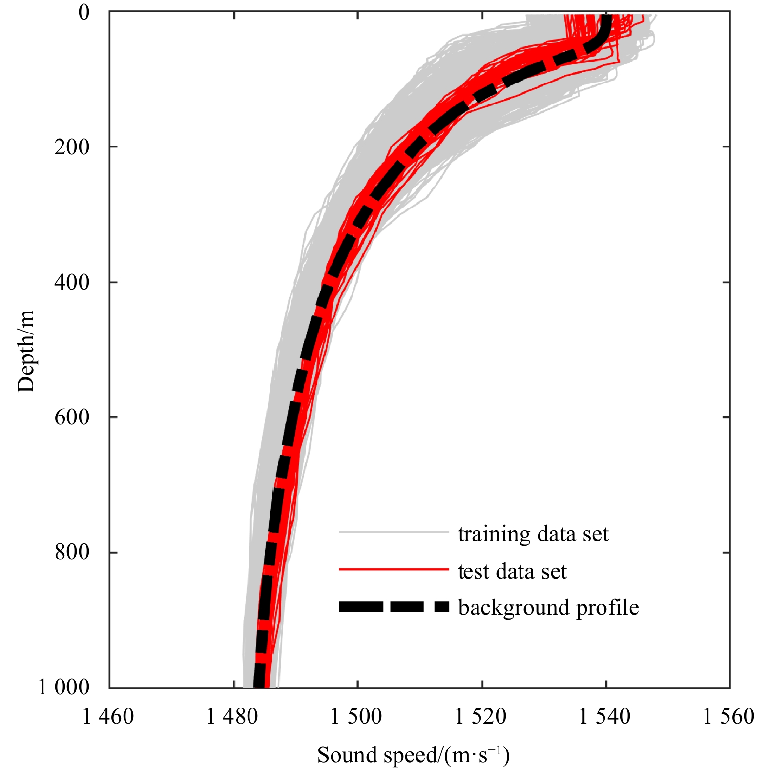
Sound speed profile samples and background profile.
| Citation: | Ke Qu, Binbin Zou, Jianbo Zhou. Rapid environmental assessment in the South China Sea: Improved inversion of sound speed profile using remote sensing data[J]. Acta Oceanologica Sinica, 2022, 41(7): 78-83. doi: 10.1007/s13131-022-2032-2

|
The core objective of rapid environmental assessment (REA) is to provide environmental nowcasts for operational activity in any arbitrary region of the global ocean. As a thorough understanding of variations in the sound speed profile (SSP) can help enhance the performance of sonar in civil and military applications, the rapid assessment of the SSP has become a focus of research in the area. However, as SSP measurement with broad spatiotemporal coverage is extremely time-consuming and laborious, it is almost impossible to obtain the 3D structure of the sound speed via in situ measurements. Although the water column is optically opaque, remote sensing is the only platform that can provide real-time observations of the ocean at a large scale. Therefore, it is feasible to obtain rapid assessments of the SSP using remote sensing data.
The thermal expansion and contraction of the water column, and conduction of heat on the surface of water form an intrinsic link between the parameters of the surface and profiles of the subsurface. Therefore, related research has focused on the sea level (SL) and the sea surface temperature (SST). Carnes confirmed the relationship between remote sensing data (SL and SST) and subsurface profiles in the Gulf Stream (Carnes et al., 1990), and then estimated the subsurface profiles of the Northwest Pacific and Northwest Atlantic Oceans by using single empirical orthogonal function regression (sEOF-r) (Carnes et al., 1994). As the empirical orthogonal function (EOF) and linear regression can significantly improve the efficiency of inversion, sEOF-r has been widely used in REA models, such as the US Navy’s forecasting system for the ocean (Fox et al., 2002). In the framework of sEOF-r, the vertical spatial and temporal characteristics of the oceanographic profile can be calculated by using remote sensing data in linear empirical relationships between the parameters of the surface and the subsurface (Meijers et al., 2011). A celebrated instance is that of the Modular Ocean Data Assimilation System (MODAS), which provides a dynamic climatology that can be used to obtain the height and temperature of the sea surface to predict underwater structures by constructing synthetic profiles generated by regression analysis (Rahaman et al., 2016). The SSP has also been reconstructed directly via sEOF-r (Chen et al., 2018).
In recent years, machine learning theory has been introduced to problems similar to the above. Since machine learning is a universal framework to solve for the inherent characteristics of the training set, nonlinear relationships between parameters of the surface and subsurface can be extracted without any assumption about the vertical structure of the water column. Hjelmervik used k-means clustering and gradient search to estimate real-time profiles from the surface parameters (Hjelmervik and Hjelmervik, 2013, 2014), and Chapman reconstructed subsurface velocities in the South Indian Ocean based on self-organizing maps (SOM) from the Archiving, Validation and Interpretation of Satellite Oceanographic data satellite product (Chapman and Charantonis, 2017). Compared with linear regression, machine learning has shown a better capability to reconstruct the subsurface profile (Bao et al., 2019; Su et al., 2019). However, one drawback of this method is the large amount of training data needed, where few samples of poor quality can significantly reduce its accuracy and reliability (Jain and Ali, 2006; Frederick et al., 2020).
Although the above method has been used in many parts of the world, the rapid assessment of the SSP has not been implemented in the South China Sea (SCS). The SCS is the largest marginal sea connecting the Indian Ocean and the Pacific Ocean. Its unique semi-closed basin structure, monsoon, exchange of water with the ocean, and other factors contribute to the complex distribution of its SSP, which poses a challenge to REA schemes. Compared with the other waters, samples from the SCS are sparse, and this makes it difficult to implement the relevant methods. This study used SSP inversion for the REA of the SCS. Challenges to the obtaining the REA of the SCS were examined, and a method of SSP inversion based on SOM was proposed. The SSPs in 2018 were estimated and compared with the results of sEOF-r. As the SCS had a complex mechanism of perturbations in its profile, the inversion of the SSP in this region can help develop better methods for REA.
Both sEOF-r and the SOM method were tested on the same training and validation datasets. The remote sensing data included the sea level anomalies (SLA) and sea surface temperature anomalies (SSTA), and Argo profiles were used to establish samples of the SSP.
The remote sensing data were obtained from the Copernicus Project (https://resources.marine.copernicus.eu). Both the SLA and SSTA were obtained from L4 satellite observation products with a temporal resolution of one day and spatial resolution of 0.25°.
All the Argo data were obtained from the Global Ocean Argo Scattering Data Collection (July 1997–June 2020) (Li et al., 2020), and were considered only if the depth of the sample from shallower than 5 m to deeper than 1 000 m. The SSPs were calculated via the empirical sound speed formula through the profiles of temperature and salinity (Del Grosso, 1974). Profiles in the range of 12°–20°N and 110°–120°E from 2009 to 2018 were selected to test inversion. A total of 1 679 profiles were obtained, ranging from 5 m to 1 000 m. As most variations were in the upper layers of the ocean, the depth-variable sampling rate proposed by the World Ocean Atlas 2018 was used. The training dataset consisted of all profiles in the SCS from 2009 to 2017, and 56 profiles from 2018 were used as the test set. The background profiles were the annual average data at a spatial resolution of 0.25° at the center of the clustering result of SCS class. Figure 1 shows all the SSPs. It is clear that the upper layers of the ocean featured a wide range of variation in sound speed. To analyze the reconstruction, the root mean-squared error (RMSE) was used to define the reconstruction error,
| $$ {\rm{RMSE}} = \sqrt {\frac{{\displaystyle\sum\limits_{d = 1}^{{\rm{DN}}} {\sum\limits_{s = 1}^{{\rm{SN}}} {{{(c_{d,s}^{\rm{m}} - c_{d,s}^{\rm{r}})}^2}} } }}{{{\rm{DN}} \times {\rm{SN}}}}} , $$ | (1) |
where
In the problem of SSP inversion, the sound speed profile
| $$ c(z,t) = {c_0}(z) + \sum\limits_{s = 1}^\infty {{a_s}(t){K_s}(z)} , $$ | (2) |
where
To analyze the difficulties of REA in the SCS, this study considered the classic sEOF-r as competing method. Based on a large number of historical observations, an approximately linear relationship was noted between the parameters of the surface and the projection coefficients. By taking advantage of the empirical relationships between SLA, SSTA, and coefficients of the EOF
| $$\begin{split} {a_s}(t) =& {A_{s,0}} + {A_{s,1}} \times {\rm{SLA}}(t) + {A_{s,2}}{\rm{SSTA}}(t) + \\ &{A_{s,3}}{\rm{SLA}}(t) \times {\rm{SSTA}}(t), {s = } 0,1,2, \cdots ,G , \end{split}$$ | (3) |
where
All methods of inversion are based on the assumption that modes of the EOF in the area of inversion at sea are consistent. In the ocean, 2°
Expanding the area of inversion can increase the number of samples, but the consistency of the EOF is difficult to guarantee in this case. Therefore, the consistency of modes of the EOF must be analyzed. In this paper, k-means clustering on the projection coefficients was used to check for the consistency of the modes of the EOF. By using the projection coefficients as the training set, the
| $$ b_s^m{\text{ = }}\frac{1}{{{N_m}}}\sum\limits_{n = 1}^N {{\text{δ} _{mn}}a_s^n} , $$ | (4) |
where
| $$ \sigma = \sqrt {\sum\limits_{n = 1}^N {\sum\limits_{m = 1}^M {{\text{δ} _{mn}}\sum\limits_{s = 1}^G {{{(a_s^n - b_s^m)}^2}} } } } . $$ | (5) |
The lowest deviations represent the lowest Euclidean distance, which is the best result of clustering. To solve the above, the fast k-means algorithm is used in 100 independent parallel runs to ensure that the global optimum is obtained.
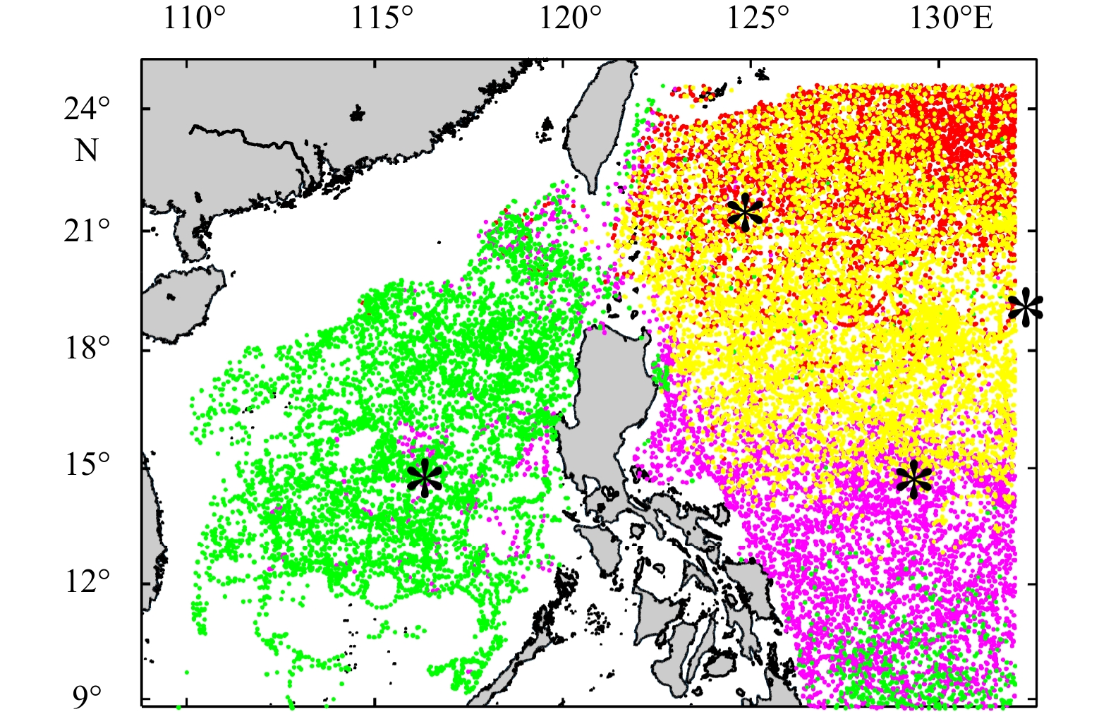
Figure 2 shows the consistency of EOFs in the SCS. To analyze their consistency, profiles from the Pacific Ocean were introduced, and a total of 27 620 profiles were finally obtained. The Argo samples from the SCS were concentrated in the basin, and almost all profiles belonged to the same class that was different from that of profiles of the Pacific Ocean. The results of clustering showed that samples from the SCS had a similar dynamic nature, where the center of the class could be used to approximate the background profile of all samples from the SCS. To deal with the problem of sparsity of the samples, all samples were statically analyzed in one grid cell. Modes of the EOF in the SCS exhibited spatial variation; if the samples were clustered in more classes, they scattered into different classes. Therefore, inversion errors increased with the expansion of the area of inversion.

Figure 3 shows the shapes of the first five modes of the EOF. According to the distribution of the amplitude of the EOF, the perturbation in sound speed mainly occurred in the range of depth of 200 m, and the amplitude was close to zero at around a depth of 1 000 m. We focused on reconstruction within 1 000 m. Table 1 gives properties of the reconstruction of the first five leading orders. The cumulative variance contribution of the first five modes was 96.7%. Although the SSP samples were recorded in a large area of the sea, a few leading modes of the EOF could still described most of the variations, and this confirmed the consistency of the EOF for the SCS. To identify the main modes of SSP perturbation while reducing noise, the first five orders of EOF were used in the subsequent comparison between the sEOF-r and the SOM method.
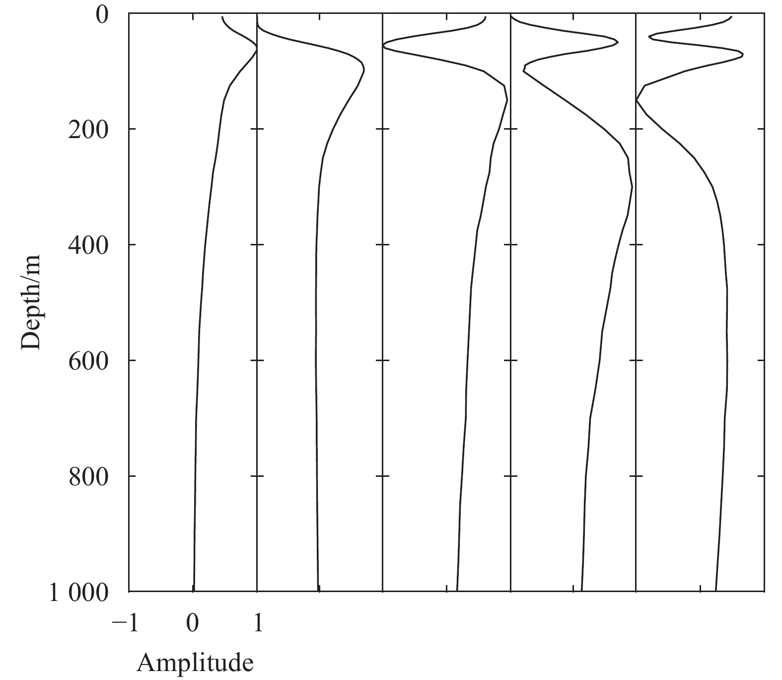
| EOF1 | EOF2 | EOF3 | EOF4 | EOF5 | |
| Variance contribution/% | 74.0 | 13.7 | 4.7 | 2.9 | 1.4 |
| Cumulative variance contribution/% | 74.0 | 87.7 | 92.4 | 95.3 | 96.7 |
| Reconstruction error/(m·s−1) | 2.00 | 1.38 | 1.09 | 0.85 | 0.72 |
 DownLoad:
CSV
DownLoad:
CSV
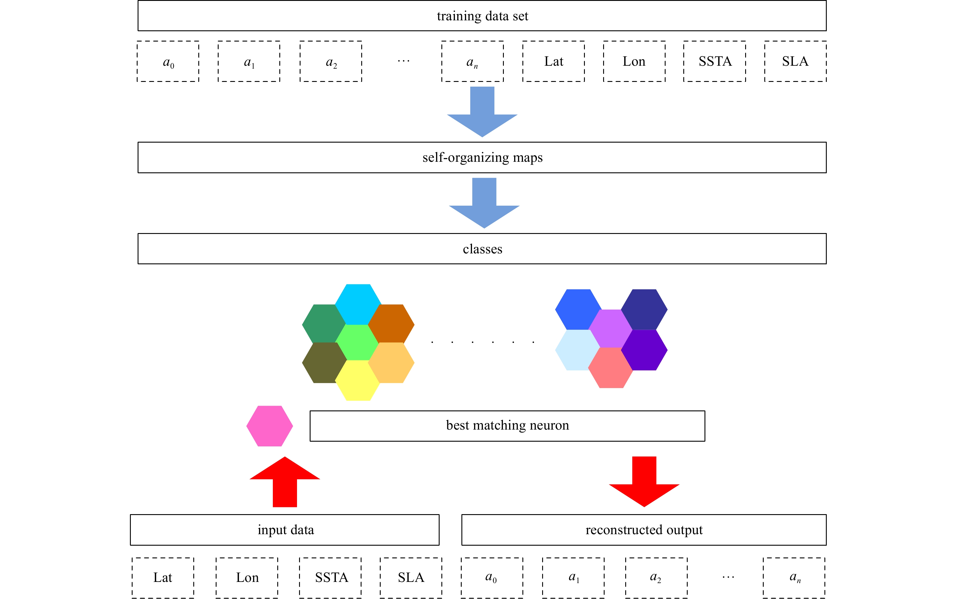
A flowchart of the proposed method is shown in Fig. 4. The SOM, which projects the training vectors into a topological structure on a 2D lattice by using competitive learning, is generally used to classify the data according to the similarity between them (Charantonis et al., 2015).

In the training phase, the projection coefficients of the EOF, SLA, SSTA, longitude, and latitude of the profile of one sample were entered as a training vector to train the map. Based on the SOM algorithm, all training vectors were assigned to different classes. Some reference vectors were also constructed between neighboring classes to form a 2D artificial neural network together with classes of the training vectors.
In the inversion phase, remote sensing data were entered into the neural map to identify the best-matching neuron. This neuron is defined as the neural unit with has the shortest Euclidian distance in the topological structure. As the distance only performed over the dimensions with available data, Chapman introduced a similarity function to calculate the truncated distance (Chapman and Charantonis, 2017):
| $$ d_E^p(x,{u^p}) = \sum\limits_{i \in {\rm{avail}}} {\left( {1 + \sum\limits_{j \in {\rm{missing}}} {{{({\rm{cor}}_{ij}^c)}^2}} } \right)} \times ({x_i} - u_i^p) , $$ | (6) |
where
Figure 5 shows a comparison of errors in the reconstruction of the SSP between sEOF-r and the SOM method. Except for a few samples, the accuracy of reconstruction of the SOM method was significantly higher than that of sEOF-r. The SSPs reconstructed by using the SOM had a mean error of 1.26 m/s, whereas this was 2.29 m/s for sEOF-r. The proposed method reduced the error by relieving the constraint of linear inversion and introducing a location-related parameter. In addition, the SOM method yielded more robust results. The maximum errors of the single SSP in the sEOF-r was 5.18 m/s, while the maximum errors in the SOM method was 2.19 m/s. Only about 18% (48%) of the estimated SSPs lay within an error limit of ±1.5 (±2) m/s. Because the linear regression model of the sEOF-r is based on the average feature of samples, the differences between individual characteristics and statistical feature has led to uncertainty in inversion using sEOF-r, especially in the SCS that featured a wide range of variation in sound speed. By eliminating the presupposed analytic expression, the SOM method greatly reduces the limitation of the simple linear regression. The total variance in the reconstruction error was 0.39 m/s using the SOM method, much lower than the 0.94 m/s obtained using sEOF-r. About 77% (93%) of the results lay within an error limit of ±1.5 (±2) m/s, which achieved major improvements over the linear regression. The SOM method described the complex relationship between parameters of the surface and profiles of the subsurface of each sample by using corresponding neurons on the topological map, which clearly improved the robustness of the results of inversion.

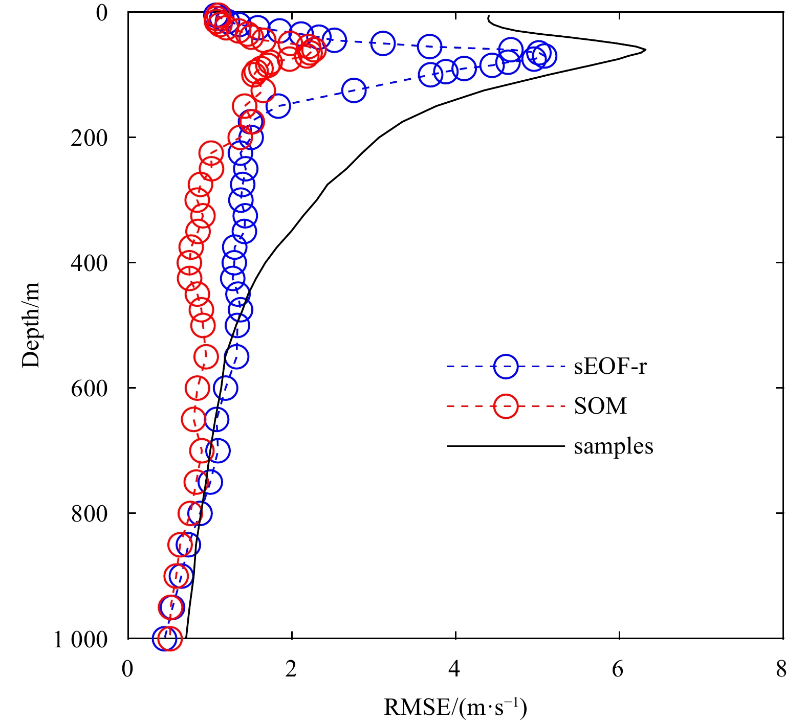
The errors of reconstruction at different depths are shown in Fig. 6. The RMSE of the SSP samples is 3.89 m/s with the maximum value of 6.26 m/s at 60 m. The SOM method performed effectively by reducing the mean error to 1.26 m/s and the maximum value to 2.26 m/s. The SSP estimated form the SOM method has an error of only about 0.15% as compared with the sound speed values. In addition, the error incurred by the SOM method was lower than that of the EOF method at almost all depths. As temperature was the dominant factor influencing the large variation in sound speed in the upper layers of the ocean, the large variations in SSP were observed owing to seasonal and diurnal variations in the mixed layer. We can infer that internal solitary waves and other dynamic marine activities also led to the concentration of error at these depths. Although the RMSE of the SSP samples was larger than 4 m/s in the surface layers, the reconstruction errors for both methods were also small. The accurate estimation near surface is because that the SSP near the surface is directly controlled and estimated by parameters of the sea surface. Similarly, the errors were less at deeper layer where the perturbations of sound speed were also less.

Figure 7 shows an example of the largest error in reconstruction using the SOM method. The maximum absolute error for the SOM method and the sEOF-r method were 3.55 m/s and 8.28 m/s, respectively, while the SOM method performed better at about two-thirds of the estimated depth. It is clear that the results of the SOM method still agreed better with the measured profile than those of sEOF-r. The main error in inversion still occurred due to error in the estimated depth of the mixed layer. As shown by the error between depths of 400 m and 800 m, perturbations in the sound speed caused by turbulence or water mass were difficult to describe. Because the daily average of the sea surface temperature was used, short-term perturbations were difficult to represent based on the inversion of the parameters of remote sensing.
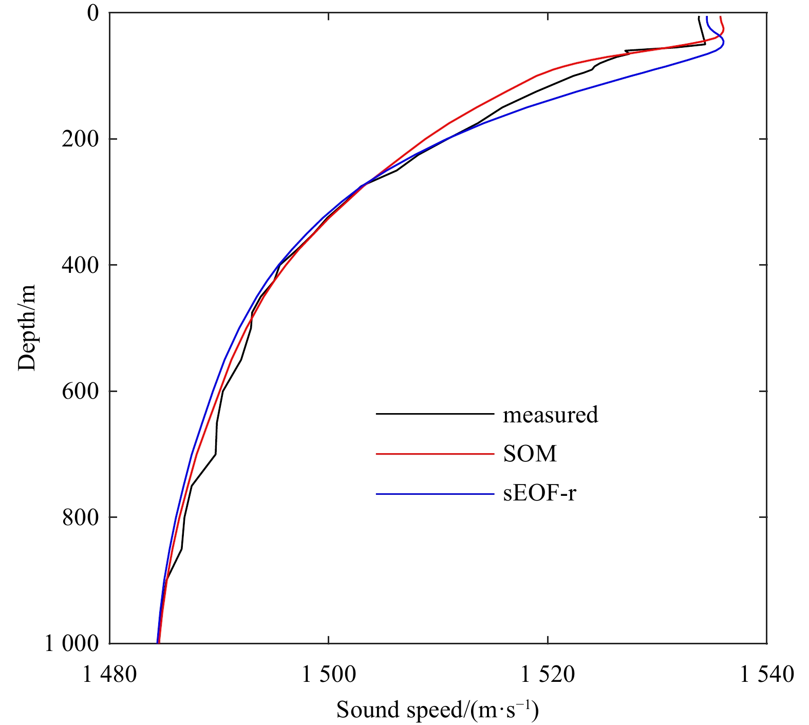
Figure 8 shows a comparison between the measured and the estimated values of the first five projection coefficients. It is clear that the SOM method delivered close to perfect results. The sEOF-r method significantly deviated from the reference line. For the first five orders, the Pearson correlation coefficients of the measured projection coefficients and the inversion results of the SOM (sEOF-r) method were 0.91 (0.25), 0.78 (0.73), 0.83 (0.24), 0.89 (0.70) and 0.86 (0.46), respectively. With an increase in order, the error in the projection coefficient tended to increase. In light of the contribution of the reconstructed mode of the EOF to the variance and errors in inversion, five orders of inversion were sufficient to ensure the accuracy of reconstruction without incurring a large error in case of the SCS.

Based on k-means clustering, this study showed that the EOFs of the SSP of the SCS were consistent. The problem of too few samples to determine the REA of the SCS was solved by expanding the area of inversion to the entire SCS. However, due to the complexity of and spatial differences in perturbations of the SSP, the classical sEOF-r method could not be used to accurately calculate the SSP.
A machine learning method based on the SOM was proposed and verified here. We used the topology of neurons for the rapid assessment of the SSP. For all samples of SSP from the South China Sea in 2018, the average reconstruction error was 1.26 m/s, only half of that incurred by sEOF-r. The maximum error in SSP inversion occurred at a depth of around 100 m, and was likely caused by large variations in the mixing layer. As the neuronal topology of the SOM method can accommodate more parameters, for instance, net radiation and wind speed, this can help further reduce the error caused by fluctuations in the mixing layer. Moreover, to solve the problem of sparse samples for the SCS, further work is needed to introduce physical mechanisms to ensure the accuracy and robustness of its REA.
| [1] |
Bao Senliang, Zhang Ren, Wang Huizan, et al. 2019. Salinity profile estimation in the Pacific Ocean from satellite surface salinity observations. Journal of Atmospheric and Oceanic Technology, 36(1): 53–68. doi: 10.1175/JTECH-D-17-0226.1
|
| [2] |
Bianco M J, Gerstoft P. 2017. Dictionary learning of sound speed profiles. The Journal of the Acoustical Society of America, 141(3): 1749–1758. doi: 10.1121/1.4977926
|
| [3] |
Carnes M R, Mitchell J L, de Witt P W. 1990. Synthetic temperature profiles derived from Geosat altimetry: Comparison with air-dropped expendable bathythermograph profiles. Journal of Geophysical Research, 95(C10): 17979–17992. doi: 10.1029/JC095iC10p17979
|
| [4] |
Carnes M R, Teague W J, Mitchell J L. 1994. Inference of subsurface thermohaline structure from fields measurable by satellite. Journal of Atmospheric and Oceanic Technology, 11(2): 551–566. doi: 10.1175/1520-0426(1994)011<0551:IOSTSF>2.0.CO;2
|
| [5] |
Chapman C, Charantonis A A. 2017. Reconstruction of subsurface velocities from satellite observations using iterative self-organizing maps. IEEE Geoscience and Remote Sensing Letters, 14(5): 617–620. doi: 10.1109/LGRS.2017.2665603
|
| [6] |
Charantonis A A, Testor P, Mortier l, et al. 2015. Completion of a sparse GLIDER database using multi-iterative Self-Organizing Maps (ITCOMP SOM). Procedia Computer Science, 51: 2198–2206. doi: 10.1016/j.procs.2015.05.496
|
| [7] |
Chen Cheng, Ma Yuanliang, Liu Ying. 2018. Reconstructing sound speed profiles worldwide with sea surface data. Applied Ocean Research, 77: 26–33. doi: 10.1016/j.apor.2018.05.002
|
| [8] |
Del Grosso V A. 1974. New equation for the speed of sound in natural waters (with comparisons to other equations). The Journal of the Acoustical Society of America, 56(4): 1084–1091. doi: 10.1121/1.1903388
|
| [9] |
Fox D N, Teague W J, Barron C N, et al. 2002. The modular ocean data assimilation system (MODAS). Journal of Atmospheric and Oceanic Technology, 19(2): 240–252. doi: 10.1175/1520-0426(2002)019<0240:TMODAS>2.0.CO;2
|
| [10] |
Frederick C, Villar S, Michalopoulou Z H. 2020. Seabed classification using physics-based modeling and machine learning. The Journal of the Acoustical Society of America, 148(2): 859–872. doi: 10.1121/10.0001728
|
| [11] |
Hjelmervik K T, Hjelmervik K. 2013. Estimating temperature and salinity profiles using empirical orthogonal functions and clustering on historical measurements. Ocean Dynamics, 63(7): 809–821. doi: 10.1007/s10236-013-0623-3
|
| [12] |
Hjelmervik K, Hjelmervik K T. 2014. Time-calibrated estimates of oceanographic profiles using empirical orthogonal functions and clustering. Ocean Dynamics, 64(5): 655–665. doi: 10.1007/s10236-014-0704-y
|
| [13] |
Jain S, Ali M M. 2006. Estimation of sound speed profiles using artificial neural networks. IEEE Geoscience and Remote Sensing Letters, 3(4): 467–470. doi: 10.1109/LGRS.2006.876221
|
| [14] |
LeBlanc L R, Middleton F H. 1980. An underwater acoustic sound velocity data model. The Journal of the Acoustical Society of America, 67(6): 2055–2062. doi: 10.1121/1.384448
|
| [15] |
Li Zhaoqin, Liu Zenghong, Lu Shaolei. 2020. Global Argo data fast receiving and post-quality-control system. IOP Conference Series: Earth and Environmental Science, 502: 012012. doi: 10.1088/1755-1315/502/1/012012
|
| [16] |
Meijers A J S, Bindoff N L, Rintoul S R. 2011. Estimating the four-dimensional structure of the Southern Ocean using satellite altimetry. Journal of Atmospheric and Oceanic Technology, 28(4): 548–568. doi: 10.1175/2010JTECHO790.1
|
| [17] |
Rahaman H, Behringer B W, Penny S G, et al. 2016. Impact of an upgraded model in the NCEP Global Ocean Data Assimilation System: The tropical Indian Ocean. Journal of Geophysical Research: Oceans, 121(11): 8039–8062. doi: 10.1002/2016JC012056
|
| [18] |
Su Hua, Yang Xin, Lu Wenfang, et al. 2019. Estimating subsurface thermohaline structure of the global ocean using surface remote sensing observations. Remote Sensing, 11(13): 1598. doi: 10.3390/rs11131598
|
| 1. | Guojun Xu, Ke Qu, Zhanglong Li, et al. Enhanced Inversion of Sound Speed Profile Based on a Physics-Inspired Self-Organizing Map. Remote Sensing, 2025, 17(1): 132. doi:10.3390/rs17010132 | |
| 2. | Marzieh Mokarram, Tam Minh Pham. Environmental Monitoring of Oil Pollution in the Marine Waters using Machine Learning and Remote Sensing. Advances in Space Research, 2025. doi:10.1016/j.asr.2025.01.062 | |
| 3. | Yuyao Liu, Yu Chen, Zhou Meng, et al. Performance of single empirical orthogonal function regression method in global sound speed profile inversion and sound field prediction. Applied Ocean Research, 2023, 136: 103598. doi:10.1016/j.apor.2023.103598 | |
| 4. | Xilu Qian. Research on the coordinated development model of marine ecological environment protection and economic sustainable development. Journal of Sea Research, 2023, 193: 102377. doi:10.1016/j.seares.2023.102377 |


Figures(8) / Tables(1)

Supported by:
Beijing Renhe Information Technology Co. Ltd

Ke Qu, Binbin Zou, Jianbo Zhou. Rapid environmental assessment in the South China Sea: Improved inversion of sound speed profile using remote sensing data[J]. Acta Oceanologica Sinica, 2022, 41(7): 78-83. doi: 10.1007/s13131-022-2032-2

| EOF1 | EOF2 | EOF3 | EOF4 | EOF5 | |
| Variance contribution/% | 74.0 | 13.7 | 4.7 | 2.9 | 1.4 |
| Cumulative variance contribution/% | 74.0 | 87.7 | 92.4 | 95.3 | 96.7 |
| Reconstruction error/(m·s−1) | 2.00 | 1.38 | 1.09 | 0.85 | 0.72 |
DownLoad:
CSV
 DownLoad:


 DownLoad: