

Figure
1.
Typical SAR ISW Images obtained from Sentinel-1 (a–c) and GF-3 (d–f).
| Citation: | Zhi Ding, Fenzhen Su, Yanan Chen, Ying Liu, Xue Feng, Wenqiu Hu, Fengqin Yan, He Li, Pujia Yu, Xuguang Tang. Whether human-induced activities could change the gradient pattern of coastal land use along the sea-land direction: a case study in Manila Bay, Philippines[J]. Acta Oceanologica Sinica, 2023, 42(2): 163-174. doi: 10.1007/s13131-022-2026-0

|
The Malacca Strait with 1 080 km long is the most important energy transport route. Due that the internal solitary waves (ISWs) have great influence on the navigation of ships and submarines, especially, Malacca Strait is the area where the ISWs occur frequently, it is necessary to study the characteristics of the ISWs in Malacca Strait.
It is well known that ISWs phenomenon shows strong randomness, and its amplitude, propagation velocity and wavelength are greatly affected by hydrology and other external environment (Fang and Du, 2005; Li et al., 2013; Alford et al., 2010; Cai and Xie, 2010; Huang et al., 2007; Hyder et al., 2005; Lai et al., 2010). The research of ISWs based on SAR image usually includes the following two aspects. One is to study the temporal and spatial distribution of ISWs. For example, in 2000, Hsu et al. (2000) studied the distribution of ISWs in the South China Sea based on 5-year satellite remote sensing images. Using satellite SAR data from July to October 2007, Kozlov et al. (2015) studied the characteristics of short-period ISWs in the Kara Sea. Filonov et al. (2014) studied the spatial distribution of ISWs of Todos Santos by means of the combination of real measurement and remote sensing. Another one is the imaging mechanism of ISWs on SAR image and the inversion of ISWs parameters. For example, in 2013, Liu et al. (2013) calculated the nonlinear phase velocity of the ISWs in the South China Sea using multi-source remote sensing data, and found that the velocity of the ISWs was greatly affected by the depth of water. In 2016, combined with nonlinear Schrodinger (NLS) equation, our team obtained the inversion model of SAR ISWs parameters, and the inversion results are close to the measured data (Zhang et al., 2016). With the increasing number of satellites in orbit, the understanding of ISWs by multi-source remote sensing becomes to be more and more comprehensive (Jackson, 2007; Schuler et al., 2003).
In a word, there is no research on the ISWs in Malacca Strait up to date. In this paper, ISWs in Malacca Strait are investigated from the spatial distribution of the waves, the velocity and amplitude of the ISWs, and so on, which will provide valuable scientific references for maritime navigation and marine engineering.
The Malacca Strait is located in the region of 0°–6°N and 97°–104°E. In order to observe and analyze the characteristics of ISWs in the Malacca Strait, Sentinel-1 SAR data from June 2015 to December 2016 and GF-3 data from April 2018 to March 2019 are collected. Because of the limitation of SAR orbital period, we obtain 20 Sentinel-1 images and 24 GF-3 images in total, and 344 ISW packets and ISWs are collected.
It can be seen from Fig. 1 that the ISWs in the Malacca Strait mainly appear in the form of wave packets and single solitary waves. Though the direction of ISWs propagation seems to be very complex, however, it always tends to propagate towards the shore.
Furtherly, according to the position and the crest length of the leading wave in the ISW packets in 45 SAR images, the spatial distribution of the wave and the length distribution of the leading wave crest in the Malacca Strait are obtained, which are shown in Fig. 2 and Fig. 3, respectively. As shown in Fig. 2, in region A, the depth of water in this area is about 50–100 m, and the largest wave packets is observed, accompany with a relatively long crest length of the leading wave. In the middle of the Malacca Strait (region B), the water depth is about 20–50 m, the ISW propagates in the form of wave packets and single solitary waves, and the crest length of the leading wave becomes shorter. In the southeast of the Malacca Strait (region C), the water depth is relatively shallow, with the shallowest part of only 4 m, and the ISW is mostly in the form of wave packets and single solitary waves, with the shortest crest length of the leading wave, but it is noticing that the ISWs is broken seriously, and the direction of the ISWs is also relatively messy.


By observed from satellite images, it can be found that there are three to seven ISWs on average in the Malacca Strait, with a maximum of 12 ISWs. The maximum (minimum) crest length of the wave packet is about 39 km (1.5 km) in the Fig. 2, and the crest length of the leading wave becomes to be shorter and shorter towards the southeast. Totally, 344 crest length of the leading wave are observed, in which 35 lines are more than 20 km in length, and most of them are located in the northwest region. In addition, most crest length of the leading wave less than 20 km are located in the regions B and C, and the number of crest length of the leading wave from 4 km to 14 km is about 273 crest lines, which accounts for the vast majority of total lines.
In addition, the occurrence of ISWs has a great relationship with seasons. Figure 4 shows the distribution of ISWs in different seasons. The largest number of ISWs observed from remote sensing images occurred from January to march, and the smallest from October to December. Most of the ISWs observed in SAR images from April to September occurred in region C.

The inversion of the ISWs parameters greatly depends on the two layer stratification. Temperature, salt and density data of the studied area are selected from the annual average data of World Ocean Atlas (2013), and hierarchical information is obtained by calculating the vertical distribution. The calculated temperature, salinity, density and buoyancy frequency curve are showed in Fig. 5. The water depth corresponding to the inflection point of buoyancy frequency in Fig. 5d is the upper water depth, about 25 m. The density corresponding to the upper water depth is found in the density curve, and the upper and lower average densities are calculated as 1 019.9 kg/m3 and 1 020.9 kg/m3 respectively.

Because of the balance between nonlinear effect and dispersion effect, the ISWs can be stable and spread over long distance.
The ISWs propagation equation adopts NLS equation. Combined with the SAR imaging mechanism of the ISWs, the amplitude inversion model of the ISWs based on the SAR image is established (NLS equation) (Zhang et al., 2016).
| $$\left\{ \begin{split} & D = 1.76l,\qquad \alpha \beta > 0\\ & D = 1.32l,\qquad \alpha \beta < 0 \end{split} \right.,$$ | (1) |
| $$\left\{ \begin{split} & {A_0} = \frac{{1.76}}{D}\sqrt {\left| {\frac{{2\alpha }}{\beta }} \right|},\qquad \alpha \beta > 0\\ & {A_0} = \frac{{1.32}}{D}\sqrt {\left| {\frac{{2\alpha }}{\beta }} \right|},\qquad \alpha \beta < 0 \end{split} \right.,$$ | (2) |
where A0 is the amplitude of the ISWs,
Then we apply the NLS amplitude inversion model to the previous 45 SAR images, and extract the distance D between the brightest spot and the darkest spot and hydrological parameters from each SAR image. The amplitude A0 of ISWs can be obtained from Eq. (2). We calculate the amplitude of ISWs happened in the Malacca Strait with water depth greater than 30 m.
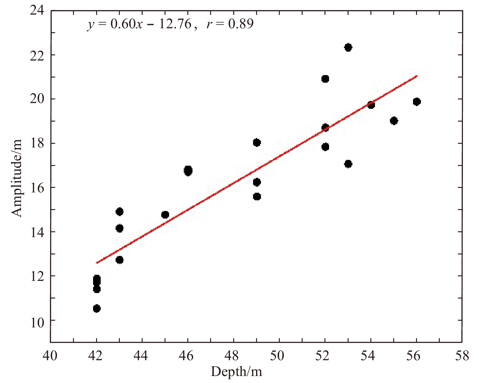
By extracting the characteristic parameters of ISWs in the Malacca Strait, the amplitude distribution is obtained, as shown in Fig. 6. In region A, the maximum amplitude obtained by NLS amplitude inversion model is 23.9 m, which is located at the water depth of 78 m, and the average amplitude of ISWs in this area is about 18.4 m. The maximum amplitude in region B calculated by NLS amplitude inversion model is 17.9 m, the minimum amplitude is 4.7 m, and the average amplitude of ISWs is about 10.9 m. The water depth in region C is shallow. The maximum and minimum amplitude calculated by NLS amplitude inversion model are 14.1 m and 4.7 m respectively, and the average amplitude is 9.6 m. In addition, we also analyze the amplitude of the one ISW. Figure 7 is a SAR image from March 14, 2016, we extracted the parameter and calculated the amplitude of ISWs. Each red dot in Fig. 7 is the extraction position of the ISWs parameter, combined with the local depth of water, the relationship between amplitude and depth of water is shown in Fig. 8. From Fig. 8, it can be found that even in the same ISW, the amplitude of ISWs is different, and the amplitude distribution is linearly related to the water depth. Figures 4 and 8 show that in Malacca Strait, with the decrease of water depth, the amplitude decreases. This may be due to the increase of the nonlinear effect of ISWs with the shallow water depth, which leads to the breakage of ISWs.

ISWs in the Malacca Strait can be divided into two types: single solitary waves and solitary wave packets. Therefore, we use NLS equation to derive the group velocity of solitary wave packets and KdV equation to obtain the phase velocity of single solitary waves.
The group velocity formula derived from the NLS equation (Zhang et al., 2015) is
| $${c_g} = \frac{{\rm d\omega }}{{\rm dk}} = \frac{\omega }{{2k}}\left[ {1 + \frac{{2k{h_2}}}{{ {\rm {sh}}(2k{h_2})}}} \right] ,$$ | (3) |
where k is the wave number, h2 is the depth of the lower layer, and
The phase velocity formula obtained by KdV equation (Zheng et al., 2001) is
| $$c = {\left[ {\frac{{g({\rho _2} - {\rho _1}){h_1}{h_2}}}{{{\rho _2}{h_1} + {\rho _1}{h_2}}}} \right]^{1/2}} + \frac{{\alpha {A_0}}}{3}, $$ | (4) |
where hl and h2 are the thickness of the upper and lower layers, respectively, and their water densities are
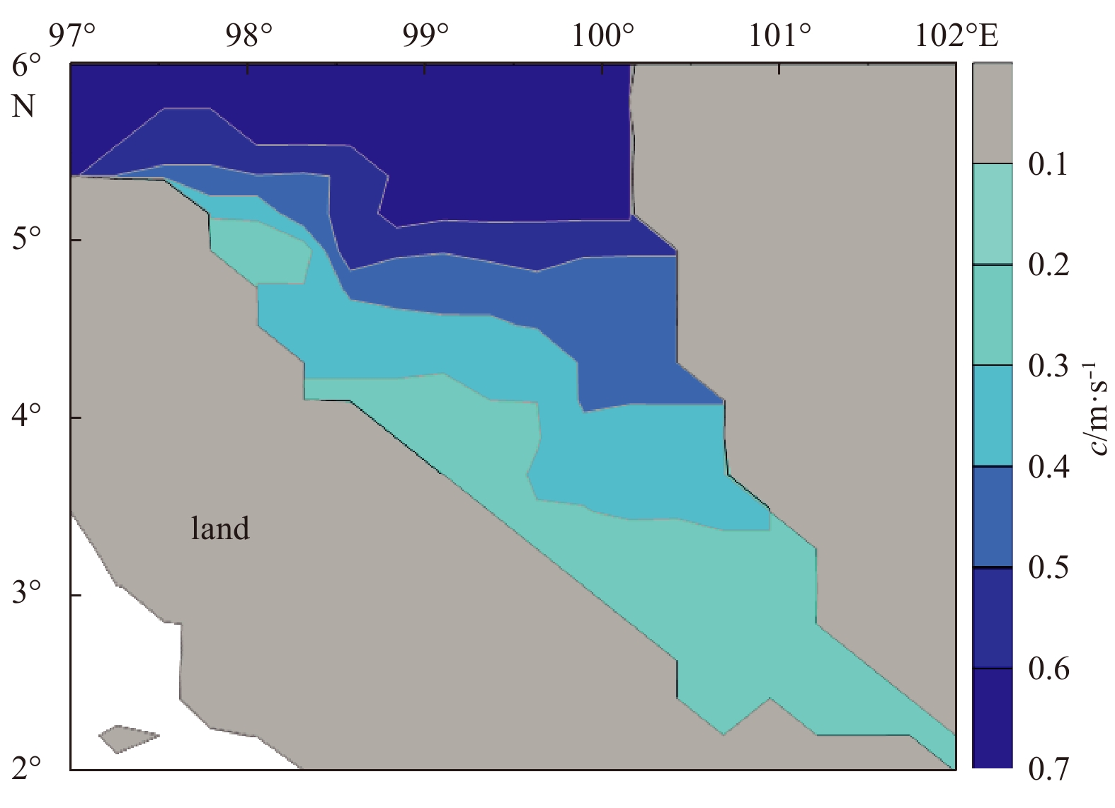
The propagation velocity of ISWs is affected by many factors, such as water depth, stratification. The two-dimensional water depth distribution map of Malacca Strait has been given in Fig. 2. It can be seen that the depth of the water in the south is the shallower, and the deeper is to the northwest. The distribution characteristics of the group velocity and the phase velocity in Malacca Strait are analyzed. Figure 9 shows the group velocity distribution of ISWs in Malacca Strait calculated by using the group velocity formula derived from the NLS equation. Figure 10 shows the distribution of phase velocity calculated by KdV equation.

As can be seen from Fig. 9, the group velocity of the wave packets reduced from 0.4 m/s to 0.12 m/s and the phase velocity of ISWs in Fig. 10 decreases from 0.6 m/s to 0.26 m/s. In general, the group velocity and phase velocity of ISWs in Malacca Strait are related to the topography.

Based on the Sentinel-1 and GF-3 SAR data, totally 45 SAR images in Malacca Strait are obtained, and the characteristic parameters of the ISWs in Malacca Strait are studied. The distribution of ISWs and crest length of the leading waves in Malacca Strait are statistically analyzed. It is found that ISWs are present in most of Malacca Strait, and the ISWs appear in the form of wave packets and single solitary waves. Furthermore, the direction of ISWs propagation is more complex, but the ISWs always tends to propagate towards the shore. The crest length of the leading wave is the longest in the northwest.
In addition, the group velocity and amplitude distributions of the area are calculated based on the high-order completely NLS equation inversion model. The phase velocity is obtained by KdV equation. The group velocity and phase velocity of ISWs are closely related to water depth and stratification. From northwest to southeast, with the water depth becoming shallow, the group velocity and phase velocity of ISWs becomes smaller. The group velocity distribution is between 0.12 m/s and 0.40 m/s, the phase velocity distribution is between 0.26 m/s and 0.6 m/s, and the amplitude of the ISWs is in the range of 4.7–23.9 m. The general trend of the amplitude and velocity is decreasing, which indicates that with the depth of water decreases, the nonlinearity increases, leading to the breakup of ISWs.
|
Ai Bin, Ma Chunlei, Zhao Jun, et al. 2020. The impact of rapid urban expansion on coastal mangroves: a case study in Guangdong Province, China. Frontiers of Earth Science, 14: 37–49. doi: 10.1007/s11707-019-0768-6
|
|
Al Abid F B. 2014. A novel approach for PAM clustering method. International Journal of Computer Applications, 86(17): 1–5. doi: 10.5120/15074-3039
|
|
Bindra K, Mishra A, Suryakant. 2019. Effective data clustering algorithms. In: Ray K, Sharma T K, Rawat S, et al., eds. Soft Computing: Theories and Applications. Singapore: Springer, 419–432
|
|
Cárdenas J A R, Torres G P. 2021. Geospatial data mining techniques survey. In: Oliva D, Houssein E H, Hinojosa S, eds. Metaheuristics in Machine Learning: Theory and Applications. Cham: Springer, 635–643
|
|
Chen Yewang, Hu Xiaoliang, Fan Wentao, et al. 2020. Fast density peak clustering for large scale data based on kNN. Knowledge-Based Systems, 187: 104824. doi: 10.1016/j.knosys.2019.06.032
|
|
Dado J M, Narisma G T. 2022. The effect of urban expansion in Metro Manila on the southwest monsoon rainfall. Asia-Pacific Journal of Atmospheric Sciences, 58(1): 1–12. doi: 10.1007/s13143-019-00140-x
|
|
Di Xianghong, Hou Xiyong, Wang Yuandong, et al. 2015. Spatial-temporal characteristics of land use intensity of coastal zone in China during 2000–2010. Chinese Geographical Science, 25(1): 51–61. doi: 10.1007/s11769-014-0707-0
|
|
Ding Zhi, Liao Xiaohan, Su Fenzhen, et al. 2017. Mining coastal land use sequential pattern and its land use associations based on association rule mining. Remote Sensing, 9(2): 116. doi: 10.3390/rs9020116
|
|
Ding Zhi, Su Fenzhen, Zhang Junjue, et al. 2019. Clustering coastal land use sequence patterns along the sea–land direction: a case study in the coastal zone of Bohai Bay and the Yellow River Delta, China. Remote Sensing, 11(17): 2024. doi: 10.3390/rs11172024
|
|
Disegna M, D’Urso P, Durante F. 2017. Copula-based fuzzy clustering of spatial time series. Spatial Statistics, 21: 209–225. doi: 10.1016/j.spasta.2017.07.002
|
|
Du Mingjing, Ding Shifei, Jia Hongjie. 2016. Study on density peaks clustering based on k-nearest neighbors and principal component analysis. Knowledge-Based Systems, 99: 135–145. doi: 10.1016/j.knosys.2016.02.001
|
|
Feng Yu, Sun Tao, Zhu Meisha, et al. 2018. Salt marsh vegetation distribution patterns along groundwater table and salinity gradients in Yellow River Estuary under the influence of land reclamation. Ecological Indicators, 92: 82–90. doi: 10.1016/j.ecolind.2017.09.027
|
|
Garcia K B, Malabrigo Jr P L, Gevaña D T. 2014. Philippines’ mangrove ecosystem: status, threats and conservation. In: Faridah-Hanum I, Latiff A, Hakeem K R, et al., eds. Mangrove Ecosystems of Asia. New York: Springer, 81–94
|
|
Grachev A A, Leo L S, Fernando H J S, et al. 2018. Air–sea/land interaction in the coastal zone. Boundary-Layer Meteorology, 167(2): 181–210. doi: 10.1007/s10546-017-0326-2
|
|
Hadley D. 2009. Land use and the coastal zone. Land Use Policy, 26 (Suppl 1): S198–S203
|
|
Hahus I, Migliaccio K, Douglas-Mankin K, et al. 2018. Using cluster analysis to compartmentalize a large managed wetland based on physical, biological, and climatic geospatial attributes. Environmental Management, 62(3): 571–583. doi: 10.1007/s00267-018-1050-5
|
|
Hirschberg D S. 1977. Algorithms for the longest common subsequence problem. Journal of the ACM, 24(4): 664–675. doi: 10.1145/322033.322044
|
|
Hou Xiyong, Xu Xinliang. 2011. Spatial patterns of land use in coastal zones of China in the early 21st century. Geographical Research (in Chinese), 30(8): 1370–1379
|
|
Hu Luojia, Li Wenyu, Xu Bing. 2018. Monitoring mangrove forest change in China from 1990 to 2015 using Landsat-derived spectral-temporal variability metrics. International Journal of Applied Earth Observation and Geoinformation, 73: 88–98. doi: 10.1016/j.jag.2018.04.001
|
|
Hu Wenjia, Wang Yuyu, Zhang Dian, et al. 2020. Mapping the potential of mangrove forest restoration based on species distribution models: A case study in China. Science of The Total Environment, 748: 142321. doi: 10.1016/j.scitotenv.2020.142321
|
|
Huang Baoying, Li Zhijian, Dong Chengcheng, et al. 2021. The effects of urbanization on vegetation conditions in coastal zone of China. Progress in Physical Geography: Earth and Environment, 45(4): 564–579. doi: 10.1177/0309133320979501
|
|
Huang Chong, Zhang Chenchen, Liu Qingsheng, et al. 2020. Land reclamation and risk assessment in the coastal zone of China from 2000 to 2010. Regional Studies in Marine Science, 39: 101422. doi: 10.1016/j.rsma.2020.101422
|
|
Islam M M, Shamsuddoha M. 2018. Coastal and marine conservation strategy for Bangladesh in the context of achieving blue growth and sustainable development goals (SDGs). Environmental Science & Policy, 87: 45–54
|
|
Kumar P, Wasan S K. 2011. Comparative study of k-means, pam and rough k-means algorithms using cancer datasets. In: Proceedings of CSIT: 2009 International Symposium on Computing, Communication, and Control (ISCCC 2009). Singapore: IACSIT Press, 136–140
|
|
Li Huiying, Man Weidong, Li Xiaoyan, et al. 2017. Remote sensing investigation of anthropogenic land cover expansion in the low-elevation coastal zone of Liaoning Province, China. Ocean & Coastal Management, 148: 245–259
|
|
Li Qian, Yu Yang, Jiang Xiaoqian, et al. 2019. Multifactor-based environmental risk assessment for sustainable land-use planning in Shenzhen, China. Science of The Total Environment, 657: 1051–1063. doi: 10.1016/j.scitotenv.2018.12.118
|
|
Li Yuan, Zhang Haibo, Li Qingbo, et al. 2016. Characteristics of residual organochlorine pesticides in soils under different land-use types on a coastal plain of the Yellow River Delta. Environmental Geochemistry and Health, 38(2): 535–547. doi: 10.1007/s10653-015-9738-4
|
|
Liu Yubin, Hou Xiyong, Li Xiaowei, et al. 2020. Assessing and predicting changes in ecosystem service values based on land use/cover change in the Bohai Rim coastal zone. Ecological Indicators, 111: 106004. doi: 10.1016/j.ecolind.2019.106004
|
|
Marani M, Da Lio C, D’Alpaos A. 2013. Vegetation engineers marsh morphology through multiple competing stable states. Proceedings of the National Academy of Sciences of the United States of America, 110(9): 3259–3263. doi: 10.1073/pnas.1218327110
|
|
Martinez M L, Silva R, Lithgow D, et al. 2017. Human impact on coastal resilience along the coast of Veracruz, Mexico. Journal of Coastal Research, 77(sp1): 143–153
|
|
Mialhe F, Gunnell Y, Mering C, et al. 2016. The development of aquaculture on the northern coast of Manila Bay (Philippines): an analysis of long-term land-use changes and their causes. Journal of Land Use Science, 11(2): 236–256. doi: 10.1080/1747423X.2015.1057245
|
|
Mishra B K, Mebeelo K, Chakraborty S, et al. 2021. Implications of urban expansion on land use and land cover: towards sustainable development of Mega Manila, Philippines. GeoJournal, 86(2): 927–942. doi: 10.1007/s10708-019-10105-2
|
|
Moschetto F A, Ribeiro R B, De Freitas D M. 2021. Urban expansion, regeneration and socioenvironmental vulnerability in a mangrove ecosystem at the southeast coastal of São Paulo, Brazil. Ocean & Coastal Management, 200: 105418
|
|
Nor A N M, Corstanje R, Harris J A, et al. 2017. Impact of rapid urban expansion on green space structure. Ecological Indicators, 81: 274–284. doi: 10.1016/j.ecolind.2017.05.031
|
|
Politi E, Paterson S K, Scarrott R, et al. 2019. Earth observation applications for coastal sustainability: potential and challenges for implementation. Anthropocene Coasts, 2(1): 306–329. doi: 10.1139/anc-2018-0015
|
|
Ray G C. 1991. Coastal-zone biodiversity patterns. BioScience, 41(7): 490–498. doi: 10.2307/1311807
|
|
Ray G C, Hayden B P. 1992. Coastal zone ecotones. In: Hansen A J, Castri F, eds. Landscape Boundaries. New York: Springer, 403–420
|
|
Rodriguez A, Laio A. 2014. Clustering by fast search and find of density peaks. Science, 344(6191): 1492–1496. doi: 10.1126/science.1242072
|
|
Sajjad M, Li Yangfan, Tang Zhenghong, et al. 2018. Assessing hazard vulnerability, habitat conservation, and restoration for the enhancement of mainland China’s coastal resilience. Earth’s Future, 6(3): 326–338. doi: 10.1002/2017EF000676
|
|
Sheik M, Chandrasekar N. 2011. A shoreline change analysis along the coast between Kanyakumari and Tuticorin, India, using digital shoreline analysis system. Geo-spatial Information Science, 14(4): 282–293. doi: 10.1007/s11806-011-0551-7
|
|
Shi Lifeng, Liu Fang, Zhang Zengxiang, et al. 2015. Spatial differences of coastal urban expansion in China from 1970s to 2013. Chinese Geographical Science, 25(4): 389–403. doi: 10.1007/s11769-015-0765-y
|
|
Tseng Kuo-Tseng, Chan De-Sheng, Yang Chang-Biau, et al. 2018. Efficient merged longest common subsequence algorithms for similar sequences. Theoretical Computer Science, 708: 75–90. doi: 10.1016/j.tcs.2017.10.027
|
|
Vallejo Jr B M, Aloy A B, Ocampo M, et al. 2019. Manila bay ecology and associated invasive species. In: Makowski C, Finkl C W, eds. Impacts of Invasive Species on Coastal Environments. Cham: Springer, 145–169
|
|
Wang Wenyue, Zhang Junjue, Su Fenzhen. 2018. An index-based spatial evaluation model of exploitative intensity: A case study of coastal zone in Vietnam. Journal of Geographical Sciences, 28(3): 291–305. doi: 10.1007/s11442-018-1473-1
|
|
Xin Pei, Gibbes B, Li Ling, et al. 2010. Soil saturation index of salt marshes subjected to spring-neap tides: A new variable for describing marsh soil aeration condition. Hydrological Processes, 24(18): 2564–2577. doi: 10.1002/hyp.7670
|
|
Xu Xiao, Ding Shifei, Shi Zhongzhi. 2018. An improved density peaks clustering algorithm with fast finding cluster centers. Knowledge-Based Systems, 158: 65–74. doi: 10.1016/j.knosys.2018.05.034
|
|
Xu Yan, Pu Lijie, Zhang Runsen, et al. 2012. Spatial-temporal dynamics of land use and land cover change in the coastal zone of Jiangsu Province. Resources and Environment in the Yangtze Basin (in Chinese), 21(5): 565–571
|
|
Xu Dongkuan, Tian Yingjie. 2015. A comprehensive survey of clustering algorithms. Annals of Data Science, 2(2): 165–193. doi: 10.1007/s40745-015-0040-1
|
|
Zhang Feng, Sun Xiao, Zhou Yan, et al. 2017. Ecosystem health assessment in coastal waters by considering spatio-temporal variations with intense anthropogenic disturbance. Environmental Modelling & Software, 96: 128–139
|
|
Zhou Yunkai, Ning Lixin, Bai Xiuling. 2018. Spatial and temporal changes of human disturbances and their effects on landscape patterns in the Jiangsu coastal zone, China. Ecological Indicators, 93: 111–122. doi: 10.1016/j.ecolind.2018.04.076
|


Figures(14)

Supported by:
Beijing Renhe Information Technology Co. Ltd


 DownLoad:


