Assessment of theoretical approaches to derivation of internal solitary wave parameters from multi-satellite images near the Dongsha Atoll of the South China Sea

1. Introduction

The ocean internal waves (IWs) play a significant role in the nutrient transport, underwater acoustic propagation, offshore engineering, and submarine navigation (Osborne and Burch, 1980; Jackson, 2007; Xu et al., 2008; Guo and Chen, 2014; Zhao et al., 2014; Alford et al., 2015; Dong et al., 2016; Huang et al., 2016; Xie et al., 2016). Satellite observations show that the IWs are broadly distributed in the northern South China Sea (NSCS) from the Luzon Strait to Hainan Island, especially near the Dongsha Atoll and generally propagate westward in the form of internal solitary wave (ISW) packets (Hsu and Liu, 2000; Zhao et al., 2004; Zheng et al., 2008, 2020; Wang et al., 2013; Zheng, 2017). Before reaching the continental shelf, the ISWs typically have the transbasin evolution and dissipate almost all their energy (Chang et al., 2006; Dai et al., 2011; Xie et al., 2019). These waves are more active from April to July and occur less frequently in winter owing to the deep surface mixed layer and weaker stratification (Zheng et al., 2007; Ramp et al., 2010). Three types of ISWs with different re-appearance periods have been observed in the NSCS. Type-A ISWs re-appear regularly at the same time each day, while type-B and type-C waves re-appear one hour later and earlier each day, respectively (Ramp et al., 2004; Chen et al., 2018).

Previous investigators have addressed that satellite remote sensing technology is an important tool for observing ISWs. Besides the spatial and temporal distribution characteristics, the quantitative data of dynamic parameters, such as the amplitude, the propagation speed and the mixed layer depth, are possible to be extracted from satellite images using suitable theoretical models. Zheng et al. (2001) first proposed a method to estimate the ISW amplitude by the Korteweg-de Vries (KdV) equation and the characteristic half width determined from synthetic aperture radar (SAR) images. With this method, the amplitudes of ISWs in different regions such as the NSCS (Yang et al., 2003; Huang and Zhao, 2014) and the East China Sea (Li et al., 2008) have been derived from high-resolution SAR images and the Moderate-resolution Imaging Spectroradiometer (MODIS) images with reasonable accuracy compared with the field measurements. For large-amplitude ISWs, the extended KdV (eKdV) equation has also been used for the amplitude estimation (Stanton and Ostrovsky, 1998; Helfrich and Melville, 2006; Xue et al., 2013; O’Driscoll and Levine, 2017). A recent study based on two consecutive SAR images shows that the ISW amplitude values calculated by the KdV and eKdV equations are very close (Jia et al., 2019).

In some cases, however, the accuracies of ISW amplitudes derived from the KdV-family equations are not satisfactory. Hence, the nonlinear Schrödinger (NLS) equation which emphasizes the role of nonlinearity and dispersion in the propagation of ISWs, has been adopted to derive the IW amplitude from satellite images (Pelinovsky, 1995; Xu et al., 1996; Agafontsev et al., 2007). Wang et al. (2012) analyzed the ISWs in the South China Sea (SCS) observed on MODIS images and found that the NLS equation described well the wave form during their propagation. Li et al. (2013) compared the amplitudes of MODIS observed ISWs at Malin Shelf edge calculated by the KdV and the NLS equations, and came to the conclusion that the amplitude derived from the NLS equation was much closer to the in situ measurements with a relative error of around 20%, while the error of the KdV equation derived amplitude could be up to 60%. Similar results were also found by Zhang et al. (2016) when they analyzed the ISWs in the SCS captured by SAR and MODIS.

These study results indicate that the performance of the KdV or the NLS equation-based method (hereafter called the KdV and the NLS equation approachs) in estimating the ISW amplitude is quite different under different conditions. However, it is unclear which one should be used for a specific ISW packet observed by different satellite sensors, especially in regions without field observations. Moreover, most of the research focuses on the analysis of ISW parameters based on a single satellite image, from which it is difficult to understand the propagation and evolution of ISWs. In this paper, we aim to investigate the characteristics of ISWs in the NSCS by estimating their amplitudes, propagation speeds and types from a series of successive satellite images with different spatial resolutions. In particular, we try to find out a criterion to describe the applicability of ISW amplitude extraction method based on the KdV or the NLS equation.

This paper is organized as follows. The data and methods for ISW parameter extraction are described in Section 2. The accuracy of the KdV and the NLS equation approaches in estimating the ISW amplitude is investigated by comparing satellite derived results with mooring measurements in the NSCS. The propagation characteristics and types of the ISWs are also analyzed in Section 3. The conclusions are given in Section 4.

2. Data and methods

2.1 Data

2.1.1   Satellite images

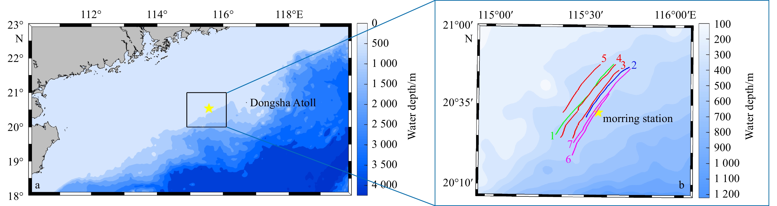
From July 10 to 13, 2017, satellite sensors with spatial resolution ranging from 5 m to 250 m captured several ISW packets on the slope of the NSCS with water depth of 300−400 m. These sensors include the panchromatic camera (PAN) onboard China-Brazil Earth Resource Satellite-4 (CBERS-4), wide field of view (WFV3) sensor onboard Chinese GaoFen-1 (GF-1), Enhanced Thematic Mapper Plus (ETM+) onboard Landsat-7 and MODIS onboard Terra/Aqua satellites. As shown in Fig. 1, total seven images were collected. Their observation time and spatial resolution are listed in Table 1. One can see that the ISWs are clearly shown as alternating bright and dark curves and propagated westwards. On 12 July, the same ISW packet was continuously observed by CBERS-4, GF-1 and MODIS (Figs 1c-e) within two and a half hours. One day later, Landsat-7 ETM+ and MODIS detected another ISW packet at almost the same time.

Figure  1.  Satellite images of the internal solitary waves in the northern South China Sea. MODIS images were acquired on July 10 (a), July 11 (b), July 12 (e) and July 13, 2017 (g); CBERS-4 image (c) and GF-1 image (d) were acquired on July 12, 2017; Landsat-7 image (f) was acquired on July 13, 2017.

DownLoad: Full-Size Img PowerPoint

Table  1.  Information of satellite images

Image No.	Image ID	Time	Satellite (senor)	Spatial resolution/m
1	M0710	July 10, 2017, 05:30 UTC	Aqua (MODIS)	250
2	M0711	July 11, 2017, 03:10 UTC	Terra (MODIS)	250
3	C0712	July 12, 2017, 02:59 UTC	CBERS-4 (PAN)	5
4	G0712	July 12, 2017, 03:37 UTC	GF-1 (WFV3)	16
5	M0712	July 12, 2017, 05:20 UTC	Aqua (MODIS)	250
6	L0713	July 13, 2017, 02:43 UTC	Landsat-7 (ETM+)	15
7	M0713	July 13, 2017, 02:55 UTC	Terra (MODIS)	250

 | Show Table

DownLoad: CSV

2.1.2   Mooring observations

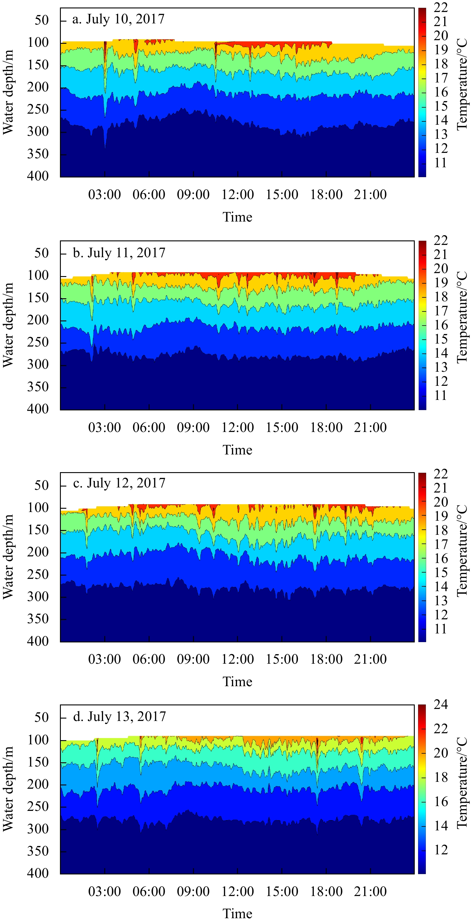
The ISWs observed by different satellites were also recorded by a mooring deployed at 20.542°N, 115.574°E in the west of the Dongsha Atoll as shown in Fig. 2. The vertical profiles of water temperature below 90 m concurrently measured by the mooring chain of conductivity-temperature-depth (CTD) instruments from July 10 to 13, 2017 are shown in Fig. 3. One can see that the warmer waters in the upper layer were depressed into the lower layer, showing the existence of solitary depression wave packets clearly. For example, at about 1:30 UTC in Fig. 3c, a pulse of 18°C isotherm depressed quickly from 110 m to 156 m within 15 min.

Figure  2.  Location of the mooring station (yellow pentagram) and crest lines (color lines) of the leading ISWs extracted from satellite images in the northern South China Sea. Numbers 1 to 7 denote the ISWs on Images 1 to 7 in Table 1, respectively.

DownLoad: Full-Size Img PowerPoint

Figure  3.  Vertical profiles of water temperature measured by the mooring CTD chain deployed near Dongsha Atoll in the northern South China Sea from July 10−13, 2017.

DownLoad: Full-Size Img PowerPoint

2.1.3   Ocean reanalysis data and bathymetry data

To extract the ISW amplitude from satellite images, the ocean stratification data are necessary. In this study, the global reanalysis data provided by the Copernicus Marine Environment Monitoring Service (CMEMS) (http://marine.copernicus.eu) are used for calculating the upper layer depth. This product is the global ocean eddy-resolving reanalysis with (1/12)° horizontal resolution and 50 vertical levels based on joint assimilation of along-track altimeter data, satellite sea surface temperature, sea ice concentration and in situ temperature and salinity profiles. It contains three-dimensional daily mean fields of temperature, salinity and current, and covers the period when altimetry data are available (Lellouche et al., 2018).

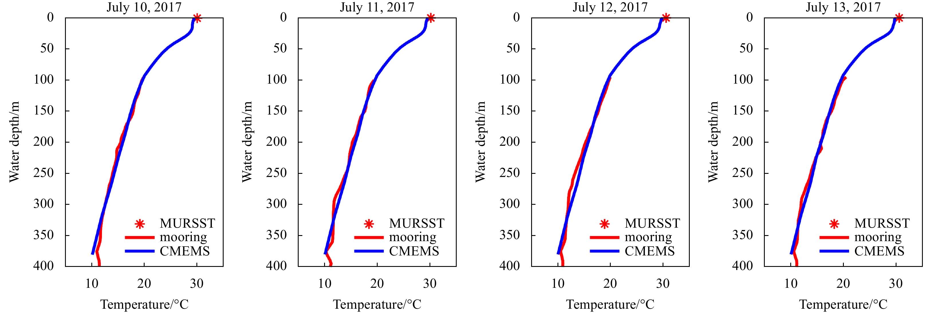
Daily multi-scale ultra-high resolution sea surface temperature data with spatial resolution of about 0.01° (Chin et al., 2017) developed by Jet Propulsion Laboratory/National Aeronautics and Space Administration, as well as the mooring measurements, are used to evaluate the accuracy of CMEMS data in the study area. As shown in Fig. 4, one can see that the reanalysis datasets reproduce the sea surface temperature and mooring observed vertical profiles of temperature well.

Figure  4.  Comparisons of daily multi-scale ultra-high resolution sea surface temperature (MURSST), mooring observed temperature and Copernicus Marine Environment Monitoring Service (CMEMS) temperature at the mooring location during July 10−13, 2017.

DownLoad: Full-Size Img PowerPoint

For the two-layer ocean approximation, once the upper layer depth h₁ is calculated from the CMEMS data, the lower layer depth h₂ can be obtained by subtracting this value from the total water depth h, which comes from the ETOPO1 data (https://www.ngdc.noaa.gov/mgg/global/global.html) with spatial resolution of 1 arc-minute (Amante and Eakins, 2009).

2.2 Estimation of ISW amplitudes from satellite images

In this study, the KdV and the NLS equations are used to extract the ISW amplitude from satellite images to assess their suitability under a given circumstance using in situ measurements as a standard.

2.2.1   KdV equation approach

In a two-layer fluid, the KdV equation (Ostrovsky and Stepanyants, 1989) can be expressed as

where $\eta (x,t)$ is the vertical displacement of the ISW as a function of horizontal displacement x and time t; and the linear phase speed

${\alpha _1}$ is defined as the nonlinear parameter, which can be expressed as

${\beta _1}$ is defined as the dispersive parameter, which can be expressed as

Here g is the gravitational acceleration; ${\rho _1}$ and ${\rho _2}$ are the water densities of the upper and lower layers, respectively.

The solution of Eq. (1) is

where ${\eta _0}$ is the initial amplitude of the ISW; V is the nonlinear phase speed:

Δ is the characteristic half width:

The characteristic half width has a relation with the distance l between the brightest spot and the darkest spot (hereafter called peak-to-peak distance) of the ISW crest lines on a satellite image (Zheng et al., 2001) which can be expressed as

Combining Eq. (7) and Eq. (8), the amplitude of the ISWs can be obtained by

2.2.2   NLS equation approach

The NLS equation derived from the dynamic equation of two-layer fluid (Pelinovsky, 1995; Zhang et al., 2016) is expressed as

where the nonlinear parameter

and the dispersive parameter

Here ${\alpha ^{(2)}}$ and ${\ \beta ^{(2)}}$ are the correction terms introduced to the nonlinear parameter and dispersive parameter; $\varepsilon $ is a small parameter; $\omega $ is the frequency

and

where k is the wave number; c₁, f₃, f₆, f₇ and f₂₅ are coefficients produced during the deviation, and the group velocity of the ISW is

There are two possibilities for the solution of Eq. (10). When ${\alpha _2}{\beta _2} > 0$, the solution is

where the characteristic half width

When ${\alpha _2}{\beta _2} < 0$, the solution is

where the characteristic half width

The peak-to-peak distance is 1.76 times of the characteristic half width here for ${\alpha _2}{\beta _2} > 0$, i.e., $l = 1.76\varDelta $. For ${\alpha _2}{\beta _2} < 0$, $l = 1.{\text{32}}\varDelta $. Therefore, the amplitude of the ISW on a satellite image is obtained by

3. Results and discussion

3.1 Amplitudes of ISWs

With Eq. (9) or Eq. (20), the amplitude of an ISW can be estimated based on the peak-to-peak distance extracted from a satellite image and values of nonlinear and dispersive parameters calculated from CMEMS and ETOPO data. For each ISW, the center position of the leading crest line on the image is taken as its location. Table 2 lists the water depth where satellite-observed ISWs occurred, the peak-to-peak distance extracted from these images, and the derived ISW amplitudes by using the KdV and NLS equation approaches. Compared with mooring measurements, the characteristics of ISW packets on three high-resolution images are well described by the KdV equation, meanwhile the amplitudes of ISWs estimated from MODIS images using the NLS equation approach are all in better agreement with the mooring observations. The amplitudes of the same ISW packets calculated by the two methods, however, are quite different. The maximum deviation reaches up to one order of magnitude. Hereafter, the reasons to cause the difference and the suitability of the two methods will be analyzed.

Table  2.  The characteristic parameters of the ISWs observed by satellites and the mooring CTD chain

Image ID	Water depth/m	l/m	Amplitude/m
			S-KdV	S-NLS	Mooring
M0710	370	500	4.9	55.1	68.5
M0711	390	750	2.3	44.0	48.1
C0712	390	175	42.0	189.6	45.7
G0712	370	176	39.4	158.4	45.7
M0712	327	500	4.3	34.3	45.7
L0713	408	120	67.9	419.5	66.1
M0713	398	750	1.7	61.9	66.1
Note: l is the peak-to-peak distance; S-KdV and S-NLS are amplitudes estimated using the KdV and the NLS equation approaches, respectively; the number in bold represents that the estimated amplitude is closer to the mooring observation.

 | Show Table

DownLoad: CSV

From the seven cases listed in Table 2, one can see that the accuracies of the two methods in estimating the ISW amplitude seem to be slightly associated with the spatial resolution of satellite images. According to the theoretical expressions Eqs. (9) and (20), the amplitude obtained by the KdV equation is inversely proportional to the square of the peak-to-peak distance, rather than to the peak-to-peak distance itself as described in the NLS equation. As a result, the accuracy of the KdV equation derived amplitude is more dependent on the measurement of the peak-to-peak distance or the characteristic half width, which can be extracted more accurately from images with higher spatial resolution.

Table 3 lists details of results by previous investigators. Huang and Zhao (2014) analyzed the characteristics of an ISW packet in deep waters of the SCS based on a MODIS image with 250 m resolution. They used the KdV equation approach to calculate the ISW amplitude and obtained the results very close to the field observation with a relative error of only 1.6%. Li et al. (2013) estimated the amplitude of an internal wave in Malin Shelf from an ERS-1 SAR image with spatial resolution of 30 m using the NLS equation approach and the obtained result agreed fairly well with the in situ measurement. All these studies indicate that there are other reasons leading to the large difference in the amplitudes derived by the KdV and the NLS equation approaches. Thus, it is necessary to determine the criterion and certain conditions for application of these two methods.

Table  3.  ISW amplitudes derived from satellite observations in previous studies

Literature	Satellite (sensor)	Spatial resolution/m	Region	Water depth/m	l/m	Amplitude/m
						KdV	NLS	Observation
Small et al. (1999)	ERS-1 (SAR)	30	Malin Shelf	500	350	24.2	−	49.0
				600	400	26.0	−	49.0
				700	400	31.7	−	49.0
				500	350	49.6	−	30.0
Zheng et al. (2001)	ERS-1 (SAR)	30	Portugues Continental Shelf	140	110	26.0	−	23.0
				140	220	7.0	−	10.0
				140	240	6.0	−	5.0
	Radarsat-1 (SAR)	100	SCS	350	900	48.0	−	−
				350	1100	37.0	−	−
Li et al. (2008)	Envisat (ASAR)	150	SCS	70	99	8.0	−	6.0−10.0
Li et al. (2013)	ERS-1 (SAR)	30	Malin Shelf	500	350	−	42.2	49.0
				600	400	−	37.8	49.0
				700	400	−	40.8	49.0
Huang and Zhao (2014)	Aqua (MODIS)	250	SCS	3179	4301	124.0	−	126.0
Zhang et al. (2016)	Envisat (ASAR)	150	SCS	92	317	0.7	18.1	18.0
	Aqua (MODIS)	250		117	882	−	14.2	15.0
Note: l is the peak-to-peak distance; − represents no data.

 | Show Table

DownLoad: CSV

Here we define a determination parameter $\chi $ as

where $ A = \dfrac{{4\pi h_1^2h_2^2}}{{3{\varDelta ^2}h\left( {{h_2} - {h_1}} \right)}} $ is the dimensionless nonlinear parameter and $B = {\left( {\dfrac{h}{{\pi \varDelta }}} \right)^{ 2}}$ is the dimensionless dispersive parameter (Lee and Beardsley, 1974). Substituting A and B into Eq. (21) yields

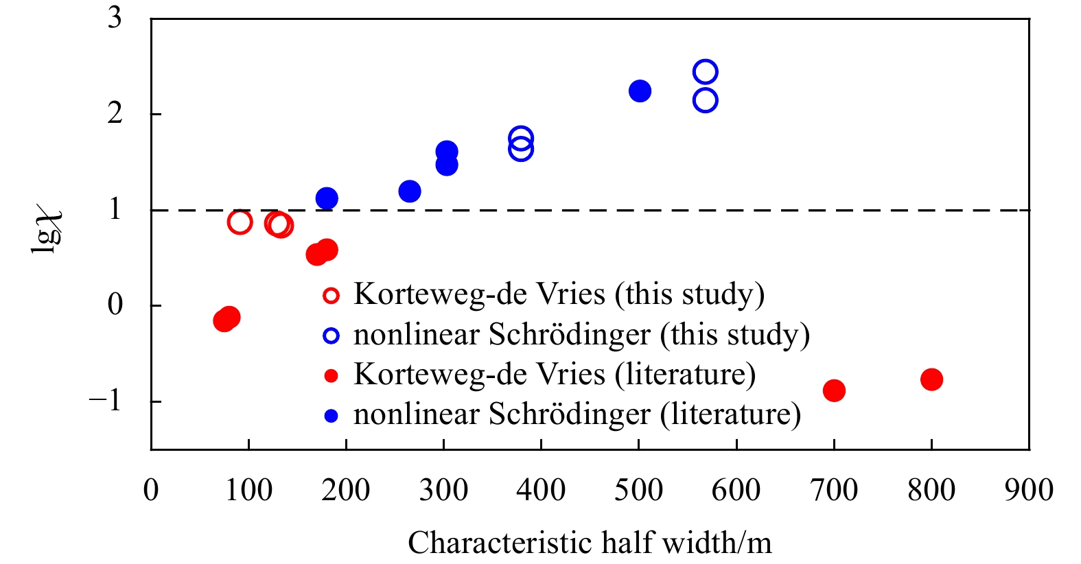
Figure 5 shows a scatter plot of lg$\chi $ and characteristic half width of ISWs. The data points include the results derived from this study and that from the literature (Zheng et al., 2001; Li et al., 2008, 2013; Zhang et al., 2016). One can see that the data points are divided into two groups bounded by a line of lg$\chi $=1. The upper group for lg$\chi $>1 is corresponding to the cases, in which the NLS equation approach gives more accurate estimates of ISW amplitudes. The lower group for lg$\chi $<1 corresponds to the cases, in which the KdV equation approach gives more accurate estimates. This result implies that the determination parameter $\chi $ may serve as a good criterion to assess the suitability of the two amplitude estimation methods.

Figure  5.  A scatter plot of lg$\chi $ and characteristic half width of ISWs. Open and solid circles represent the data derived from this study and cited from previous studies, respectively.

DownLoad: Full-Size Img PowerPoint

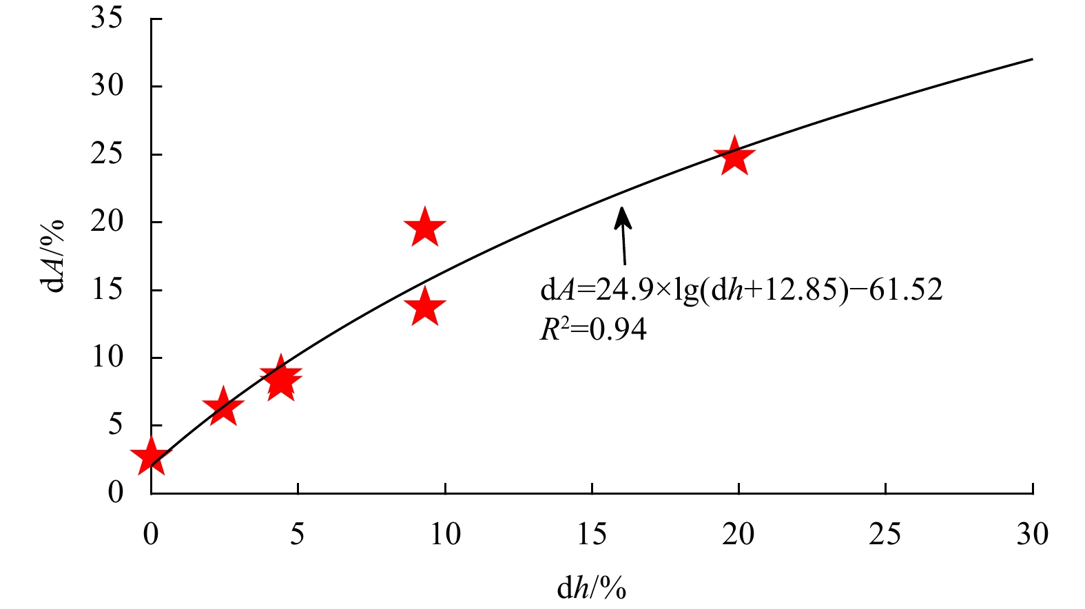
Furthermore, the errors of the ISW amplitudes estimated from seven satellite images using the KdV and the NLS equation approaches are analyzed based on the above criterion. The results are shown in Table 4 and Fig. 6. One can see that the relative error (dA) of satellite observed amplitudes with respect to the mooring observations ranges from 2.7% to 24.8% and is highly associated with the bottom slope, which is defined as $ \text{d}{h}{=}\text{|}{{h}}_{\rm{s}}{-}{{h}}_{\rm{o}}\text{|}/{{h}}_{\rm{o}} $, where $ {{h}}_{\rm{s}} $ and $ {{h}}_{\rm{o}} $ are the depths at satellite observed ISW location and the mooring station. The determination coefficient R² of the logarithmic fit curve in Fig. 6 is 0.94, indicating a close relation of the ISW amplitude error to the bottom slope. This may be attributed to the ISW dissipation during their evolution process along a shoaling topography or thermocline (Zheng et al., 2007; Geng et al., 2019; Xie et al., 2019).

Table  4.  The relative error of satellite estimated ISW amplitude and bottom slope

Image ID	Relative error dA/%	Bottom slope dh/%
M0710	19.5	9.3
M0711	8.7	4.4
C0712	8.1	4.4
G0712	13.7	9.3
M0712	24.8	19.9
L0713	2.7	0
M0713	6.3	2.5

 | Show Table

DownLoad: CSV

Figure  6.  Relation of the relative error (dA) of satellite estimated ISW amplitude to the bottom slope (dh). Data points represent the results of ISWs observed on the seven satellite images during July 10−13, 2017.

DownLoad: Full-Size Img PowerPoint

3.2 Propagation of ISWs

The propagation speed is an important parameter of the ISWs, which can be calculated by the KdV Eq. (6) and the propagation distance measured from two consecutive satellite images with a known time interval (Liu et al., 2014). In cases that in situ measurements are available, this information together with the satellite observation can be also used to obtain the propagation speed (Huang and Zhao, 2014). In this study, the detection of the same ISW packet by multiple satellite images with concurrent mooring observations provides a great opportunity to investigate the propagation characteristics of ISWs. In addition to the above methods, a distance-weighted averaging method is also used to calculate the propagation speed of the ISWs observed by CBERS-4/PAN, GF-1/WFV3 and MODIS on July 12, 2017 (Figs 1c-e). With this method, the propagation speed V of an ISW packet observed by the second satellite image is expressed as

where ${V_1} = {{{d_1}}/ {\Delta {t_1}}}$ and ${V_2} = {{{d_2}}/ {\Delta {t_2}}}$ are the propagation speeds calculated from the first or last two consecutive images acquired at a time interval of Δt₁ or Δt₂ with a distance of d₁ or d₂, respectively; $ {w_1} = \dfrac{{{d_2}}}{{{d_1} + {d_2}}} $ and $ {w_2} = \dfrac{{{d_1}}}{{{d_1} + {d_2}}} $ are the corresponding weighted coefficients.

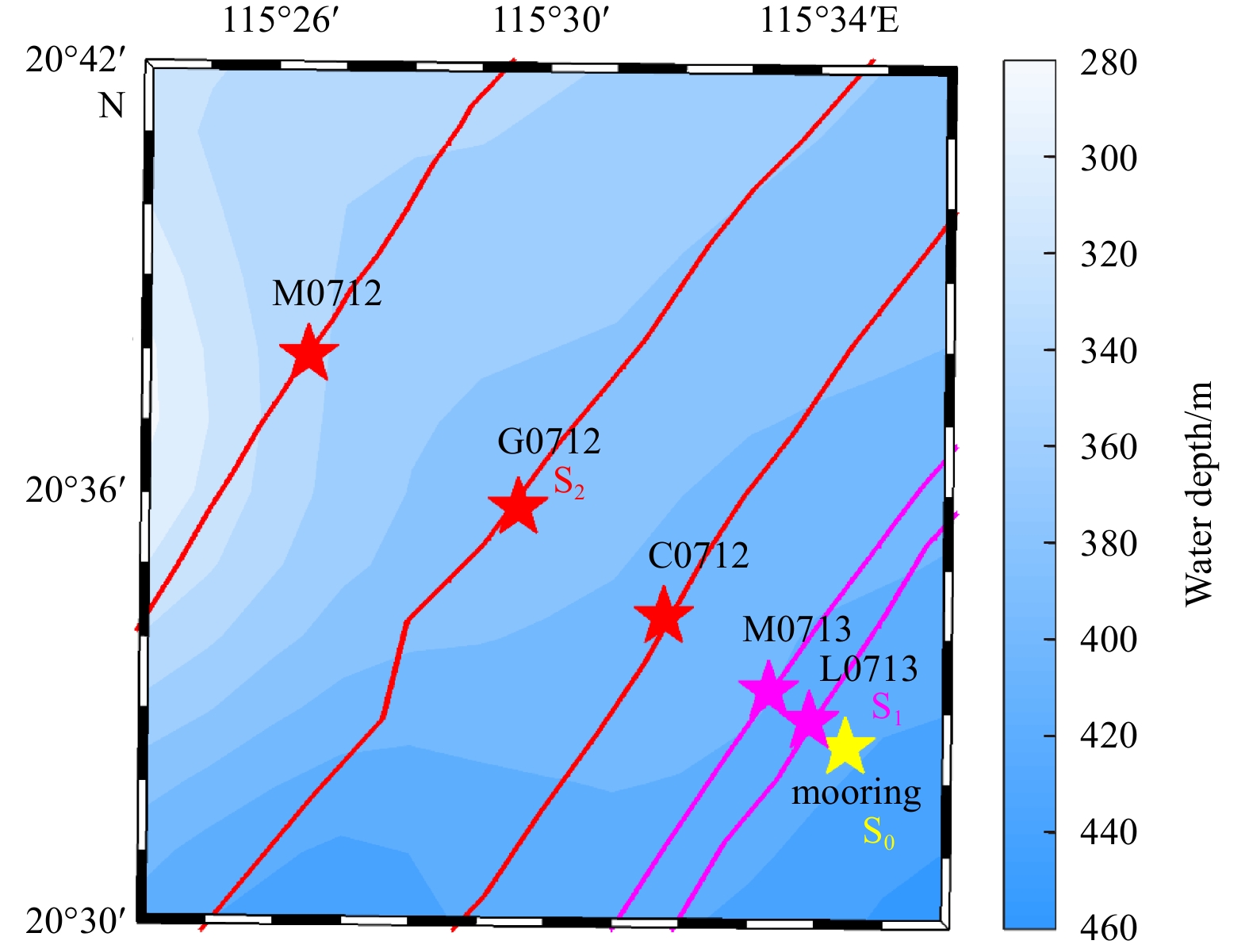
Figure 7 shows the mooring location and leading ISW crest lines observed by the satellites. The time interval between three satellite images is shorter than 3 h. As mentioned in the previous section, the characteristics of ISWs on CBERS-4 and GF-1 images can be well described by the KdV equation, thus the propagation speeds of ISWs observed by CBERS-4 and GF-1 should be consistent with the theoretical results by Eq. (6). Table 5 lists the propagation speeds of the ISWs at CBERS-4 and GF-1 locations. One can see that the results derived from different methods are comparable to the theoretical propagation speeds derived from the KdV equation. Particularly, the phase speeds retrieved from multiple satellite images or satellite and in situ observations are much closer to the theoretical results, demonstrating the advantage of multiple observations (i.e., >2 observations) in ISW phase speed estimation. At CBERS-4 and GF-1 locations, the relative errors of the mean propagation speeds are 4.9% and 0.6% with respect to the theoretical results, respectively.

Figure  7.  Locations of the mooring station (yellow pentagram), ISWs observed by CBERS-4/PAN (C0712), GF-1/WFV3 (G0712) and Aqua/MODIS (M0712) (red pentagrams) on July 12, 2017 and Landsat-7/ETM+ (L0713) and Terra/MODIS (M0713) (purple pentagrams) on July 13, 2017. The locations of the mooring station and ISWs observed by Landsat-7/ETM+ on July 13 and GF-1/WFV3 on July 12 are marked as S₀, S₁ and S₂.

DownLoad: Full-Size Img PowerPoint

Table  5.  Propagation speeds of the ISWs at CBERS-4 and GF-1 locations

	Data sources	Satellite derived propagation speed/(m·s−1)	KdV-derived propagation speed/(m·s−1)
CBERS-4	CBERS-4 and GF-1	2.04	1.62
	CBERS-4 and MODIS	1.34
	CBERS-4, GF-1 and mooring	1.73
	mean	1.70±0.35
GF-1	GF-1 and CBERS-4	2.04	1.58
	GF-1 and MODIS	1.08
	GF-1, CBERS-4 and MODIS	1.65
	mean	1.59±0.48

 | Show Table

DownLoad: CSV

3.3 Type of ISWs

As shown in Fig. 2, the ISWs on the seven satellite images from July 10 to 13, 2017 occurred in almost the same geographical region. Therefore, there might not be much difference in their propagation speed especially on the same day. The locations of the mooring station and ISWs observed by Landsat-7/ETM+ on July 13 and GF-1/WFV3 on July 12 are marked as S₀, S₁ and S₂ in Fig. 7, respectively. When the ISW packet passed S₀, it was recorded by the mooring chain. With the propagation speed derived from the KdV equation, the wave arrival time at S₁ or S₂ can be estimated and used to determine the type of the ISWs as listed in Table 6. The most significant difference between three types of ISWs is the re-appearance period, which is about 24 h for type-A ISWs, 25 h for type-B ISWs and 23 h for type-C ISWs. In addition, some statistics show that the amplitude of type-B ISWs is larger than that of type-A and type-C ISWs (Chen et al., 2018). In Table 6, each row represents the ISW arrival time on the same day at different locations and each column represents the ISW arrival time at the same location on different days. One can see that the ISWs arrived at S₀, S₁ and S₂ earlier each day from July 10 to 12, implying that the waves were all type-C ISWs. This is consistent with the mooring observations. On the other hand, the ISW arrival time at S₀, S₁ and S₂ was delayed by about 43 min, 26 min and 42 min on July 13 compared with that on July 12, implying that the wave was a type-B ISW.

Table  6.  The time that the ISWs passed the locations of the mooring (S₀), Landsat-7 (S₁) and GF-1 (S₂)

	Time at S0	Time at S1	Time at S2
July 10, 2017	03:01	04:10	05:27
July 11, 2017	02:08	02:42	04:13
July 12, 2017	01:48	02:17	03:37
July 13, 2017	02:31	02:43	04:19
Note: Time at S0 is mooring measured. The number in italic represents the ISW arrival time at S1 or S2 calculated by the phase speed derived from the KdV equation. The number in bold represents satellite-imaging time.

 | Show Table

DownLoad: CSV

4. Conclusions

This study aims to assess the accuracy and the applicability of theoretical approaches including the KdV and NLS equation solutions to derivation of dynamic parameters of internal solitary waves from satellite images. Multi-satellite images and concurrent mooring observations near the Dongsha Atoll of the NSCS from July 10 to 13, 2017 are used as a baseline, from which the amplitudes of ISWs are estimated by the KdV and the NLS equation solutions. The assessment results and major findings are summarized as follows.

(1) We propose the ratio of the dimensionless dispersive parameter to the square of dimensionless nonlinear parameter $\chi $ to serve as a criterion, which is used to assess the accuracy and the applicability of the KdV and NLS equation approaches to estimating the ISW amplitudes based on the characteristic half width extracted from the satellite images. The statistics of total 18 cases indicate that in 50% of cases for lg$\chi $>1, the NLS approach gives more accurate estimates of ISW amplitudes and in the other 50% of cases for lg$\chi $<1, the KdV approach does.

(2) We find that the relative errors of ISW amplitudes derived from the KdV or NLS approach are closely associated with the logarithmic bottom slopes. This may be attributed to the nonlinear growth of ISW amplitudes as the waves propagate along a shoaling thermocline or topography (Zheng et al., 2007). Thus, proper determination of the slopes of shoaling thermocline or topography is a key factor for improving the accuracy of ISW amplitude estimation.

(3) The test results using three consecutive satellite images to retrieve the ISW propagation speeds indicate that the use of multiple satellite images (>2) may improve the accuracy of retrieved phase speeds. Meanwhile, repeated multi-satellite images of ISWs can help to determine the types of ISWs if mooring data are available nearby.

With the improvement of the temporal and spatial resolution of satellite images, remote sensing is now playing an increasingly important role in the study of ISWs. In the near future, more data including SAR images with spatial resolution up to 1 m, such as Chinese Gaofen-3 SAR, will be collected for further investigation of the wave parameter estimation methods and wave characteristics.