High-resolution simulation of upper-ocean submesoscale variability in the South China Sea: Spatial and seasonal dynamical regimes

1. Introduction

Upper-ocean submesoscale processes, with horizontal scales of a few to tens of kilometers and time scales of a few days, are ubiquitous in the ocean and have strong impacts on the oceanic flows. A number of studies have revealed that submesoscale processes play a key role in the restratification of mixed layer (ML) (Boccaletti et al., 2007; Fox-Kemper et al., 2008; Bachman et al., 2017), oceanic vertical transport of salt, heat, biogeochemical productivity (Mahadevan and Tandon, 2006; Lévy et al., 2012; Zhong and Bracco, 2013; Rosso et al., 2014; Siegelman et al., 2020), and energy transfer to smaller scales (Capet et al., 2008; Cao et al., 2021). Understanding these effects is crucial to the upper-ocean mixing (Yang et al., 2017), planktonic ecosystem (Lévy et al., 2018), and oceanic energy cycle (Dong et al., 2020; Cao et al., 2021). Some other studies through numerical simulations (Sasaki et al., 2014; Brannigan et al., 2015; Rocha et al., 2016; Wang et al., 2018; Zhang et al., 2020) and observations (Callies et al., 2015; Thompson et al., 2016; Yu et al., 2019) have shown that the upper-ocean submesoscale processes undergo a clear seasonal cycle depending on the local background flow and forcing. Submesoscale physics are ubiquitous but highly heterogeneous in space and time.

Strong, dense submesoscale processes can be generated in regions where the lateral buoyancy gradient or strain rate is strong. The former can provide sufficient potential energy (fronts) that catalyzes instabilities with energy transfer to smaller scales, and the latter is favorable for generating submesoscale fronts (known as submesoscale frontogenesis). The two processes frequently occur in or near western boundary currents (D’Asaro et al., 2011; Shcherbina et al., 2013), in the Southern Ocean (Adams et al., 2017), and in marginal seas (e.g., the South China Sea, hereafter referred to as SCS; Zhang et al., 2020). Physically, these effects arise from a series of submesoscale instabilities that extract energy from the background flow (Haine and Marshall, 1998).

In the open ocean, the seasonality of submesoscale activities highly depended on the modulation of the climatological forcing (Sasaki et al., 2014), while in marginal seas, submesoscale behaviors can be generated and modulated by some other regimes like river runoff, intrusion flows, and bottom topography. For example, Barkan et al. (2017) investigated the submesoscale flows driven by the Mississippi–Atchafalaya River system on and off the Gulf of Mexico. Zhang et al. (2020), using a submesoscale-permitting simulation, reported the submesoscale characteristics in the northern SCS. In this study, we ran a high-resolution model to provide more details of the submesoscale processes over the whole SCS, aiming at investigating the regional and seasonal differences of submesoscale variability over the whole SCS.

The SCS, known as the largest semi-enclosed marginal sea in the tropical western Pacific Ocean, has broadly distributed mesoscale eddies (Wang et al., 2003; Chen et al., 2011; Nan et al., 2011a, 2011b; Xie and Zheng, 2017). The energetic dynamical activities are attributed to several complex mechanisms: (1) External fluxes from the western Pacific Ocean via the Luzon Strait (Qu and Lukas, 2003; Tian et al., 2006; Hu et al., 2012), (2) seasonally reversing monsoon forcing (Hu et al., 2000, 2020), (3) complex bottom topography. Previous studies tended to emphasize the mesoscale processes in the SCS, and in effect, there also exist energetic submesoscale eddies, fronts/filaments, and topographic wakes. Zheng et al. (2020) reviewed the research progress in oceanic submesoscale physics in this region. However, most of these studies paid their attention to the northern SCS (Cao et al., 2019; Li et al., 2019; Zhang et al., 2020, 2021b), and only a few of them studied the western SCS (Yu et al., 2018; Huang et al., 2020). To our knowledge, few studies are reported with particular attention to the southern SCS. Our understanding of the mechanisms controlling the seasonal variations of submesoscale processes in the SCS is still limited.

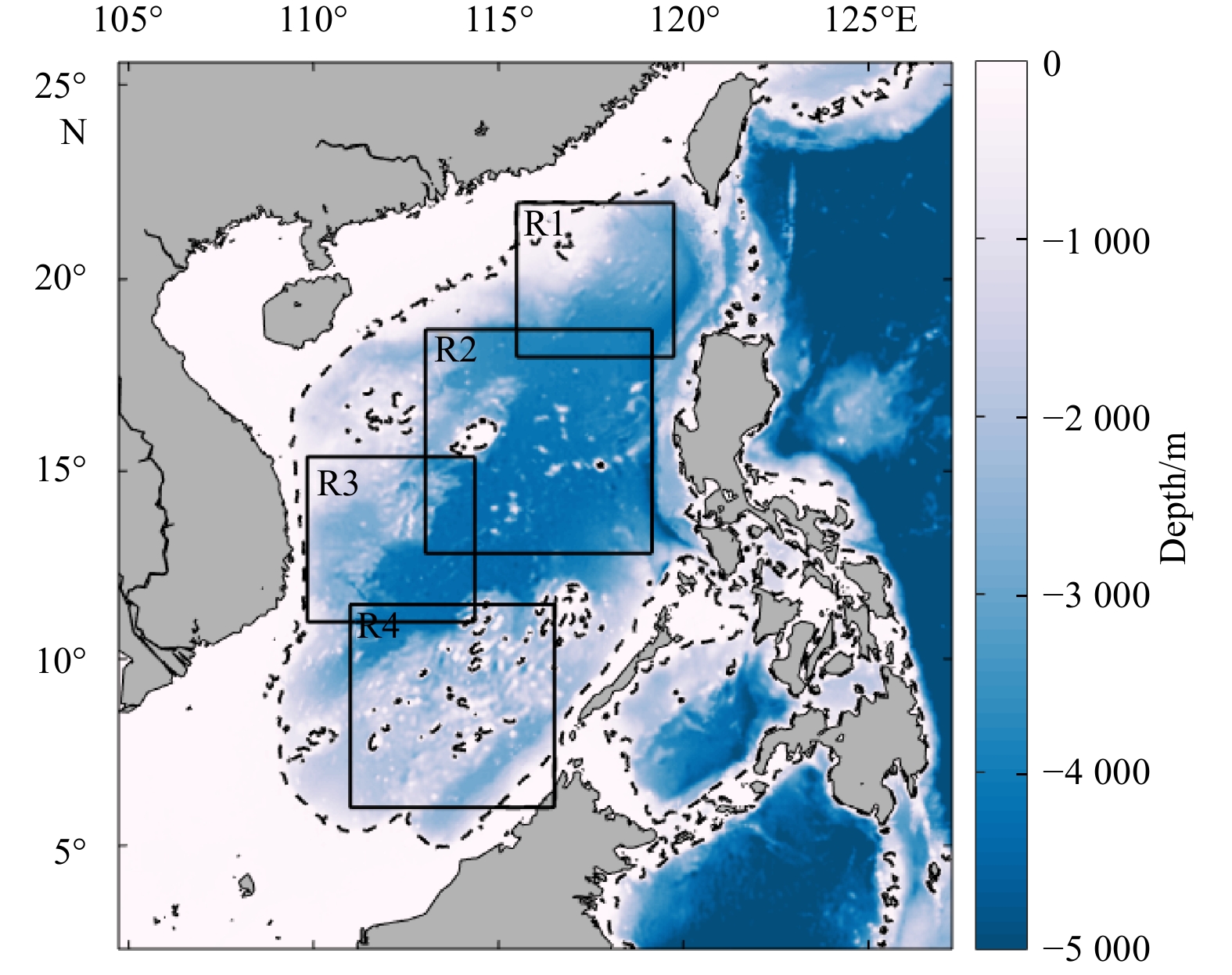
In this paper, the SCS is classified into four sub-regions: the region west of the Luzon Strait (R1), the middle ocean basin (R2), the western SCS (R3), and the southern SCS (R4) as shown in Fig. 1. As also discussed in Yang et al. (2021), the upper-ocean submesoscale physics (e.g., submesoscale eddies and fronts) for each sub-region is investigated via a high-resolution simulation (horizontal grid size of ~1.5 km). This paper further investigates the spatial and seasonal differences of submesoscale characteristics and explores the dynamical relations between the submesoscale features and the local background flow and forcing for each sub-region to improve the understanding of different regimes for submesoscale physics in the sub-regions. The rest of the paper is organized as follows. Section 2 describes the numerical configurations. Section 3 presents the seasonal differences of the submesoscale characteristics such as enhanced vertical vorticity, horizontal divergence, straining rate, lateral buoyancy gradient, and vertical velocity. The Ertel potential vorticity (PV) of several typical sections is also studied to elucidate the generation mechanisms of submesoscale processes in different sub-regions. In Section 4, the correlations between the variables within (z = −10 m) and below (z = −150 m) the ML are investigated, and the vertical extent of vertical velocity and the SCS monsoon index are also examined in the correlation analysis. Summary appears in Section 5.

Figure  1.  Bathymetry of South China Sea (SCS). The boxes with solid lines marked the four sub-regions known as the northern SCS (R1), the ocean basin (R2), the western SCS (R3), and the southern SCS (R4).

DownLoad: Full-Size Img PowerPoint

2. Model setup

The Regional Oceanic Modeling System (ROMS) is used to conduct a nesting simulation from a parent model (ROMS0). The parent model covers the entire western Pacific and was run on a curvilinear, latitude–longitude grid and terrain-following S-coordinates of 60 vertical levels, with a horizontal resolution of ~7.5 km. The ROMS0 has run for 20 years (spin-up) to reach a statistically equilibrated state before starting the nesting simulations on a child grid of ~1.5 km (ROMS1). The sub-grid vertical mixing of tracers and momentum is based on the K-profile parameterization scheme (Large et al., 1994). All of these nested models have a daily mean output in the 21st model year. The surface atmospheric forcing (e.g., wind stress, heat, and freshwater fluxes) were provided by the daily mean climatology of the Quick Scatterometer (QuikSCAT) dataset and the International Comprehensive Ocean Atmosphere Dataset (ICOADS) (Woodruff et al., 2011). The boundary and initial information for ROMS0 were from the monthly averaged Simple Ocean Data Assimilation (SODA) ocean climatology outputs (Carton and Giese, 2008). The bathymetry data for all the domains are obtained from the British Oceanographic Data Centre (https://www.bodc.ac.uk/data/) based on the 30 arc-s dataset of General Bathymetric Chart of the Oceans. The modeling results, including regional circulation, thermohaline structure, mixed layer depth (MLD), and energy level of mesoscale eddies, have been validated against the available satellite and reanalysis datasets before the analysis of this study, as well as the limited in situ observations in the SCS and the northwestern Pacific Ocean. The comparisons to measurements on multiple platforms show that the simulations are sufficiently accurate to characterize the seasonal conditions. Also, the nested simulations have been used for analysis by several studies (e.g., the Kuroshio Extension, Luo et al., 2020; Cao et al., 2021; the western SCS, Yu et al., 2018; Huang et al., 2020; the Subtropical Countercurrents, Jing et al., 2021). In this study, the one-year simulation over the whole SCS is used to analyze the submesoscale features in the SCS. In Huang et al. (2020), the simulated mesoscale eddy kinetic energy level in the SCS was validated with the satellite altimeter data and the submesoscale fronts were also compared to the Medium Resolution Imaging Spectrometer images and the high-resolution sea surface temperature data distributed by the Group for High Resolution Sea Surface Temperature project.

3. Submesoscale characteristics

3.1 Vertical vorticity, horizontal divergence, strain rate, and density fronts

Figure 2 shows the snapshots of vertical vorticity normalized by f for three depth levels on January 15 and July 15, respectively. The −10 m layer represents the ML, the depth of −50 m is roughly around the base of the ML, and the −200 m layer is well below the ML. The results show that the vertical vorticity is highly heterogeneous in the SCS, with higher values near the coast. The northern SCS (R1) exhibits more submesoscale eddies in winter than in summer. This region is favorable for generating mesoscale eddies due to the influence of intrusion flows through the Luzon Strait (Hu et al., 2000; Qu et al., 2000; Xue et al., 2004; Wang et al., 2006; Nan et al., 2011b), with submesoscale eddies in the periphery of mesoscale eddies (the zoom-in plot in Fig. 2b). The submesoscale flows would largely associated with the mesoscale eddies. In contrast, the upper-ocean submesoscale processes in the SCS basin (R2) are less influenced by the Pacific flows but modulated by the local seasonally-varying atmosphere forcing (this will be demonstrated in Section 4). In the west (R3), an elongated cold filament is frequently formed off the coast (the zoom-in plot Fig. 2d), primarily attributed to the sheared flow associated with the summer southwestern monsoon (Xie et al., 2003; Li et al., 2017). This will result in secondary barotropic and baroclinic instabilities at the submesoscales, e.g., the vortex trains studied by Yu et al. (2018). Notice that the filamentous structures remain clear at z=−200 m (Fig. 2f), although most of the submesoscale features are largely declined. In the southern SCS (R4) where multi-islands are located, topography wakes could be easily generated via the current-topography interaction. Hence, even at depths, the submesoscale behaviors in R4 are still active near the islands, although they are weakened on average.

Figure  2.  Snapshots of vertical vorticiy ζ/f at z=−10 m, −50 m, and −200 m on January 15 (winter) and July 15 (summer). The boxes with solid black lines in the first plot mark out the sub-regions: R1, R2, R3, and R4. Here z is the water depth.

DownLoad: Full-Size Img PowerPoint

The horizontal divergence of the flow ($\text{δ} {\text{ = }}{u_x} + {v_y}$) shows smaller scales than the vertical vorticity and is strongest at the near-surface layer, indicating the growing unbalanced motions (Fig. 3). A comparison between the summer and winter divergence fields shows that the northern SCS displays clear seasonal differences, which are not as apparent in the southern region (Figs 3a, d). This is consistent with the seasonality of the vertical vorticity field (Fig. 3 compared to Fig. 2). There appears strong flow strain in the SCS due to the regional circulation and outer forcing. In detail, the strain rate, $ S = \sqrt {{{({u_x} - {v_y})}^2} + {{({u_y} + {v_x})}^2}} $, exhibits rich filamentous structures at submesoscales (Fig. 4), favorable for generating submesoscale fronts. Here the original velocity is used in calculating the strain rate. In particular, the mesoscale eddies stimulate strong straining at the eddy rings that extends to the deep (e.g., in R1). Notice that the southern islands in R4 remarkably strengthen the straining field, with denser, smaller structures. During the summertime, the aforementioned filament in R3 can also be observed with vortical shapes of enhanced strain rates nearby (Fig. 4d).

Figure  3.  Snapshots of horizontal divergence $\text{δ} $/f at z=−10 m, −50 m, and −200 m on January 15 (winter) and July 15 (summer). The boxes with solid black lines in the first plot mark out the sub-regions: R1, R2, R3, and R4. Here z is the water depth.

DownLoad: Full-Size Img PowerPoint

Figure  4.  Snapshots of strain rate S/f at z=−10 m, −50 m, and −200 m on January 15 (winter) and July 15 (summer). The boxes with solid black lines in the first plot mark out the sub-regions: R1, R2, R3, and R4. Here z is the water depth.

DownLoad: Full-Size Img PowerPoint

There appears denser, stronger mixed-layer (z=−10 m) buoyancy gradient, $ \left| {\nabla b} \right| $, to the north than to the south, distinct from the spatial pattern of the vorticity field (Fig. 5). This suggests that the northern SCS has more energetic submesoscale fronts especially in the winter mixed layer (Dong and Zhong, 2020), likely due to the stronger intrusion flow that generates stronger buoyancy gradients for this region during wintertime. This would also provide substantial available potential energy for generating submesoscale eddies. However, the strong mixed-layer submesoscale eddies in the south partly result from barotropic processes, e.g., topography wakes. The buoyancy gradient at the base of mixed layer (z=−50 m) is remarkably enhanced (Fig. 5b) as a result of the variation of the mixed layer base. The summer filament (R3, Fig. 5d) also displays strong buoyancy gradients that are favorable for submesoscale instabilities. The buoyancy gradient likely results from the eddy-driven density flux or the heterogeneous restratification at the ML base and could subsequently drive strong ageostrophic motions through processes like frontolysis or symmetric instability (Thompson et al., 2016). This result indicates the submesoscale processes are not exactly constrained in the mixed layer but can extend to a deeper layer in a different way, which was defined as “a transitional layer” in the observation-based study (Zhang et al., 2021a). The $ \left| {\nabla b} \right| $ at the −200 m layer gets much smaller, suggesting the limited vertical extent of submesoscale processes in the SCS.

Figure  5.  Snapshots of buoyancy gradient $|{\nabla}b|$ at z=−10 m, −50 m, and −200 m on January 15 (winter) and July 15 (summer). The boxes with solid black lines in the first plot mark out the sub-regions: R1, R2, R3, and R4. Here z is the water depth.

DownLoad: Full-Size Img PowerPoint

3.2 Statistics of vertical vorticity

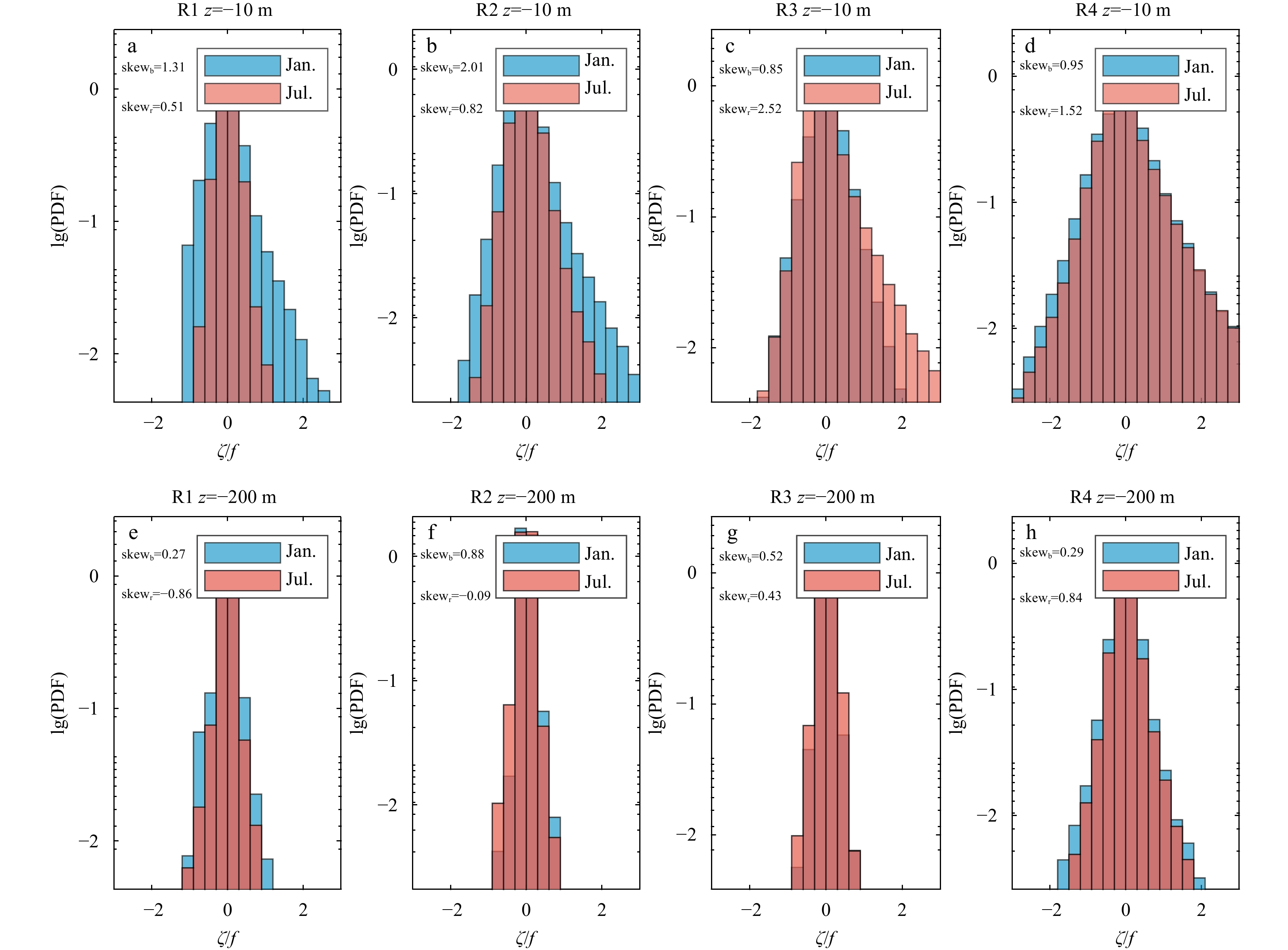
To further examine the features of submesoscale eddies, this section statistically compares the vertical vorticity on the selected winter and summer months (January versus July) in the four sub-regions. The distributions of the vertical vorticity show prominently seasonal differences at the near-surface layer of the northern regions (R1 and R2; Figs 6a, b), which are much less for the southern regions (R3 and R4; Figs 6c, d). In the northern regions (R1 and R2), there appear more energetic submesoscale eddies in winter than in summer. In Fig. 6a (R1), the distribution of $ \zeta /f $at z=−10 m is markedly asymmetric in winter (blue bars) with a positive skewness of 1.31 and becomes much symmetric in summer (red bars, skewness=0.51). Note that the $ \zeta /f $ values are mostly larger than −1, as the bound for centrifugal instability. Differently, the submesoscale eddies ($\left| {\text{ζ} /f} \right|$>1) in R3 tend to be more energetic in summer than in winter, likely due to the strong submesoscale behaviors driven near the summer filament. It is interesting that the vorticity fields of R4 show a number of negative values of absolute vorticity ($\text {ζ} + f < 0$) that are favorable for centrifugal instability, as a consequence of the small Coriolis parameter at low latitudes (R4). This can also account for the strong submesoscale eddies in R4. A whole comparison between the upper layer (z=−10 m) and the deeper layer (z=−200 m) shows that the vertical vorticity is strongly reduced at the −200 m layer and its distribution becomes more symmetric.

Figure  6.  Probability of density functions (PDF) of wintertime (blue) and summertime (red) normalized vertical vorticity ζ/f for four sub-regions at two depth levels (upper row, z=−10 m and bottom row, z=−200 m). The skewness for each region is also marked. The subscripts b and r are short for blue and red bars, respectively.

DownLoad: Full-Size Img PowerPoint

3.3 Ertel potential vorticity analysis

Figure 7 shows the near-surface (−10 m) Ertel PV and its sub-components in the interested sub-regions on January 15 and July 15 to investigate the generating mechanisms of submesoscale processes in the sub-regions. The Ertel PV is as follows:

Figure  7.  Comparison of the near-surface (z=−10 m) Ertel potential vorticity q and its sub-components in different seasons. The upper (lower) raw shows snapshots on January 15 (July 15). Three sections (S1, S2, and S3) in the wintertime R1 and R4 and in the summertime R3 were selected for analyzing the vertical distribution of Ertel potential vorticity.

DownLoad: Full-Size Img PowerPoint

where b_z is the vertical gradient of buoyancy, u_z is the vertical shear, and $ {\nabla _h}b $ is the horizontal gradient of buoyancy. As shown in Eq. (1), q_vert is primarily attributed to the absolute vorticity in the case of stratified flow (N²>0, where N is the buoyancy frequency), and q_bc is associated with the lateral buoyancy gradient and the vertical shear of flow velocity. The winter and summer Ertel PV fields both show pronounced spatial differences. In winter (upper row, Fig. 7), the q field in R1 tend to be negative (Fig. 7b) resulting from negative q_vert, likely due to surface cooling that may cause gravitational instability; while the q_bc presents filamentous positive values particularly along the mesoscale eddy ring (Fig. 7c), which indicates the strong submesoscale eddies. This is contrary to the paradigm of geostrophic balance that q_bc is anticipated to be negative in the northern hemisphere (Thomas et al., 2013) and can be considered as a signature of energetic ageostrophic motions. Submesoscale filamentous q_bc can also be detected in other sub-regions (Fig. 7c). In R1 and R2, the negative q fields are favorable for the generation of symmetric instability (Thomas et al., 2013; Brannigan, 2016). In contrast, the southern regions display positive q_vert presumably because they are less impacted by the winter monsoon with less heat loss at the surface (Fig. 7b). For example, in R4, the baroclinic component, q_bc, still dominates the Ertel PV field with the alternating positive-negative filaments (Fig. 7c). As the buoyancy gradient of R4 is relatively weak (Fig. 5a), the strong baroclinic effect is supposed to result from the enhanced vertical shear due to the complex bottom topography.

A similar spatial pattern is shown for the summer Ertel PV field (bottom row) except for the strong summer filament in R3. In summer, the near-surface Ertel PV of R1 is still dominated by the q_vert with negative values especially in the north. Since the summertime absolute vorticity is mostly positive (Fig. 6), the negative q_vert results from the negative stratification at the surface boundary presumably due to the wind stirring. The Ertel PV at the strong summer filament is primarily dominated by the baroclinic component with clear pairwise negative-positive elongated features (R3). This is because of the opposite buoyancy gradients at the two flanks of the cold filament. The northern flank tends to be unstable with the negative Ertel PV, displaying submesoscale frontal waves (Figs 2d and 7d, R3). The summer Ertel PV in R4 shows much weaker submesoscale features. All these results indicate the underlying submesoscale instabilities in the four sub-regions.

Further insight into the vertical profiles of Ertel PV is conducive to understanding the generating mechanisms of submesoscale processes (three typical sections marked in Figs 7a, d). Section 1 crosses the mesoscale anticyclonic eddy and exhibits negative Ertel PV in the mixed layer and in the core of the eddy. The Ertel PV with opposite signs to the Coriolis frequency for flows is favorable for the development of symmetric instability that can drive large vertical motions (Brannigan, 2016). The deepened pycnocline in the eddy core largely strengths the q_vert by the intensification of density stratification. Notice that the baroclinic component (q_bc) acts to balance the q_vert field particularly at the bowl-like base of the mixed layer (highlighted by the black solid rectangles in Fig. 8c), illustrating PV conservation. The Ertel PV in the shade of islands is reduced to negative values due to the strong anticyclone in q_vert (marked out in Fig. 8e), which could also easily drive submesoscale instabilities. This provides strong evidence for the dynamical regimes of submesoscale eddies in R4 (Fig. 6d). The cross-front vertical profile of the summer cold filament western SCS (S3) presents a clear baroclinic contribution to submesoscale instabilities at the northern flank (Fig. 8i), which can extend to the depth of −150 m.

Figure  8.  Vertical profiles of Ertel potential vorticity q and its sub-components for the three typical sections marked in Figs 7a and d. The contours indicate the isopycnals (kg/m³).

DownLoad: Full-Size Img PowerPoint

3.4 Annual cycle of submesoscale features

To understand the seasonal variation of submesoscale activities, Fig. 9 shows the time series of the normalized relative vorticity for each sub-region over the upper 200 m, with root-mean-squared (RMS) values characterizing its strength. The mixed layer depth is also plotted for reference. Here the MLD is defined as the shallowest depth where the density difference is 0.03 kg/m³ from the surface layer. The normalized vorticity, $ \zeta /f $, for R1 undergoes a clear seasonal cycle, larger in winter and smaller in summer (Fig. 9a). The high values of $ \zeta /f $ in R1 appear during the wintertime, mostly contained in the mixing layer, while the $ \zeta /f $ becomes much weaker in summer. The strong Kuroshio intrusion in winter can also generate strong eddy variability in this region (Nan et al., 2011b). The annual cycle of $ \zeta /f $ in R2 is similar to that in R1. However, the R2 region displays weaker wintertime vorticity but stronger summertime vorticity compared to R1 (Fig. 9b). The biggest difference between R1 and R2 is that the former is more impacted by the northwestern Pacific through the Luzon Strait while the latter would be more associated with the monsoon. In Fig. 9c, the western SCS (R3) shows more energetic vorticity in late summer and early autumn when the monsoon starts to reverse (the summer monsoon takes place discussed in the following section). This may result from the wind-driven regional circulation which displaces the summer cold filament off the coast (Xie et al., 2003). As show in Fig. 2d, there appear a population of submesoscale eddies in the flanks of the filament as a result of both barotropic and baroclinic instabilities. The eddy variability is weakened after December and reaches its minimum in May. In Fig. 9d, the southern SCS (R4) exhibits relatively high $ \zeta /f $ events almost over the whole year that extend to a deeper layer (−100 m). No clear seasonal variation is shown in this region presumably because submesoscale activities do not strongly depend on the seasonal forcing but are more likely generated in the form of topography wakes.

Figure  9.  Time series of the root-mean-squared values of normalized vertical vorticity ζ/f for R1 (a), R2 (b), R3 (c), and R4 (d) over the upper 200 m. The green lines indicate the averaged mixed layer depth for each sub-region.

DownLoad: Full-Size Img PowerPoint

The horizontal divergence for the sub-regions displays similar annual cycles with the vertical vorticity for the sub-regions (Fig. 10 compared to Fig. 9). Interestingly, the divergence has two peaks at the surface boundary layer and the base of the mixed layer. It is no doubt that the former indicates the generation submesoscale processes; while the latter is because the mixed layer base serves as the lower bound for mixed processes, especially for ageostrophic motions. In addition, restratification would also drive ageostrophic motions at the mixed-layer base. This also explains why it agree well with the seasonal variation of the mixed-layer depth. In the upper ocean, the submesoscales are highly correlated to the strain rate for all the sub-regions (Fig. 11), suggesting that strain-induced frontogenesis would be one significant mechanism for the submesoscale processes (McWilliams, 2017). As afore-mentioned, the strain is calculated using the original velocity that includes both geostrophic and ageostrophic effects.

Figure  10.  Time series of the root-mean-squared values of normalized horizontal divergence δ/f for R1 (a), R2 (b), R3 (c), and R4 (d) over the upper 200 m. The green lines indicate the averaged mixed layer depth for each sub-region.

DownLoad: Full-Size Img PowerPoint

Figure  11.  Time series of the root-mean-squared values of normalized strain rate S/f for R1 (a), R2 (b), R3 (c), and R4 (d) over the upper 200 m. The green lines indicate the averaged mixed layer depth for each sub-region.

DownLoad: Full-Size Img PowerPoint

The buoyancy gradient is most pronounced approximately at the base of the mixed layer and displays different seasonalities for the sub-regions. As shown in Fig. 12a (R1), the RMS values of $ \left| {\nabla b} \right| $ in R1 can be larger than 1×10⁻⁷ s⁻² and extend to the depth of −100 m in winter, while it is largely reduced and shows weak vertical extent in summer. A similar annual cycle is shown in R2 (Fig. 12b). Notice that the R2 region displays different seasonality between the mixed layer and the deeper layer (e.g., z=−10 m versus z=−150 m). Together with the seasonal variation of relative vorticity in R2 (Fig. 9b), the relatively strong vorticity and buoyancy gradient during spring and summer tend to be a signature of mesoscale flows before the summer monsoon (Chu et al., 2020). The R3 region shows a distinct seasonal cycle with clear intensification in late summer and autumn, roughly consistent with the local eddy variability (Fig. 9). Compared with the other sub-regions, the R4 shows smaller $ \left| {\nabla b} \right| $ almost over the whole year, although this region shows larger RMS $ \zeta /f $, $\text{δ} /f$, and $ S/f $. This can be considered as evidence that baroclinic buoyancy production is less important in R4 than in the other sub-regions.

Figure  12.  Time series of the root-mean-squared values of buoyancy gradient ${\left|\nabla {b}\right|} $ for R1 (a), R2 (b), R3 (c), and R4 (d) over the upper 200 m. The green lines indicate the averaged mixed layer depth for each sub-region.

DownLoad: Full-Size Img PowerPoint

3.5 Annual cycle of vertical velocity

The large vertical velocity, w, could be a proxy for submesoscale activities. However, it may be valid for the mixed layer but not completely true for the deeper layers. The enhanced w does not exactly match the decreased vertical vorticity below the mixed layer. This is confusing to understanding the submesoscale motions below the mixed layer. As investigated in recent studies (Su et al., 2020; Cao and Jing, 2022), the vertical velocity is strongly enhanced at high frequencies (>f) and high wavenumbers (>0.1 km⁻¹), which significantly contributes to the vertical transport of tracers even below the mixed layer, while they do not significantly contribute to energy conversion through barotropic or baroclinic processes (Cao et al., 2021). Within the mixed layer, the vertical velocity is believed to result from submesoscale processes (Mahadevan et al., 2010; Gula et al., 2014); while below the mixed layer, the larger w is likely associated with along-isopycnal motions, spontaneous internal waves, or frontogenesis. Here we only present the seasonal cycle of the large vertical velocity instead of the investigating the underlying dynamics. Interestingly, the sub-regions exhibit different annual cycles of RMS w (Fig. 13), implying the different seasonal modulations. In R1, the vertical velocity below the mixed layer reaches its maximum in late winter and early spring, which is about two months later than the timing of strongest submesoscale processes (Fig. 13a). The strongest w of R2 occurs much later than the strong mixed layer submesoscale processes during the wintertime (Fig. 13b). Although R2 is adjacent to R1 in the north, their vertical motions present different seasonal variations. Again, this suggests that there are totally different dynamical regimes for the submesoscale activities of R1 and R2. The R3 and R4 regions both show an enhancement of deeper-layer vertical velocity during autumn, likely arising from the strengthened circulation in the southern SCS (Zhu et al., 2019).

Figure  13.  Time series of the root-mean-squared values of vertical velocity w for R1 (a), R2 (b), R3 (c), and R4 (d) over the upper 200 m. The green lines indicate the averaged mixed layer depth for each sub-region.

DownLoad: Full-Size Img PowerPoint

4. Correlation analysis

The above section examined the spatial and seasonal differences of submesoscale-related variables but provides limited information about their dynamical relations. This section investigates the correlations between the variables to gain some clues to the following issues: the vertical relations for the variables, the role of MLD, the vertical extent of $ w $, and the relation between submesoscale activities and monsoon index.

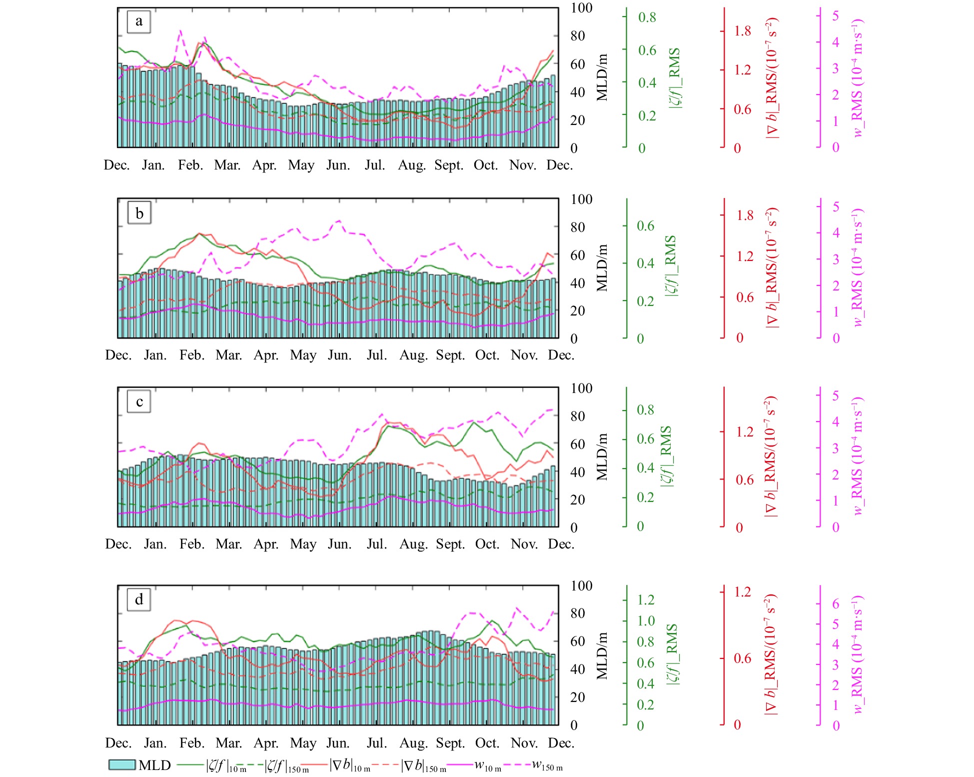
Figure 14 compares the seasonal cycles of RMS $ \left| {\zeta /f} \right| $ (green), $ \left| {\nabla b} \right| $ (red), and $ w $ (magenta) at two depth levels (solid lines for −10 m and dashed lines for −150 m, respectively). The MLD for each sub-region is also plotted for a correlation analysis. For most of the sub-regions, the 10-m $ \left| {\zeta /f} \right| $ and $ \left| {\nabla b} \right| $ experience a similar seasonal cycle, suggesting that the available potential energy is likely of great energy source for the submesoscale eddies through baroclinic processes in the mixed layer. At the −150 m layer (below the mixed layer), the submesoscale activities tend to be weakened and exhibit different seasonal cycles at the −10 m layer. In particular, the larger vertical velocity at the deeper layer shows more fluctuation over seasons.

Figure  14.  Time series of the root-mean-squared (RMS) $ \left| {\zeta /f} \right| $(green lines), $\left| {\nabla {b}} \right|$ (red lines), and w (magenta lines) for the sub-regions at the −10 m (solid lines) and −150 m (dashed lines) layer. The seasonal variation of mixed layer depth is indicated by the light blue bars.

DownLoad: Full-Size Img PowerPoint

To investigate the possible relations of submesoscale features in vertical, Table 1 lists the correlation coefficients of vertical vorticity, buoyancy gradient, and vertical velocity between the 10-m layer and 150-m layer for the four sub-regions. A better correlation between $\zeta /{f_{{\rm{RMS}},10}}$ and $ \zeta /{f_{{\text{RMS}},150}} $ is shown in R1 and R3, indicating a better vertical correspondence of eddies. Since submesoscale eddies are largely constrained in the mixed layer, the better vertical correspondence should result from mesoscale eddies in these two regions. This can also be verified by the correlation coefficients between the ${\left|\nabla {b}\right|}_{\text{RMS},10}$ and ${\left|\nabla {b}\right|}_{\text{RMS},150}$ (Table 1). The vertical velocity of the two depth levels correlates well only in R1, which again confirms the vertical extent of submesoscale features in this region. Table 2 shows the correlation coefficients of $\zeta /{f_{{\rm{RMS}}}}$ and $ {\left| {\nabla {{b}}} \right|_{{\text{RMS}}}} $ against the $ {w_{{\text{RMS}}}} $ for the two depths. The high correlation at the 10-m layer indicates that the vertical velocity predominantly arises from submesoscale processes. However, the correlation becomes weak at the 150-m layer, especially in R3 and R4. As mentioned above, the dynamical regime of vertical velocity below the mixed layer is complicated. The correlation between the MLD and the submesoscale characteristics at z=−10 m and is also examined (Table 3). The MLD is not so important to the upper ocean submesoscale activities except in R1.

Table  1.  Correlation coefficients of vertical vorticity, buoyancy gradient, and vertical velocity between the 10-m and 150-m layers for each sub-region. All the correlation coefficients passed the significance test within a confidence interval of 0.95 (p-value<0.05 indicates significant correlation)

Region	$\zeta /{f_{{\rm{RMS}},10} }$ vs. $ \zeta /{f_{{\text{RMS}},150}} $	$ {\left|\nabla {b}\right|}_{\text{RMS} ,10} $ vs. $ {\left|\nabla {b}\right|}_{\text{RMS} ,150} $	$ {w}_{\text{RMS} ,10} $ vs. $ {w_{{\text{RMS,}}150}} $
R1	0.87	0.84	0.78
R2	−0.24	−0.09	−0.45
R3	0.60	0.77	0.05
R4	−0.08	0.29	0.10

 | Show Table

DownLoad: CSV

Table  2.  Correlation coefficients between $ {w_{{\text{RMS}}}} $ and $\zeta /{f_{{\rm{RMS}}}}$, ${\left| {\nabla {b}} \right|_{{\text{RMS}}}}\;$ at z=−10 m and z=−150 m for each sub-region. All the correlation coefficients passed the significance test within a confidence interval of 0.95 (p-value<0.05 indicates significant correlation)

Region	$ {w_{{\text{RMS,}}10}} $ vs. $ \zeta /{f_{{\rm{RMS}},10}} $	$ {w_{{\text{RMS,}}10}} $ vs. $ {\left| {\nabla {{b}}} \right|_{{\text{RMS,}}10}} $	$ {w_{{\text{RMS,}}150}} $ vs. $ \zeta /{f_{{\text{RMS}},150}} $	$ {w_{{\text{RMS,}}150}} $ vs. $ {\left| {\nabla {{b}}} \right|_{{\text{RMS,}}150}} $
R1	0.98	0.97	0.84	0.88
R2	0.92	0.87	0.74	0.74
R3	0.68	0.87	0.85	0.55
R4	0.76	0.76	0.77	0.52

 | Show Table

DownLoad: CSV

Table  3.  Correlation coefficients between mixed layer depth (MLD) and $\zeta /{f_{{\rm{RMS}},10}}$, ${\left| {\nabla {b}} \right|_{{\text{RMS,}}10}}$, $ {w_{{\text{RMS,}}10}} $ for each sub-region. All the correlation coefficients passed the significance test within a confidence interval of 0.95 (p-value<0.05 indicates significant correlation)

Region	MLD vs. $ \zeta /{f_{{\rm{RMS}},10}} $	MLD vs. $ {\left| {\nabla {{b}}} \right|_{{\text{RMS,}}10}} $	MLD vs. $ {w_{{\text{RMS,}}10}} $
R1	0.84	0.72	0.83
R2	0.06	−0.20	0.26
R3	−0.50	−0.22	0.06
R4	0.04	−0.35	0.23

 | Show Table

DownLoad: CSV

The vertical extent of vertical velocity is investigated by examining the correlations of between vertical velocity at z=−5 m and that at other depth levels over the upper 200 m within each sub-region. In Fig. 15, higher correlation coefficients mean better vertical extent of vertical velocity driven by submesoscale mixed-layer activities—that is to say, if the high correlations can well extend to the deeper layer, submesoscale processes can directly transport tracers from the ocean interior to the near-surface layer in a short period; otherwise, the vertical motions may not be able to drive an effective vertical transport for the tracers even if the sub-surface vertical velocity is large (recall Fig. 13). The seasonal variation of the vertical extent is not exactly consistent with that of vertical vorticity particularly in R3 where there is no summer peak as in Fig. 9c. Further investigation suggests that the seasonal variation of vertical extent is dependent on the MLD (correlation coefficients between the white solid lines and MLD are estimated to be 0.92, 0.66, 0.70, and 0.81 for R1, R2, R3, and R4, respectively). It is the case that the mix-layer base is an important barrier for vertical transport between the mixed layer and the ocean interior.

Figure  15.  Time series of the correlation coefficients between vertical velocity at different depth levels and that at z=−5 m. For reference, the correlation coefficient of 0.5 is indicated by the white solid lines for each sub-region. All the correlation coefficients passed the significance test within a confidence interval of 0.95 (p-value<0.05 indicates significant correlation).

DownLoad: Full-Size Img PowerPoint

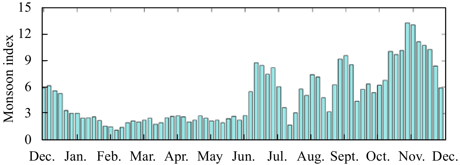
Since the SCS is strongly affected by the monsoon, the correlations between the SCS monsoon index (SCSMI) and vertical vorticity within each sub-region are further examined to investigate the wind effect on driving the submesoscale activities in the mixed layer. The wind may enhance the submesoscale flows directly by inputting negative potential vorticity or driving buoyancy flux (e.g., R2). Alternatively, the wind effect could indirectly affect the submesoscale flows by modulating the regional circulation or mesoscale flows (e.g., R3 where the summer cold filament occurs). Here we intend to investigate the relative importance of SCS monsoon to submesoscale flows for each sub-region. Figure 16 shows the summer monsoon index of the SCS calculated by meridional shear vorticity index (Wang et al., 2009) based on the daily wind data used for this simulation. The correlation coefficients between the SCSMI and $\zeta /{f_{{\rm{RMS}},10}}$, $ \zeta /{f_{{\text{RMS}},150}} $ for each sub-region are listed in Table 4. The R2 shows a relatively higher correlation coefficient between the SCSMI and $\zeta /{f_{{\rm{RMS}},10}}$ (R=−0.72; a negative correlation indicates the impact of winter monsoon), while the R3 has a better correlation between the SCSMI and $ \zeta /{f_{{\text{RMS}},150}} $ (R=0.75) compared to the other sub-regions. This suggests that the SCS monsoon may not be of great importance to driving the mixed-layer submesoscale activities except for R2, but in the southwestern region, the summer monsoon drives eastward offshore currents along 13°N and sometimes anticyclonic eddies off the southeast Vietnam coast (Zhu et al., 2019), indirectly resulting the strengthening of vertical vorticity during the summertime (recall Fig. 2d). Consequently, the correlation between SCSMI and vertical vorticity in R4 is also improved at the 150-m layer (R=0.53), although there is no clear seasonality of vertical vorticity in R4 (recall Fig. 9). Note that here we only examined the direct relationship between the SCSMI (defined by wind shear) and submesoscale processes. In effect, the monsoon may also affect the submesoscale processes indirectly by modulating the mesoscale flows and the MLD. More insightful work is required to investigate the underlying dynamical link between the monsoon and submesoscale processes in the SCS.

Figure  16.  Time series of the South China Sea monsoon index based on Wang et al. (2009).

DownLoad: Full-Size Img PowerPoint

Table  4.  Correlation coefficients between the South China Sea monsoon index (SCSMI) and $\zeta /{f_{{\rm{RMS}},10}}$, $ \zeta /{f_{{\text{RMS}},150}} $ for each sub-region

	R1	R2	R3	R4
SCSMI vs. $\zeta /{f_{{\rm{RMS}},10} }$	−0.33	−0.72	0.36	−0.17
SCSMI vs. $ \zeta /{f_{{\text{RMS}},150}} $	−0.21	−0.04	0.75	0.53

 | Show Table

DownLoad: CSV

5. Summary

This study investigates the seasonal and spatial differences of submesoscale activities in the upper ocean of the SCS by examining the seasonal variations of vertical velocity, horizontal divergence, strain rate, lateral buoyancy gradient, and vertical velocity from a high-resolution numerical simulation. Our results suggest that the submesoscale features in the sub-regions exhibit different seasonalities, attributed to different regimes as a result of the local circulation and forcing. The submesoscale activities in the northern SCS near the Luzon Strait (R1) are largely influenced by the loop flow shedding from Kuroshio as a consequence of the effect on mesoscale eddies (Zhang et al., 2020). In addition, this seems to be the only region where the development of submesoscale eddies is subject to the MLD (Table 3). Processes like mixed layer baroclinic instability are expected in this region (Fox-Kemper et al., 2008). The submesoscale processes in the SCS basin (R2) appear to be more related to the SCS winter monsoon, although its seasonal variation is similar to that of R1. In contrast, the western SCS (R3) displays totally distinct seasonal variation with stronger submesoscale behaviors in late summer. This is associated with the cold filament driven by the summer monsoon during that period, which can extend to the depth below the mixed layer. In R4, submesoscale processes are more like wake waves behind the islands and do not have clear seasonality.

However, more in-depth analyses are still required to understand the dynamical details in the southern regions as they are rarely investigated and have much larger geostrophic scale (smaller f). Besides, the enhanced vertical velocity below the mixed layer displays different seasonality from that within the mixed layer (e.g., R2, R4). The dynamical regimes for vertical velocity within the mixed layer should be the submesoscale activities, while the mechanism for the larger vertical velocity at the deeper layer remains unclear. More work is required to improve our understanding of the large vertical velocity, e.g., its time and space scales and dynamical mechanisms. This determines the vertical transport of oceanic tracers between the mixed layer and the ocean interior. In addition, this simulation with a resolution of ~1.5 km would resolve more submesoscale characteristics in the southern regions with lower latitudes and larger length scales for submesoscale processes (e.g., larger scales for ML baroclinic instability estimated by NH/f where H is the MLD, when f is smaller at low latitudes). So the resolution effect may affect the strength of simulated submesoscale features for different sub-regions but would not be concerned with their generating mechanisms.

Acknowledgements

We thank NASA (http://oceancolor.gsfc.nasa.gov) for the MODIS Aqua data and the QuikSCAT forcing (http://podaac.jpl.nasa.gov), NOAA ICOADS (http://icoads.noaa.gov), and SODA (https://www2.atmos.umd.edu/;ocean/) were also part of the forcing data.