Vertical multiple-layer structure of temperature and turbulent diffusivity in the South China Sea

1. Introduction

The South China Sea (SCS) covers a region from the equator to 23°N and from 99°E to 121°E with an average depth about 1 212 m. It is one of the largest tropical marginal seas on earth. It has a deep basin surrounded by a steep continental slope and connects to the East China Sea via the Taiwan Strait, to the western Pacific Ocean via the Luzon Strait, to the Sulu Sea via the Mindoro Strait, and to the Java Sea via the Karimata Strait.

A widely accepted notion is that the SCS has a unique, three-layer cyclonic-anticyclonic-cyclonic (CAC) circulation pattern. Upper-layer circulation in the SCS has been widely studied since the first report by Wyrtki (1961). The results of the Princeton Ocean Model suggests that seasonal upper-layer circulation patterns and upwelling phenomena are determined and forced by the wind, while the lateral boundary forcing plays a secondary role in determining the magnitude of circulation velocities (Chu et al., 1999). Principal component analysis of altimeter data shows that sea-level variation consists mainly of two modes, corresponding well to the first two modes of the wind stress curl. Mode 1 represents oscillation in the southern basin and shows little inter-annual variation, and Mode 2 represents weak oscillation in the southern basin and strong oscillation off the coast of central Vietnam (Shaw et al., 1999). It is thus concluded that, as a result of the seasonally reversed monsoon, upper circulation exhibits distinct seasonal variability with cyclonic circulation over the whole SCS basin in winter, cyclonic circulation in the northern half of the basin, and anticyclonic circulation in the southern half of the basin in summer (Hu et al., 2000; Liu et al., 2001; Su, 2004).

By contrast, middle- and deep-layer SCS circulation follows anticyclonic and cyclonic patterns, respectively (Lan et al., 2013). The results of a numerical experiment show that the basin circulation of the SCS is cyclonic gyres at the surface and in the abyss, but an anti-cyclonic gyre at intermediate depths (Yuan, 2002). This suggests that the SCS plays the role of a “mixing mill” that mixes the surface and deep waters to return them to the Luzon Strait at intermediate depths. An analysis of updated monthly climatology of observed temperature and salinity from the U.S. Navy Generalized Digital Environment Model revealed that basin-scale cyclonic circulation lies over the deep SCS, and that the boundary current transport of the cyclonic circulation is around 3.0×10⁶ m³/s, supporting speculation that the overflow of the Luzon Strait provides a source for the basin-scale deep SCS cyclonic gyre (Wang et al., 2011). Based on these studies, CAC circulation patterns in the upper, middle, and deep layers of the SCS have been suggested, although the depth range of each layer differs among studies (Gan et al., 2016).

A critical issue for understanding the vertical structure of circulation is the physical mechanism for maintaining the structure. Vertical motion induced by mixing is considered as the primary driving mechanism of the transformation of deep water in the deep SCS (Xie et al., 2013; Lan et al., 2013). By analyzing the potential density, potential vorticity, dissolved oxygen, and sediment distribution in the deep SCS, previous studies found that deep water in the SCS has similar characteristics to Pacific water at ~2000 m depth which implies that SCS deep water comes from deep northwestern Pacific via the Luzon Strait (Li and Qu, 2006; Qu et al., 2006). The enhanced diapycnal diffusivity in the SCS is about O(10⁻³ m²/s) below 1000 m and reaches O(10⁻² m²/s) in the Luzon Strait below 500 m (Tian et al., 2009). This suggests that intensified diapycnal mixing might be responsible for the transformation of deep water. Strong diffusivity in the SCS also enhances SCS water transformation by itself in the vertical direction (Shu et al., 2014). However, we still do not clearly understand the overall vertical structure of circulation and the physical mechanism for maintaining this vertical structure.

In this study, we revealed the vertical turbulence structure of the SCS and identify the depth range of each layer using the observed turbulent diffusivity ${\kappa }_{\rho } \left(z\right)$. Moreover, we distinguished the depth range of each layer using the root mean square of observed temperature fluctuations $\eta \left(z\right)$, which is an important indicator of turbulence.

The rest of the paper is organized as follows. In-situ data are introduced in Section 2. The depths of the water layers are presented in Section 3. Section 4 provides discussion of each water layer, and Section 5 offers conclusions.

2. Data

Figure 1 shows a sketch of the SCS landscape, together with the locations of the observation stations. The field data were measured using three different instruments: the Sea-Bird Electronic 911 Plus CTD, the Turbulence Ocean Microstructure Acquisition Profiler (TurboMAP, Wolk et al., 2002), and the Vertical Microstructure Profiler-Expendable (VMP-X, Shang et al., 2017b).

Figure  1.  Sketch of the measurement locations of local temperature and velocity shear in the SCS: Stas s1–s8 denote the locations of temperature data from CTD measurements along the section of 18°N; Stas q1–q5 are for the CTD data in the SCS central basin; Sta. kj1 is for the CTD data at the slope of the northern SCS; Stas c1–c9 are for the velocity shear data from VMP-X measurements with $ z $ up to 3900 m. Asterisks denote velocity shear data from TurboMAP measurements where $ z < 500\;\mathrm{m} $. Gray lines denote isobaths in meters.

DownLoad: Full-Size Img PowerPoint

At Stas c1–c9, we used VMP-X to measure the whole profile of turbulent velocity shear ($ \partial u/\partial z $) with depths up to 3900 m from cruises in September 2014 (Stas c7–c9) and April 2017 (Stas c1–c6), where u denotes horizontal velocity and z denotes depth. At other stations (marked by asterisks in Fig. 1), we used TurboMAP to measure 44 profiles of the velocity shear in the upper layer (z<500 m) from a cruise in April 2010. The data-sampling frequency of the sensors in the two profilers was 512 Hz and there were roughly 900 data points on average over a meter. From both TurboMAP and VMP-X measurements, we can estimate the viscous dissipation rate:

where $ \nu $ is the fluid kinematic viscosity and $\left\langle{\cdot}\right\rangle$ denotes a spatial average. From these measurements, we can also calculate the turbulent diffusivity (Osborn, 1980):

where $\varGamma$=0.2 is the mixing efficient and $ N $ is the buoyancy frequency. Using the same method, some of the results for the variations of ε and $ {\kappa }_{\rho } $ in space and time are reported by Shang et al. (2017a) and Liang et al. (2017). These studies demonstrated that $ {\kappa }_{\rho } $ measured with TurboMAP and VMP-X is reliable.

In addition to measurements of ($ \partial u/\partial z $) profiles, we also measured the profiles of temperature in the SCS (Fig. 2). Along the section of 18°N, we collected 37 temperature profiles at Stas s1–s8 from six scientific cruises (August 2007, May 2009, August 2012, March 2014, September 2016, and April 2017) (Fig. 2a). The measured depth was around 1500 m. These data sets are referred to as section temperature profiles. Stations q1–q5 were located in the basin area of the central SCS. We measured one temperature profile at each of the stations with measured depths up to 3900 m (Fig. 2b). These data sets were collected from a cruise in April 2017. They are referred to as basin temperature profiles. At the slope of the northern SCS, we collected 12 temperature profiles at Sta. kj1 from a cruise in November 2019 with measured depths up to 2000 m (Fig. 2c). These data sets are referred to as slope temperature profiles. All section, basin, and slope profiles were measured using the SeaBird Electronic 9-11 Plus CTD instrument. The data-sampling interval was 0.042 s and there were roughly 20 data points on average over a meter.

Figure  2.  Overview of vertical profiles of temperature in the section of 18°N (a), the central basin of the SCS (b), and the slope of the northern SCS (c).

DownLoad: Full-Size Img PowerPoint

3. Results

3.1 Turbulent diffusivity

Figure 3a shows the obtained $ {\kappa }_{\rho } $ as a function of $ z $ in double-logarithmic scales for $ z < 500\;\mathrm{m} $. There are 44 profiles of $ {\kappa }_{\rho }\left(z\right) $ at various locations covering most of the SCS area. Variations of $ {\kappa }_{\rho } $ in different horizontal locations are of an order of magnitude. With the limited data points at each $ z $, the calculated algebraic averages of $ {\kappa }_{\rho } $ for each vertical profile are not convergent.

Figure  3.  Measured $ {\kappa }_{\rho } \left(z\right) $ from 44 stations in the upper ocean (a) and direct kernel smoothing probability density distribution of the measured $ {\kappa }_{\rho } \left(z\right) $ in a for different values of $ z $ (b). The solid curve in a is the algebraic average value of $ {\kappa }_{\rho } $.

DownLoad: Full-Size Img PowerPoint

Figure 3b shows the evolution of the probability density function (PDF) $ P\left({\kappa }_{\rho }\right) $ with depth $ z $ in double-logarithmic scales. In the plot, the PDF data at each $ z $ were calculated from 44 data points with the direct kernel smoothing function. The sidebar shows the scale. We found that the probable values of $ {\kappa }_{\rho } $ for $ z > 80\;\mathrm{m} $ follow a power-law function of $ z $. Due to insufficient statistics, the data have large fluctuations that blur the scaling.

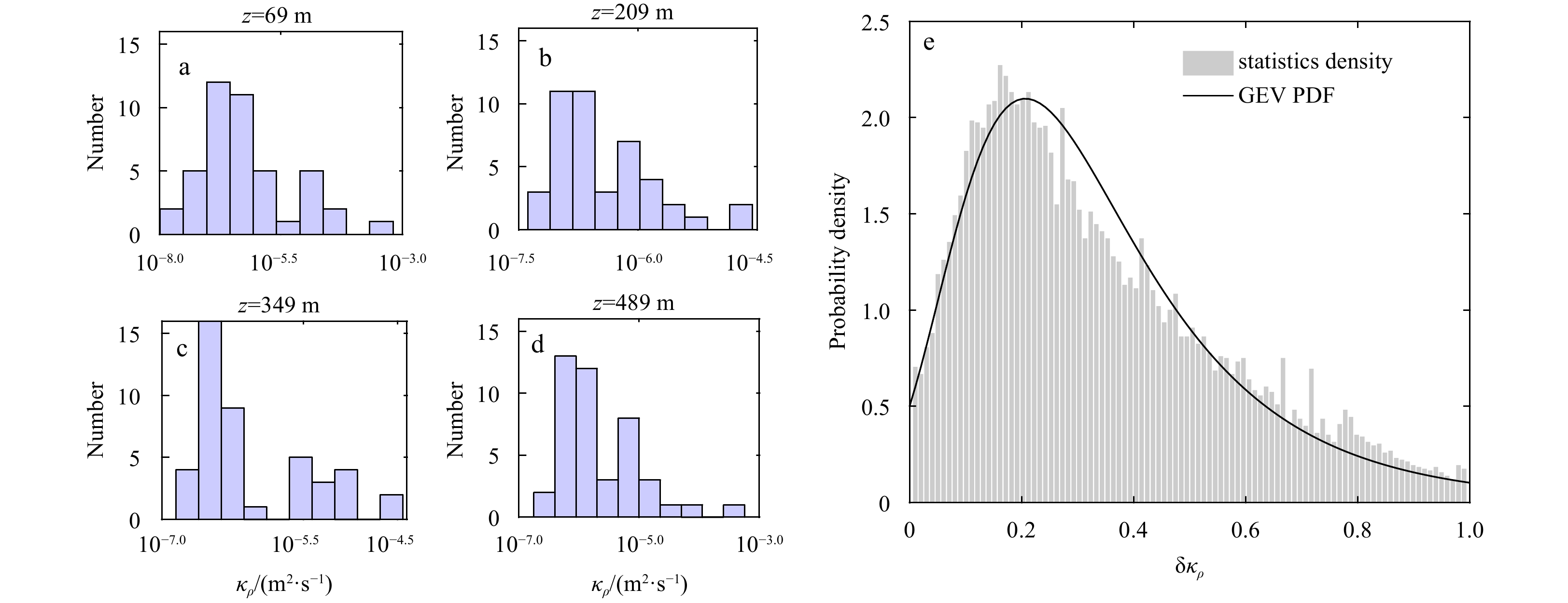
In order to improve the accuracy, we calculated the weighted average value of $ {\kappa }_{\rho } $, $ \left\langle{{\kappa }_{\rho }\left(z\right)}\right\rangle $, using the PDF as follows. For each depth, we calculate the dimensionless as follows:

where $ {\kappa }_{\max} $ and $ {\kappa }_{\min} $ are the maximal and minimal $ {\kappa }_{\rho } $, respectively. Figures 4a–d show the histogram of $ {\kappa }_{\rho } $ at several depths. These histograms have a similar distribution pattern. We assumed that the fluctuations of $ {\kappa }_{\rho } $ between the two extremes follow the same distribution, which is independent of depth. We collected all the ${\rm{\delta}} {\kappa }_{\rho }$ data from different z and show the PDF P(${\rm{\delta}} {\kappa }_{\rho }$) with ${\rm{\delta}} {\kappa }_{\rho }$ in Fig. 4e. The result indicates that P(${\rm{\delta}} {\kappa }_{\rho }$) follows a generalized extreme value (GEV) distribution with the following equation:

Figure  4.  Statistics of diffusivity in 10 segmentations of measured ranges at 69 m (a), 209 m (b), 349 m (c) and 489 m (d), and statistics density of diffusivity in 100 segmentations of measured ranges at all depths (e). The black solid curve in e shows the generalized extreme value (GEV) probability density function (PDF).

DownLoad: Full-Size Img PowerPoint

where $ \sigma $ is scale parameter, $ \mu $ is location parameter and $\text{γ}$ is shape parameter.

The GEV distribution is often used to model the smallest or largest value among a large set of independent, identically distributed random values representing measurements or observations. It indicates that each value of $ {\kappa }_{\rho } $, which is the average over a meter, is greatly influenced by the largest value of roughly 900 data points. Thus, we obtained the weighted average value of $ {\kappa }_{\rho } $ using the GEV distribution to illustrate the vertical turbulent structure in the SCS. Using all the dimensionless ${\rm{\delta}} {\kappa }_{\rho }$ data, the parameters for the GEV distribution were calculated by maximum likelihood estimates. The values of scale parameter $ \sigma $, location parameter $ \mu $, shape parameter $\text{γ}$ are 0.1763±0.0030, 0.2248±0.0039, 0.1099±0.0189 with 95% confidence intervals.

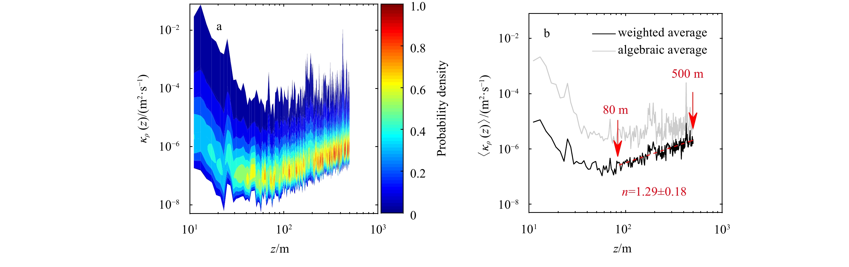
Figure 5a shows the probability density function (PDF) $P\left({{\rm{\delta}} \kappa }_{\rho }\right)$ with the depth z in double-logarithmic scales, and Fig. 5b shows a comparison between the algebraic average values and weighted average values $\left\langle{{\kappa }_{\rho } \left(z\right)}\right\rangle$ as a function of z. At depths above 40 m, known as the ocean surface mixed layer, the decreasing weighted average values $\left\langle{{\kappa }_{\rho } \left(z\right)}\right\rangle$ indicated that stratification is enhanced with increasing $ z $. In the range of 40 m<z<80 m, stratification is strongest, such that the weighted average values $\left\langle{{\kappa }_{\rho } \left(z\right)}\right\rangle$ reach the minimal value. We found that the vertical profile of the weighted average values $\left\langle{{\kappa }_{\rho } \left(z\right)}\right\rangle$ follows a power-law scaling $\left\langle{{\kappa }_{\rho } \left(z\right)}\right\rangle~{z}^{n}$ in the range of 80 m<z<500 m. As shown by the red solid line, a good fit with $ n = 1.29 \pm 0.18 $ is obtained for the spatial variations of $\langle {\kappa }_{\rho } \left(z\right)\rangle$.

Figure  5.  Generalized extreme value probability density distribution with $ z $ (a) and the algebraic average values and weighted average value $ \left\langle{{\kappa }_{\rho }\left(z\right)}\right\rangle $ with $ z $ (b). The red dotted curve is the fitting curve of the weighted average value for 80 m<z<500 m.

DownLoad: Full-Size Img PowerPoint

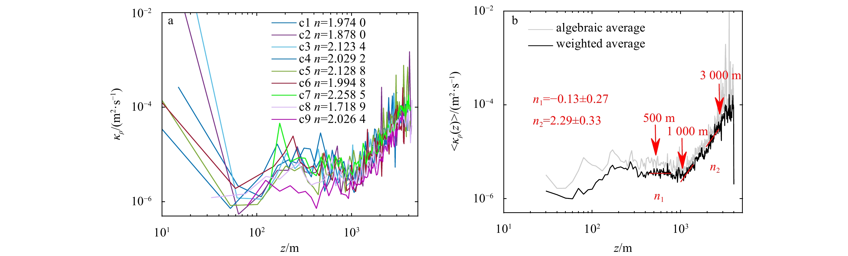
Figure 6a shows the vertical profile ${\kappa }_{\rho } \left(z\right)$ measured from the Stas c1–c9 with depths up to 3900 m. We calculated their weighted average values $\left\langle{{\kappa }_{\rho } \left(z\right)}\right\rangle$ using the same approach as described above, and we ploted $\left\langle{{\kappa }_{\rho } \left(z\right)}\right\rangle$ as a function of z as shown in Fig. 6b. The weighted average values are close to the algebraic averaged values below 1000 m because ${\kappa }_{\rho } \left(z\right)$ have similar order for all profiles. The profile $\left\langle{{\kappa }_{\rho } \left(z\right)}\right\rangle$ still reveals multiple scaling regimes with the power-law distribution $\left\langle{{\kappa }_{\rho } \left(z\right)}\right\rangle \sim {z}^{n}$. As indicated by the dashed lines in Fig. 6b, the power-law exponent n varies for different ranges of z. In the range of 500 m<z<1 000 m, $\left\langle{{\kappa }_{\rho } \left(z\right)}\right\rangle$ is almost independent of z and n$ = -0.13 \pm 0.27 $. For 1 000 m<z<3 000 m, a power-law fit to the data yields $ n = 2.29 \pm 0.33 $. At depths below 3000 m (except for the bottom boundary layer), $\left\langle{{\kappa }_{\rho } \left(z\right)}\right\rangle$ remains roughly 8×10⁻⁵ m²/s gradually. Stratification and flow are weak and stable in the deep SCS, so that any fluctuation leads to a large vary of $ {\kappa }_{\rho } $. Constant $ {\kappa }_{\rho } $ below 3000 m might be due to the effect of bottom topography.

Figure  6.  The profiles of $ {\kappa }_{\rho } $ and the $ n $ values of the power-law fit for 1 000 m<z<3 000 m from Stas c1–c9 (a) and the weighted average and algebraic average values of $ {\kappa }_{\rho } $ in a (b). The red dotted curves are the power-law fitting curves. n₁ and n₂ are the $ n $ values of the power-law $ \left\langle{{\kappa }_{\rho }\left(z\right)}\right\rangle\sim {z}^{n} $ from the weighted average $ {\kappa }_{\rho } $ profile for $ 500\;\mathrm{m} < z < 1\;000\;\mathrm{m} $ and $ 1\;000\;\mathrm{m} < z < 3\;000\;\mathrm{m} $, respectively.

DownLoad: Full-Size Img PowerPoint

3.2 Temperature

Similar multiple-layer scaling regimes are also observed from the root mean square of temperature fluctuation:

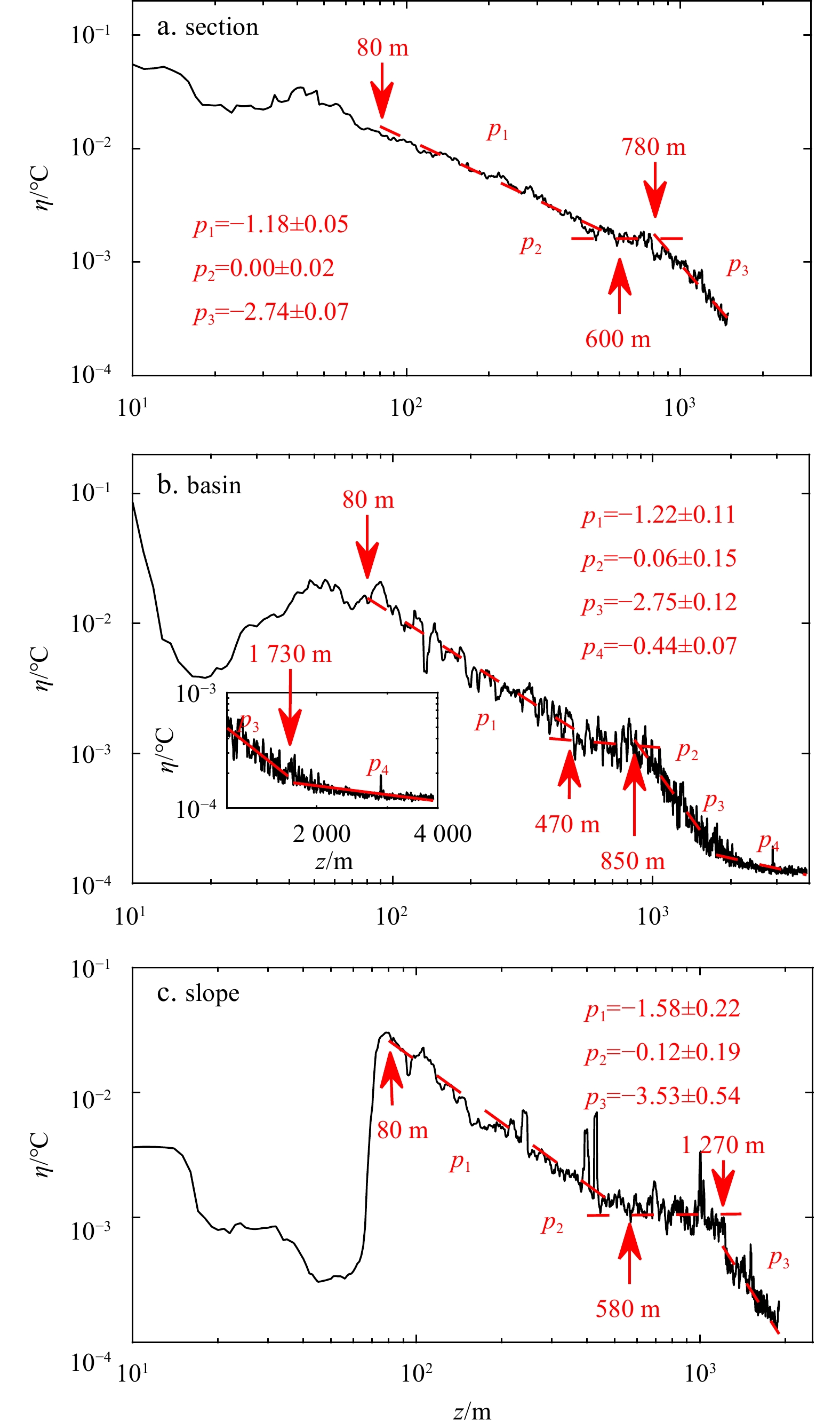
where $\bar{T}$ is the algebraic averaged value of a temperature dataset which have K elements, i=1, 2, ···, K, and $ {T}_{i} $ is the temperature of the i-th element. Figures 7a−c show the measured $ \eta \left(z\right) $ as a function of $ z $ in the section of 18°N, the basin area of the SCS, and the slope of the northern SCS, respectively. In each plot, the profile $ \eta \left(z\right) $ is obtained by averaging all the data points from different stations in the corresponding region. The measured $ \eta \left(z\right) $ follows a power-law scaling $\eta \left(z\right) \thicksim {z}^{p}$ with the exponent $ p $ varying at different layers. The separation depths $ {Z}_{{\rm{S}}} $ between two adjacent layers are determined by the intersect of the two power laws and are shown in Table 1. For convenience, we refer to these layers (from top to bottom) as the upper layer (UL), transition layer (TL), middle layer (ML), and deep layer (DL).

Figure  7.  Measured temperature root-mean-square profile $\eta \left(z\right)$ in the section of 18°N (a), the central basin of the SCS (b) and the slope of the northern SCS (c). The red dotted curves are the power-law fitting curves. The inset in b shows an expanded view of the profile for $z > 1\;200$ m. p₁, p₂, p₃ and p₄ are the $ p $ values of the power-law $\eta \left(z\right) \sim {z}^{p}$ in the upper layer, transition layer, middle layer, and deep layer, respectively.

DownLoad: Full-Size Img PowerPoint

Table  1.  Depth ranges of water layers

Area or source	ZS of water layer/m
	UL	TL	ML	DL
Section of 18°N	80−600	600−780	780 to NAN	NAN
Central basin in the SCS	65−470	470−850	850−1730	1730 to NAN
Slope of the northern SCS	80−580	580−1270	1270 to NAN	NAN
$ \left\langle{{\mathit{\kappa }}_{\mathit{\rho }}\left(\mathit{z}\right)}\right\rangle $	80−500	500−1000	1000 to NAN	NAN
Model (Gan et al., 2016)	0−750	NAN	750−1500	1500 to NAN
Note: NAN means no data. UL: upper layer, TL: transition layer, ML: middle layer, and DL: deep layer.

 | Show Table

DownLoad: CSV

The measured $ \eta \left(z\right) $ follows power-law scaling below 80 m where the weighted average values of $ {\kappa }_{\rho } $ follows a power law $\left\langle{{\kappa }_{\rho } \left(z\right)}\right\rangle \propto {z}^{n}$. ULs mainly occupy at depths of 100–500 m, in which $\eta \left(z\right)$ follows power-law scaling $\eta \left(z\right) \sim {z}^{p}$, where $ p $ is approximately –1.2. The starting depth of TLs is roughly 500 m. In the TLs, $\eta \left(z\right)$ is almost independent of z, and $ p $ is approximately equal to zero, which differs from that in the ULs and MLs. Further, $\eta \left(z\right)$ in MLs follows power-law scaling $\eta \left(z\right) \sim {z}^{p}$ with $p = -2.74$, $p = -2.75$, and $p = -3.53$ in the section, basin, and slope, respectively. Due to insufficient deep ocean temperature data, the DL is only found in the basin where $ \eta \left(z\right) $ follows power-law scaling with $ p = -0.44 $. Except for TL, the depth ranges of the multiple-layer structure agree with the model results byGan et al. (2016), namely, the upper layer (<750 m), middle layer (750−1 500 m), and deep layer (>1 500 m). TL is located between the UL and ML. It might play an important role in the exchange of energy and momentum between the UL and ML. Furthermore, these observations suggest that power-law scaling of $\left\langle{{\kappa }_{\rho } \left(z\right)}\right\rangle$ and $\eta \left(z\right)$ can be used to identify the multiple-layer structure of the SCS. With this method, a three-dimensional multi-layer structure of the SCS can be portrayed with sufficient temperature data or turbulence data.

4. Discussion

4.1 Transition layer

Through in-situ turbulence and temperature data, we revealed the multiple-layer structure of the SCS. The results prompt more questions, however, especially regarding the TL, which to our knowledge has not been mentioned in earlier studies.

The salient feature of TL is that $ n = 0 $ and $ p = 0 $ in power-law scaling of $\left\langle{{\kappa }_{\rho } \left(z\right)}\right\rangle$ and $\eta \left(z\right)$. One parameter is important for ocean temperature profile, the turbulent thermal diffusivity $ {\kappa }_{t} $, defined as

where $ {\left\langle{\cdot }\right\rangle}_{t} $ denotes a long time average, and $v'$ and $\theta '$ denote fluctuations of velocity and temperature, respectively. In oceans, it is often assumed that $ {\kappa }_{t} = {\kappa }_{\rho } $ (Thorpe, 2005), because density variations are predominantly caused by temperature variations. Therefore, we discuss the scaling behavior of the measured $ {\kappa }_{\rho } $, assuming that the obtained exponent $ n $ is the same as that for $ {\kappa }_{t} $. Munk (1966) explored the consequences of uniform upwelling ($ {w}_{0} $) over the entire abyssal ocean. He assumed a one-dimensional temperature advection/diffusion balance of the following form:

with constants $ {w}_{0} $ and $ {\kappa }_{t} $. The solution is

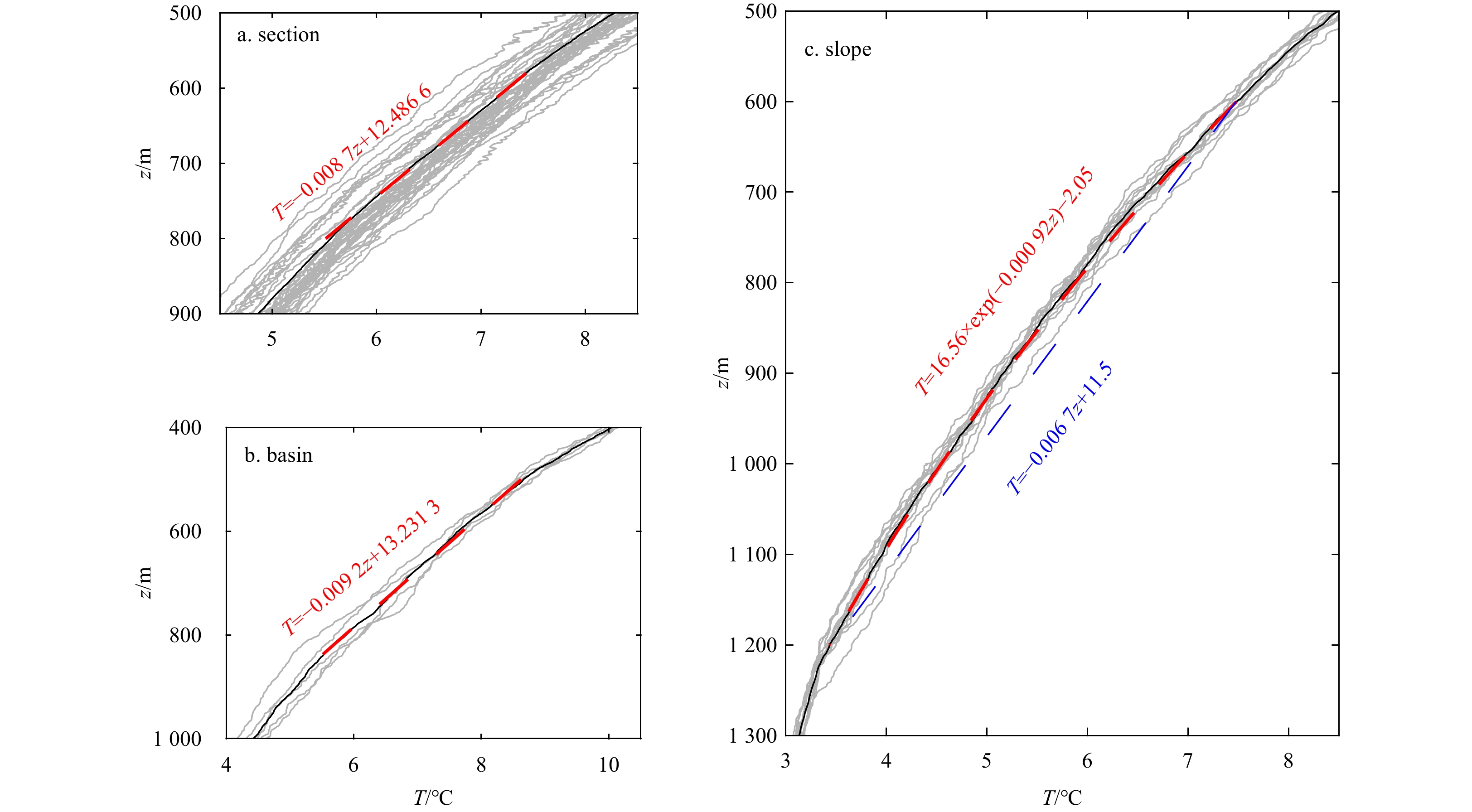
Figures 8a–c show the temperature profiles $T \left(z\right)$ and their fitted curves in the TL. The profiles $T \left(z\right)$ change approximately linearly with $ z $ in the section and basin, indicating that $T \sim z$ and ${w}_{0} = 0$. The downward transfer of heat is laminar without the vertical velocity and the vertical gradient of turbulent temperature diffusivity. Thus, temperature fluctuations that come from the upper ocean are obstructed at around 500 m.

Figure  8.  Measured temperature profiles (grey curves), averaged temperature profile (black curve), and fitting temperature profile of the transition layer (red dotted line) in the section of 18°N (a), the central basin in the SCS (b), and the slope of the northern SCS (c), respectively. The blue dotted line is the linear fitting temperature profile of the transition layer in slope.

DownLoad: Full-Size Img PowerPoint

The thickness of the TL is roughly 300 m and the current in the TL is weak in these areas where the sea bottom topography is smooth. As such, it was difficult to distinguish the TL in the earlier studies. Now, we can distinguish the TL by the root mean square of temperature fluctuations $\eta \left(z\right)$ and obtain the spatial distribution of the TL in the SCS with sufficient temperature data. Yet, the dynamic mechanism of the TL requires sufficient velocity data.

Only in the slope, the profile $T \left(z\right)$ shows ${\kappa }_{t}/{w}_{0} = 1\;087$ m and the TL is much thicker. We assume that the steep continental slope plays an important role in this phenomenon. The slope give rise to a vertical velocity. This suggests that temperature fluctuations from the upper ocean can be transferred deeper and temperature profile shows exponential form in TL. In contrast, the vertical velocities of most of smooth areas are negligible, corresponding to linear temperature profiles in TL of section and basin. Considering a common structure is showed in $ {\kappa }_{\rho } $ profiles, the temperature profile should also have a common function in other layers. We discuss the common function below.

4.2 Self-similarity function

Kitaigorodskii and Miropolskii (1970) were the first to describe the vertical temperature structure of an active oceanic layer by means of a self-similarity function that can be expressed as the functional dependence between the dimensionless temperature and depth as follows:

where $ {h}_{S} $ is the depth of the upper boundary of the water layer, $ {h}_{D} $ is the depth of the lower boundary of the water layer, $ {T}_{S} $ is the temperature of $ {h}_{S} $, and $ {T}_{D} $ is the temperature of $ {h}_{D} $. Golosov et al. (2018) proposed that the self-similarity representation of the vertical temperature profile indicates the constancy of the vertical gradient of temperature at any point of the considered profile.

In earlier studies that only considered the self-similarity function of the active oceanic layer, the conception of multiple layers was not acknowledged. To eliminate the effect of multiple layers, we calculate the dimensionless temperature $ \theta $ and dimensionless depth $ \xi $ by $\theta = \dfrac{{T}_{S} - T}{\Delta T}\;\mathrm{a}\mathrm{n}\mathrm{d}\;\xi = \dfrac{z - {h}_{S}}{{L}_{\lambda }}$, while ${L}_{\lambda } = \dfrac{\Delta T}{\dfrac{\partial }{\partial {z}}{\left.T\right|}_{z={h}_{S}}}$ at $ {h}_{S} \leqslant z $. Thus, the self-similarity function of each layer only has one adjusted parameter $ \Delta T $, where as $ {L}_{\lambda } $ depends on the starting depth and $ \Delta T $ (Table 2).

Table  2.  Adjusted parameters for each layer

Region	Water layer	Parameter
		$ \Delta \mathit{T} $/°C	$ {\mathit{L}}_{\mathit{\lambda }} $/m
Section of 18°N	UL	26.9	330
	ML	4.4	618
Central basin in the SCS	UL	27.8	234
	ML	3.8	541
Slope of the northern SCS	DL	0.5	645
	UL	29.8	175
	ML	0.9	394

 | Show Table

DownLoad: CSV

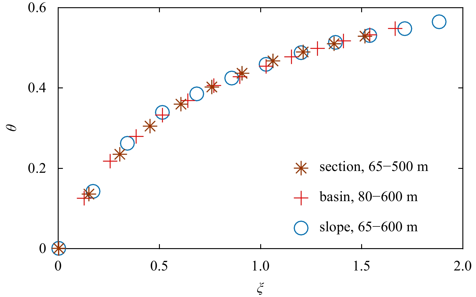
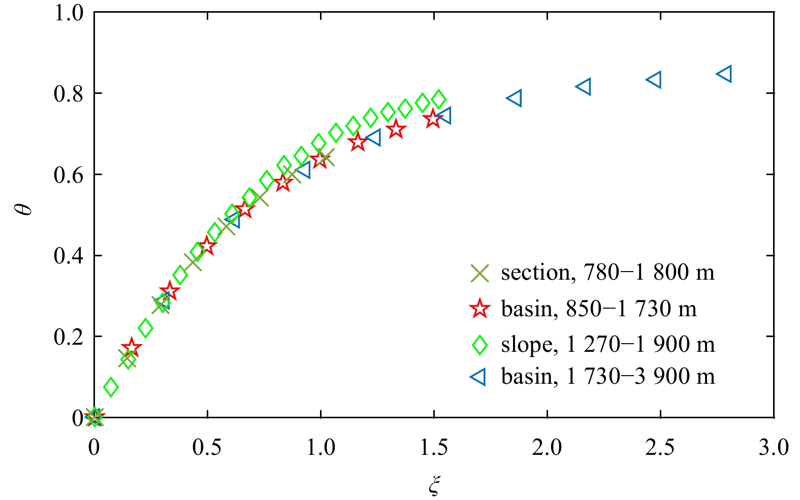
Figures 9 and 10 show the $ \theta $ with the $ \xi $ of each layer at explicit depths. The overlapping curves indicate that dimensionless temperature profiles $\theta \left(\xi \right)$ have a same self-similarity function in corresponding water layers, but with different parameters in different areas. Because the stratification is influenced by the surface layer, the self-similarity function of UL is markedly different from the function of ML.

Figure  9.  Dimensionless temperature profiles of upper layer in the section of 18°N, the central basin in the SCS, and the slope of the northern SCS.

DownLoad: Full-Size Img PowerPoint

Figure  10.  Dimensionless temperature profiles of middle layer in the section, basin, slope, and deep layer in the basin.

DownLoad: Full-Size Img PowerPoint

Interestingly, the function of the basin DL is consistent with the function of ML, but the function of the slope ML is slightly different. In the ML of the slope, the temperature profile can be affected by strong bottom friction from the steep continental slope. Moreover, there is no more external influence in the DL of basin, as with the ML of the basin and section. This might also be the reason that turbulent diffusivity $\left\langle{{\kappa }_{\rho } \left(z\right)}\right\rangle$ cannot clearly distinguish the ML and DL. It indicates that distribution of $ {\kappa }_{\rho } $ could not be used as an indicator of the vertical structure of the circulation solely.

Thus, we proposed that there is one constant function of the dimensionless temperature profile in water layers that have identical turbulence conditions. The rough bottom topography affects the turbulence of the entire water layer. In future studies, the distribution of adjusted parameters can be obtained from abundant temperature data, which will help us to understanding the structure of circulation in the SCS more explicitly.

5. Conclusions

Using observations, we identified the multiple-layer structure of the SCS to better understand its circulation pattern. In earlier studies, the vertical structure of circulation was explored from velocity field, although this is challenging with field measurements of the real ocean (Tian et al., 2006, 2009; Lan et al., 2013; Gan et al., 2016). In this study, $ {\kappa }_{\rho } $ was used to identify turbulence conditions of layers, and temperature fluctuations were used to identify the depth ranges of layers. Combining $ {\kappa }_{\rho } $ and temperature fluctuations, the vertical structure of temperature was revealed. We found that turbulence conditions were identical in the ML and DL without external fluctuations. Based on temperature profiles, the constant dimensionless temperature functions of each layer were verified. These dimensionless functions are dominated by turbulence conditions, except for the function dominated by the vertical velocity in TL where turbulent diffusivity is constant.

Our study of the multiple-layer structure provides a further improvement over previous theoretical methods. The solution of the temperature profile by Munk (1966) is useful for calculating the vertical velocity of real ocean areas, like steep continental slopes, which have a thick transition layer with constant turbulent diffusivity. Furthermore, the self-similarity function provides a profitable tool for supervising turbulence exclusively using a dimensionless temperature profile.

Considering the inadequate observations, more research is needed to verify our conclusions. Although this was a preliminary study, it improves our understanding of the vertical multiple-layer structure of the SCS. In particular, it will be crucial for exploring the physical mechanism for maintaining the temperature structure.