Figure
1.
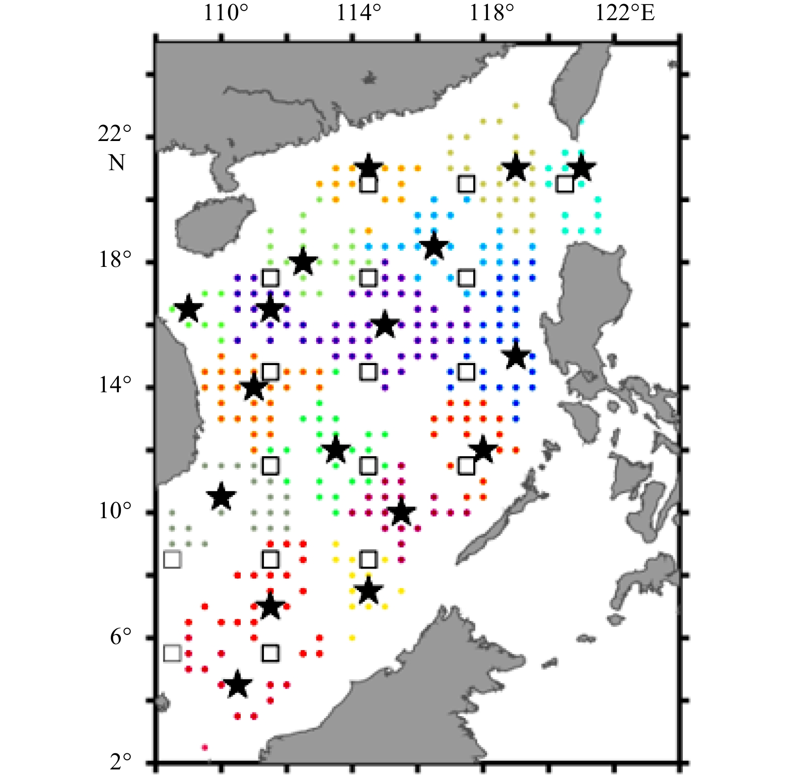
Topography of the South China Sea. White squares represent the locations of the assumed initial array.
| Citation: | Mengxue Qu, Zexun Wei, Yanfeng Wang, Yonggang Wang, Tengfei Xu. Objective array design for three-dimensional temperature and salinity observation: Application to the South China Sea[J]. Acta Oceanologica Sinica, 2022, 41(7): 65-77. doi: 10.1007/s13131-021-1975-z

|
Oceanography depends on observations. Accurate and sufficient observations are the essential prerequisites for revealing ocean phenomena, understanding ocean variability, and improving ocean prediction skills. The continuous measurement of ocean variables at fixed stations, such as a moored buoy array or subsurface mooring array (collectively referred to as moored or mooring array hereafter), is one of the most important approaches to collect long-term time series of the three-dimensional data on ocean temperature, salinity, and velocity. Although the ideal number of moored array sites is “the more the better”, available sites, however, could never be adequate to cover the investigated domain due to costly instruments required for each site in reality. Therefore, it is important to determine the optimum array design using a limited number of station sites. The site locations in an optimum array design should be the most “representative” of the area of interest and would thus yield the best estimation or prediction of oceanic characteristics (Lermusiaux, 2007; Zhang et al., 2020).
One way of determining an optimum array design is by conducting an observation system simulation experiment (OSSE) (Masutani et al., 2010). The OSSE approach was first used in the meteorological community to assess potential improvements in numerical weather prediction with additional observations involved and was later widely used to design the meteorological station network (Arnold and Dey, 1986). The application of OSSEs in physical oceanography has been promoted by an increase in ocean observation. Examples include optimal designs of a tide gauge array (McIntosh, 1987), tropical Atlantic mooring array (Hackert et al., 1998), monitoring array for the North Atlantic meridional overturning (Hirschi et al., 2003), tropical Indian Ocean mooring array (Ballabrera-Poy et al., 2007; Oke and Schiller, 2007; Sakov and Oke, 2008), Pacific Ocean mooring array (Zhang and Bellingham, 2008; Liu et al., 2018b), and mooring arrays for regional and coastal seas (Frolov et al., 2008; Yildirim et al., 2009; Fu et al., 2011; Xue et al., 2011; Zhang et al., 2019; Geng et al., 2020). The OSSEs have also been employed to assess the ability of a moorings observing system in monitoring the intraseasonal variability of currents in the northwestern tropical Pacific Ocean (Liu et al., 2018a). In addition, several investigations have used OSSEs to propose an optimum sampling design for hybrid instruments and platforms, e.g., glider-mooring observing system (Alvarez and Mourre, 2012) and Argo-mooring observing system (Gasparin et al., 2015).
A moored array design is essentially an optimization problem to identify optimal observation locations under constrained conditions. The most commonly used methods for qualifying the effectiveness of an array fall into three classes: (1) numerical modeling with data assimilation schemes (Fujii et al., 2019; Zhang et al., 2020), (2) conditional nonlinear optimal perturbation (CNOP) or singular vector (SV)-based targeted observation (Palmer et al., 1998; Zhang et al., 2020), and (3) empirical orthogonal function (EOF)-based determination of the best observing locations (Oke and Schiller, 2007; Zhang and Bellingham, 2008). Data assimilation can significantly improve the simulation capability of an ocean model by assimilating observational data into the model to reduce biases between the simulated and observed ocean. Its advantage for the design of an optimum observation system lies in the fact that it directly contributes to improving ocean simulation and prediction. The data assimilation-based approach has been successfully applied to both open and coastal oceans (Ballabrera-Poy et al., 2007; Vecchi and Harrison, 2007; Sakov and Oke, 2008; Fu et al., 2011; Oke and Sakov, 2012; Liu et al., 2018a, 2018b; Fujii et al., 2019; Geng et al., 2020). The disadvantage of the data assimilation-based approach is that its huge computation needs require a High-Performance Computing Cluster (HPCC). Therefore, it is not possible to perform this analysis on personal computers or workstations, and it is also difficult to switch between different HPCC platforms. The SV- or CNOP-based approaches seek optimal observation locations based on the fastest growth of initial errors in a forecast model (Mu and Duan, 2003). The CNOP-based approach has been demonstrated to be effective for improving predictions of ocean-atmospheric phenomena, such as the El Niño-Southern Oscillation, Indian Ocean Dipole, and Kuroshio variability (Hu and Duan, 2016; Feng et al., 2017; Zhang et al., 2017, 2019).
In addition to the data assimilation and CNOP approaches, both of which use numerical modeling and therefore require HPCC support, the EOF-based approach provides a simple and economic approach for optimum array design (Oke and Schiller, 2007; Zhang and Bellingham, 2008). An EOF analysis can decompose an ocean field into a set of spatial modes weighted by corresponding time series coefficients (Thomson and Emery, 2014). Hence the ocean field can be reconstructed by the superposition of several leading modes, with the reconstruction error determined by the number and accuracy of these modes and their amplitudes. The optimum array is then identified by picking the locations that yield the smallest reconstruction error. An EOF analysis resolves only individual two-dimensional variables. Consequently, the optimum arrays for ocean temperature and salinity at different depths are inconsistent with each other. Therefore, it needs an appropriate method to consolidate these arrays as vertically consistent, which has not been fully addressed yet.
The South China Sea (SCS), the largest semi-enclosed marginal sea in the Northwest Pacific Ocean, has multi-scale dynamic processes (Hu et al., 2020). Researchers have built and continue to maintain long-term continuous observation stations in the SCS. The Ocean University of China (OUC) has maintained a moored array in the northeastern SCS since 2009. This array has successfully captured ocean dynamic processes such as Luzon Strait transport and deep currents (Yang et al., 2007; Zhang et al., 2015; Zhao et al., 2014), Kuroshio loop current (Sun et al., 2020), deep west boundary current (Zhou et al., 2017), as well as mesoscale eddies, internal waves, and internal tides (Huang et al., 2017, 2018; Wang et al., 2020). The South China Sea Institute of Oceanology, Chinese Academy of Sciences has organized an annual series of scientific open cruises with the goal of establishing a mesoscale hydrological and marine meteorological observation network in the SCS (Yang et al., 2015; Zeng et al., 2015). The First Institute of Oceanography, Ministry of Natural Resources has conducted a 10-year observation in the Karimata Strait focused on the SCS-Indonesian seas water exchange and its impacts on seasonal fish migration (Wei et al., 2019). The moored arrays of these observation networks, however, focus more on specific scientific issues, and thus the distribution of these arrays is concentered in the northeastern SCS and in the Luzon and Karimata straits. The overall coverage is still rare, resulting in gaps in understanding and prediction of the three-dimensional SCS. Li et al. (2014) suggested that the SCS western boundary current (SCSWBC) region is a potential target observation area to improve forecast skill of ocean model over the SCS. Using an ensemble-based data assimilation method, Geng et al. (2020) suggested that the OUC arrays might oversample at the northwest of Luzon Strait and undersample at the northwest of Luzon Island. Their proposed optimal array provides better coverage in the northern SCS than the OUC arrays.
Currently, there are few investigations on how to design an efficient and economical array that is capable of detecting the dominant modes of basin scale variability in the SCS. In this study, we develop a moored array optimization tool (MAOT) that combines the EOF-based approach with a K-center clustering algorithm. The MAOT procedure has two steps: (1) derive optimal arrays of different variables at different depths using an EOF-based approach following Oke and Schiller (2007), and (2) consolidate these arrays using a K-center clustering algorithm. The MAOT is then applied to derive the optimum array for three-dimensional temperature and salinity observations in the SCS. It should be noted that we focus on variability at an interannual time scale for simplicity, but the MAOT could consider multi-scale variability.
The paper is organized as follows: Section 2 describes the data and methods, the results from a series of experiments are presented in Section 3, followed by a summary in Section 4.
The global reanalysis product Simple Ocean Data Assimilation (SODA) version 3.4.1 was used to provide three-dimensional temperature and salinity data on a monthly time interval from January 1980 to December 2015. The SODA3.4.1 is based on the Modular Ocean Model version 5 with optimum interpolation assimilation method being applied. The ocean model is forced by ERA-Interim near-surface atmospheric variables. Flux correction was applied to improve net surface heat and freshwater flux. The product covers the domain of 75.25°S–89.25°N, 0.25°E–179.75°W with a horizontal grid resolution of 0.5°×0.5° at 50 vertical levels. In the vertical dimension, the grid resolution changes from 10 m in the upper 100 m to much coarser resolution of around 250 m in the deep ocean. A detailed description of the SODA3 re-analysis can be found in Carton et al. (2018).
The SODA re-analysis data have been suggested in good agreement with Argo and in situ observations (Liang et al., 2019; Xiao et al., 2019). In addition, there are also lots of studies based on the SODA data, showing reasonable results of the meridional overturning circulation in the South China Sea, inter-basin transport through the Luzon, Mindoro and Karimata straits, and thermocline variability, etc. (Zhu et al., 2016; Peng et al., 2018). The EOF results of sea surface temperature based on SODA generally coincide with that of observations (Fang et al., 2006). Therefore, the SODA data is basically reliable, albeit may not fully capture all dynamical processes in the SCS.
It should be noted that there may be data-dependent for the MAOT approach, say, the optimal arrays would not necessarily consistent with each other based on different reanalysis products. In fact, the MAOT could give a consolidated array by considering multi-datasets with multi-variables, which would be better in terms of “ensemble mean” viewpoint. In this study, the key point is to show the application of MAOT in objective array design, therefore, for simplicity, we only use SODA data as an example.
The dominant EOFs of the variables could be used as a set of basic functions.
For a time series of two-dimensional variable such as temperature or salinity at each depth, it can be represented as
| $$ {w}^{a}=\overline{w}+{\boldsymbol{M}}c , $$ | (1) |
where
| $$ {\boldsymbol{M}}=\left[{w}_{1}^{\mathrm{E}\mathrm{O}\mathrm{F}},\ {w}_{2}^{\mathrm{E}\mathrm{O}\mathrm{F}},\ \dots,\ {w}_{m}^{\mathrm{E}\mathrm{O}\mathrm{F}}\right] , $$ | (2) |
where
The coefficients
| $$ H{\boldsymbol{M}}c={w}^{o} , $$ | (3) |
where
The accuracy of
The EOF-based optimum arrays contain temperature and salinity observations that are inconsistent with each other at different depths. Therefore, it is necessary to consolidate these arrays with consistent station locations at all depths. In previous studies, the most frequently occurring locations were selected for the consolidated array. This method is highly dependent on the horizontal grid resolution. In this study, the K-center clustering algorithm, which classifies similar elements into closely related clusters, is used to consolidate these arrays. The K-center clustering algorithm is adopted from Park and Jun (2009).
Suppose that N points should be grouped into K(K<N) clusters. In this study, the K values are determined as the proposed station numbers. The steps of K-center clustering algorithm are as follows:
(1) Initialize the K-center points by randomly select K points as the initial center of each cluster.
(2) Classify N points to K clusters. Firstly, the Manhattan distance is used as a dissimilarity measure in this study. The Manhattan distance between point i and j is given by
| $$ {{d}}\left(i,j\right)=\left|{x}_{i}-{x}_{j}\right|+\left|{y}_{i}-{y}_{j}\right| . $$ | (4) |
Secondly, the N points are classified as K clusters by assigning each point to the nearest initial center.
(3) Update the locations of the K-center points. In each cluster, the Manhattan distance for each point between the rest of points are calculated with their summation defined as total distance. The new locations of the K-center points are then selected as those yield minimum total distances.
(4) Repeat steps (2) and (3) until the change in minimum total distance for each of the K clusters is smaller than 10−4 m, and then these K-center points is regarded as the final locations.
In this study, the temperature and salinity compiled on the 0.5°×0.5° by 50 vertical levels from the SODA3.4.1 re-analysis product are assumed as the observed real fields. The procedure of MAOT for optimal array derivation contains the following steps: (1) starting with an array that includes all of the grid point of the analysis field in the SCS (a total of 673 points at 0.5°×0.5° resolution in this study); (2) excluding a single point which results in the smallest condition number of
The root mean square error (RMSE) between reconstructed and observed real field data is used to assess the observing ability of the initial, optimal, and consolidated arrays. The RMSEs at different depths are calculated as
| $$ {\rm{RMSE}}=\sqrt{\frac{1}{n}\sum _{i=1}^{n}{\left|{y}_{i}-{y}_{i}^{a}\right|}^{2}} , $$ | (5) |
where n is the number of grid points;
Since the temperature varies from around 30°C in the mixed layer to only 2°C in the deep layer, the RMSEs are also larger in the upper layers and smaller in the deeper layers. Therefore, the smaller RMSEs at depths do not necessarily mean that there is better observing ability in the deeper layers than in the upper layers. The averaged RMSEs (after area weighting) were divided by the ranges (the maximum minus the minimum) to obtain normalized RMSEs (NRMSEs). These are used to compare the improvement of the observing ability.
The optimization efficiency of array 2 relative to array 1 is defined as
| $$ {\rm{OE}}=\frac{\left({\rm{NRMSE1}}\;-{\rm{NRMSE2}}\right)}{{\rm{NRMSE}}1}\times 100\% , $$ | (6) |
where NRMSE1 is the NRMSE for the OSSE using array 1, and NRMSE2 is the NRMSE for the OSSE using array 2.
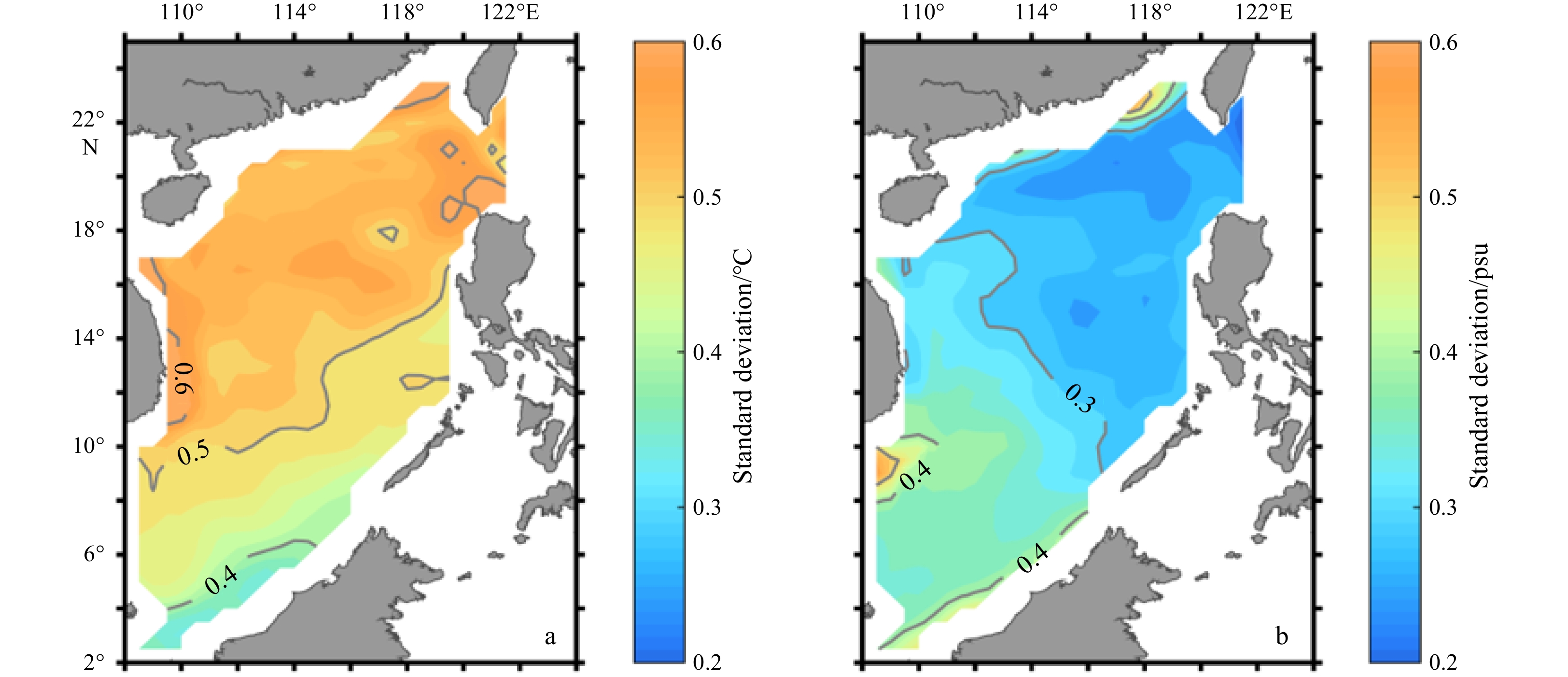
Figure 2 shows the standard deviations of sea surface temperature and salinity anomalies in the SCS in SODA3.4.1. The results show that the strongest interannual variation of sea surface temperature anomalies (SSTA) is in the Luzon Strait and SCSWBC region, with a standard deviation of approximately 0.6°C. The basin scale distribution of SSTA standard deviation generally shows larger values in the northwestern SCS and smaller values in the southeastern SCS. The sea surface salinity anomalies (SSSA) show the strongest interannual variation along the northern slope and in the southeast of Vietnam, with a standard deviation of approximately 0.5. The distribution of SSSA standard deviation is somewhat opposite to that of SSTA, showing larger values in the southwestern SCS and smaller values in the northeastern SCS, except for the northern slope.

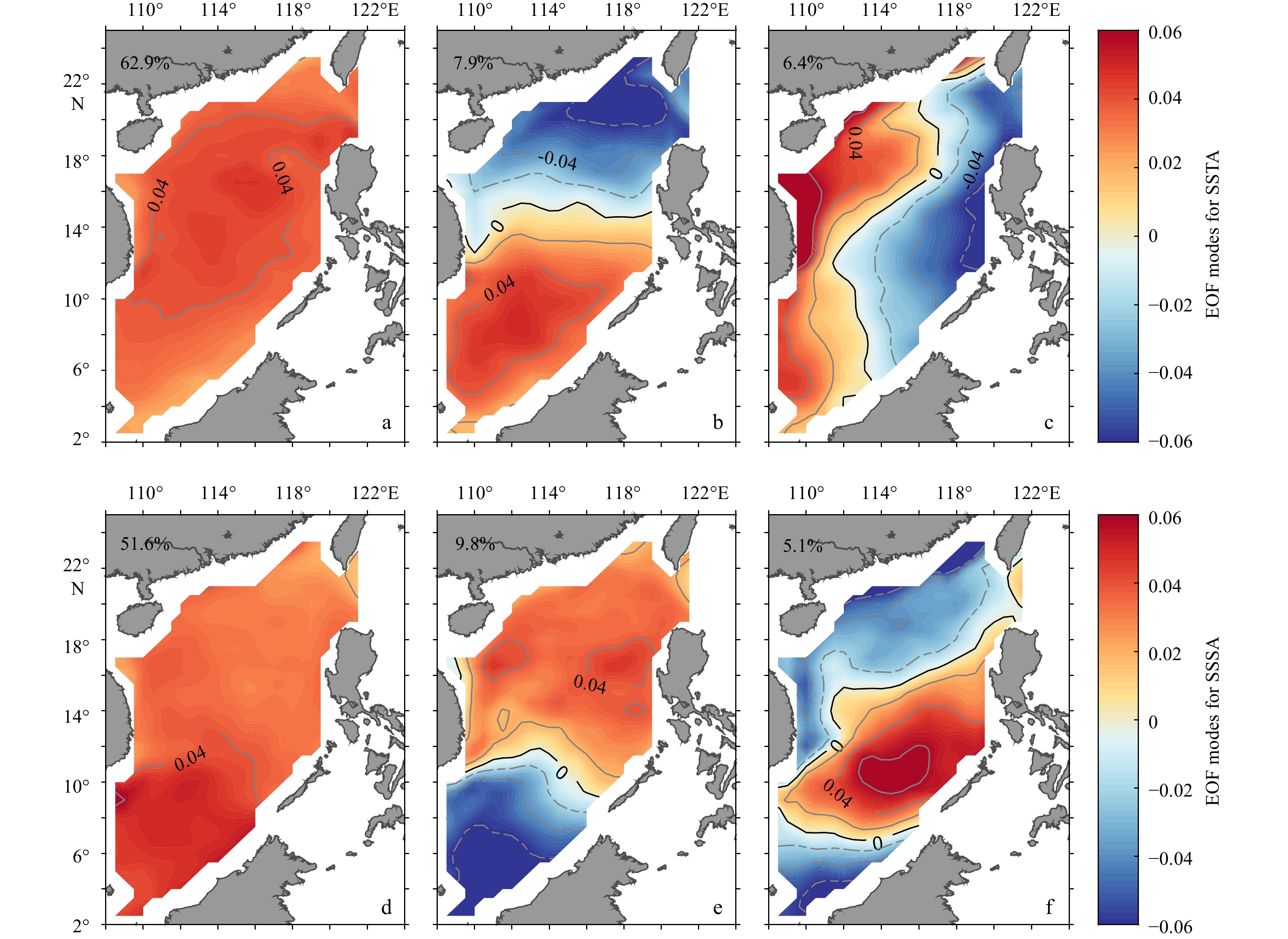
Figure 3 shows the spatial structure of the first three EOF modes of the SSTA and SSSA. The variance contributions of the first three modes are 62.9%, 7.9%, and 6.4% for SSTA and 51.6%, 9.8%, and 5.1% for SSSA. The patterns of the first EOF mode for SSTA and SSSA are reminiscent of their standard deviation, suggesting that most of the interannual variations for SSTA and SSSA can be explained by the first EOF mode (Figs 3a, d). The second EOF mode exhibits a meridional dipole pattern in both SSTA and SSSA (Figs 3b, e). The third EOF mode of SSTA shows positive anomalies in the northwestern SCS and along the SCSWBC region and negative anomalies in the eastern SCS (Fig. 3c). For SSSA, the third EOF mode shows a pattern similar to the first EOF mode of SSTA, but with an opposite sign, i.e., positive anomalies in the southern region of the deep basin (Fig. 3f). Overall, the SODA3.4.1 has well reproduced the dominant EOF modes of SSTA and SSSA in the SCS as compared to previous observations (Fang et al., 2006; Yi et al., 2020).

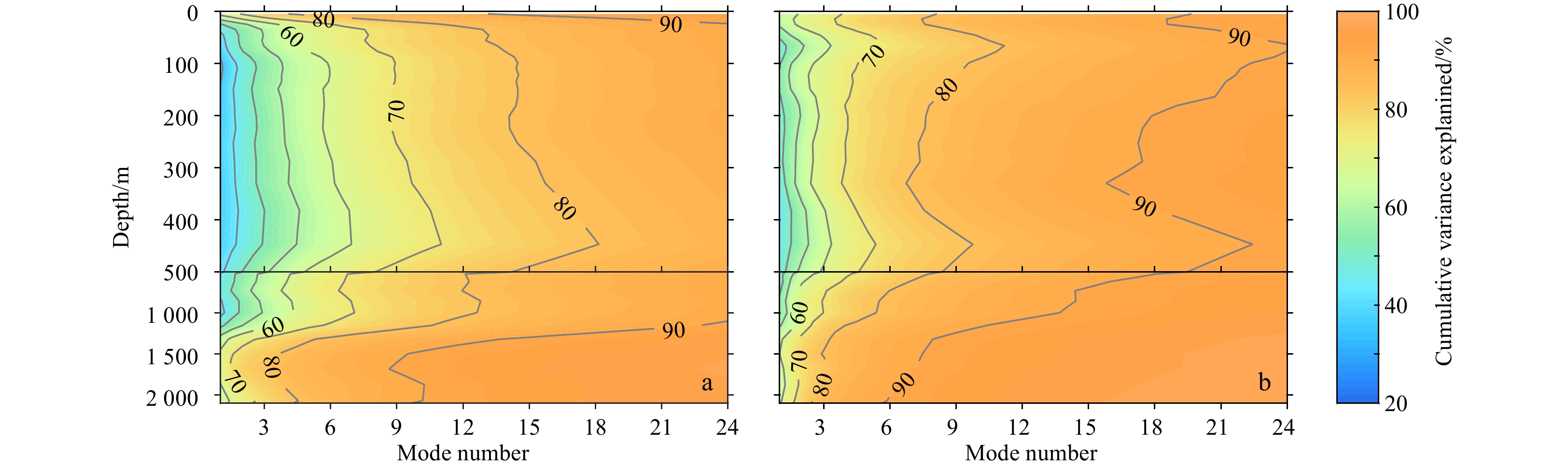
Figure 4 shows the cumulative variation contribution of different numbers of leading EOF modes at different depths for temperature and salinity anomalies. The first 15–18 EOF modes explain more than 80% of the total variance for temperature anomalies in the upper layers. For upper layer salinity, 9–12 EOF modes are needed to explain 80% of the total variance. The EOF analysis for both temperature and salinity requires fewer leading EOF modes to explain 80% of their total variance. The number of EOF modes used in the reconstructed experiment should be less than the number of observation locations. Therefore, the configuration for this EOF approach is 12, 10, 8, 6, and 4 EOF modes at 1–13, 14–25, 26–31, 32, and 33–35 depth layers, respectively.

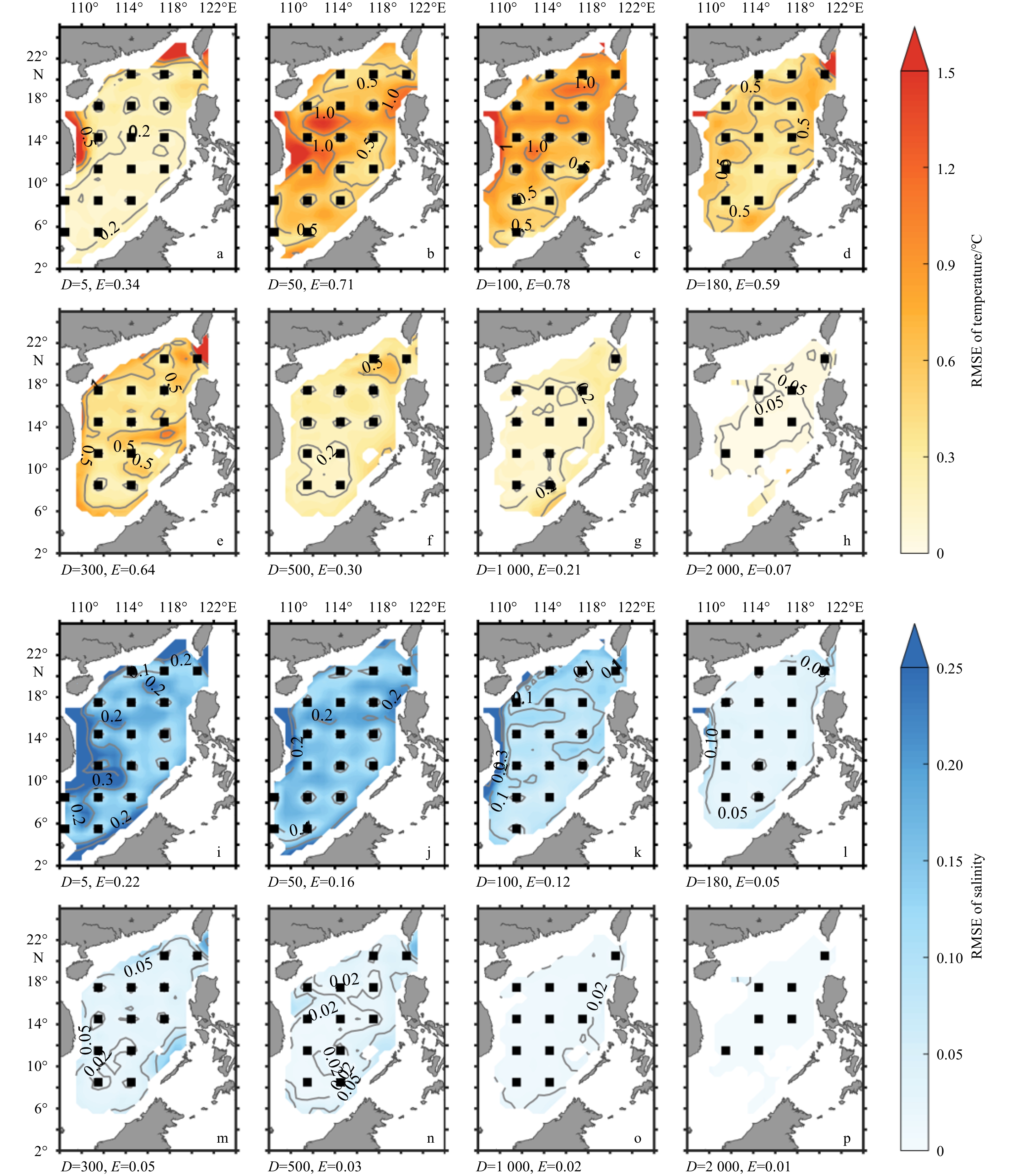
The gridded sea temperature and salinity were reconstructed using values at the grid points of the initial array based on the EOF approach. The RMSE between the reconstructed and raw fields is used to assess the array’s ability to accurately represent the temperature and salinity in the SCS. Figure 5 shows the RMSEs of temperature and salinity at different depths, i.e., 5 m, 50 m, 100 m, 180 m, 300 m, 500 m, 1 000 m, and 2 000 m. The largest RMSEs of SST occur in the northeastern SCS and along the east coast of Vietnam, with values exceeding 1°C. The SST RMSEs in the deep basin are generally around 0.2°C. The RMSEs of temperature in the mixed and thermocline layers are greater than in the surface, intermediate, and deep layers. The largest RMSEs in the mixed and thermocline layers also occur along the east coast of Vietnam, a pattern similar to that of SST, and coincide with the distribution of standard deviation and the first EOF mode of SSTA. The RMSEs of salinity decrease with increasing water depths from area averaged values of approximately 0.22 at the surface, decreasing steadily to 0.01 at 2 000-m depth. The occurrence of the large RMSEs along the east coast of Vietnam and in the northern SCS suggests poor observing ability of the initial array on the SCSWBC.

To obtain the optimal array, the EOF approach was used to conduct a series of OSSEs for different depths. The optimal arrays for temperature and/or salinity at different depths are generally not consistent with one another. The locations of the optimal arrays and corresponding RMSEs distributions are shown in Fig. 6. The observing ability for the SCSWBC is significantly improved, as can be seen by the reduction in temperature and salinity RMSEs of approximately 0.5–1°C at the surface and 0.05–0.2 around 300 m along the east coast of Vietnam. Moreover, the area averaged RMSEs for temperature and salinity of the optimal arrays generally decrease in comparison with those of the initial array at all depths, suggesting overall improvements in the observing ability of the optimal arrays.

It is obviously that the OSSEs would yield different optimal arrays for temperature and/or salinity at different depth layers. If all the locations derived from the OSSEs are considered, the total number of mooring sites is 351, which is not feasible in practice. Therefore, a method is needed to consolidate the dispersed locations into a vertically consistent array. In this study, we use the K-center cluster to consolidate the huge number of potential mooring sites into a limited number of sites. Figure 7 shows the consolidated array with 17 mooring sites. The consolidated array keeps the mooring sites in the northern edge of the initial array but moves the middle and east sites further east. The mooring sites in the central SCS are scattered toward the western and southeastern boundaries of the SCS.

Figure 8 shows the RMSEs of reconstructed temperature and salinity derived from the consolidated array. The largest temperature RMSEs with values exceeding 1°C occur in the northwest of Luzon Strait at the surface, in the central SCS and southwest of the Luzon Strait at 50 m, along the north coast, and in the central and southern regions of the SCS and at 100 m. The largest temperature RMSEs at 180 m and 300 m, with values of approximately 0.5–0.7°C, occur along the pathway of the SCSWBC. The distribution of salinity RMSEs is different from that of temperature. The largest salinity RMSEs generally occur along the pathway of the SCSWBC in the mixed and thermocline layers. In the intermediate and deep layers, the salinity RMSEs show uniform distribution over the deep basin of the SCS. Overall, although the RMSEs of the consolidated array are larger than those of optimal arrays at each depth, the consolidated array still has smaller RMSEs than the initial array at most of the depth layers, except for the temperature at 100 m. These results suggest that the consolidated array is an improvement in the observing ability for three-dimensional temperature and salinity over the initial array.

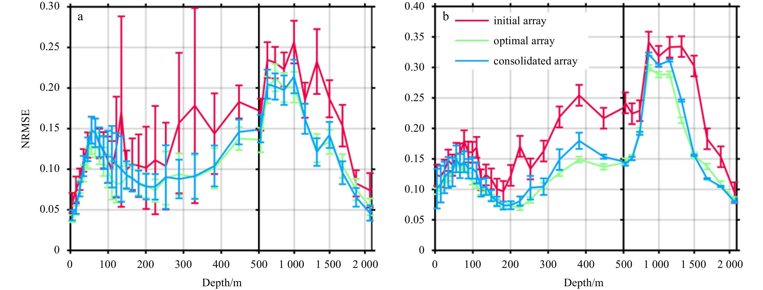
The NRMSE is used to compare the improvement in observing ability between the optimal and consolidated arrays (Fig. 9). The large NRMSEs in temperature for the initial array occur at approximately 300–1 500 m, where values of above 0.15 suggest poor observing ability in intermediate and deep layers. In comparison, the optimal arrays for each depth significantly reduce the NRMSEs below 100 m. The largest reductions occur at 330 m (0.09) and 1 320 m (0.11). The NRMSEs for the consolidated array are basically equivalent to those of the optimal arrays at each depth. The largest difference in the NRMSEs between the consolidated and optimal arrays occurs at 110 m, with values of 0.03. The NRMSEs in salinity decrease with increasing water depth, decreasing rapidly from 0.34 to 0.09 below 800 m and decreasing gently in the upper 800 m. The pattern of changes of salinity NRMSEs at different depths coincides well with that of temperature. The optimal and consolidated arrays also show improvement in the observing ability for salinity, with their normalized RMSE curves nearly coinciding with one another. These results confirm the efficiency of the K-center clustering algorithm in consolidating the optimal arrays.

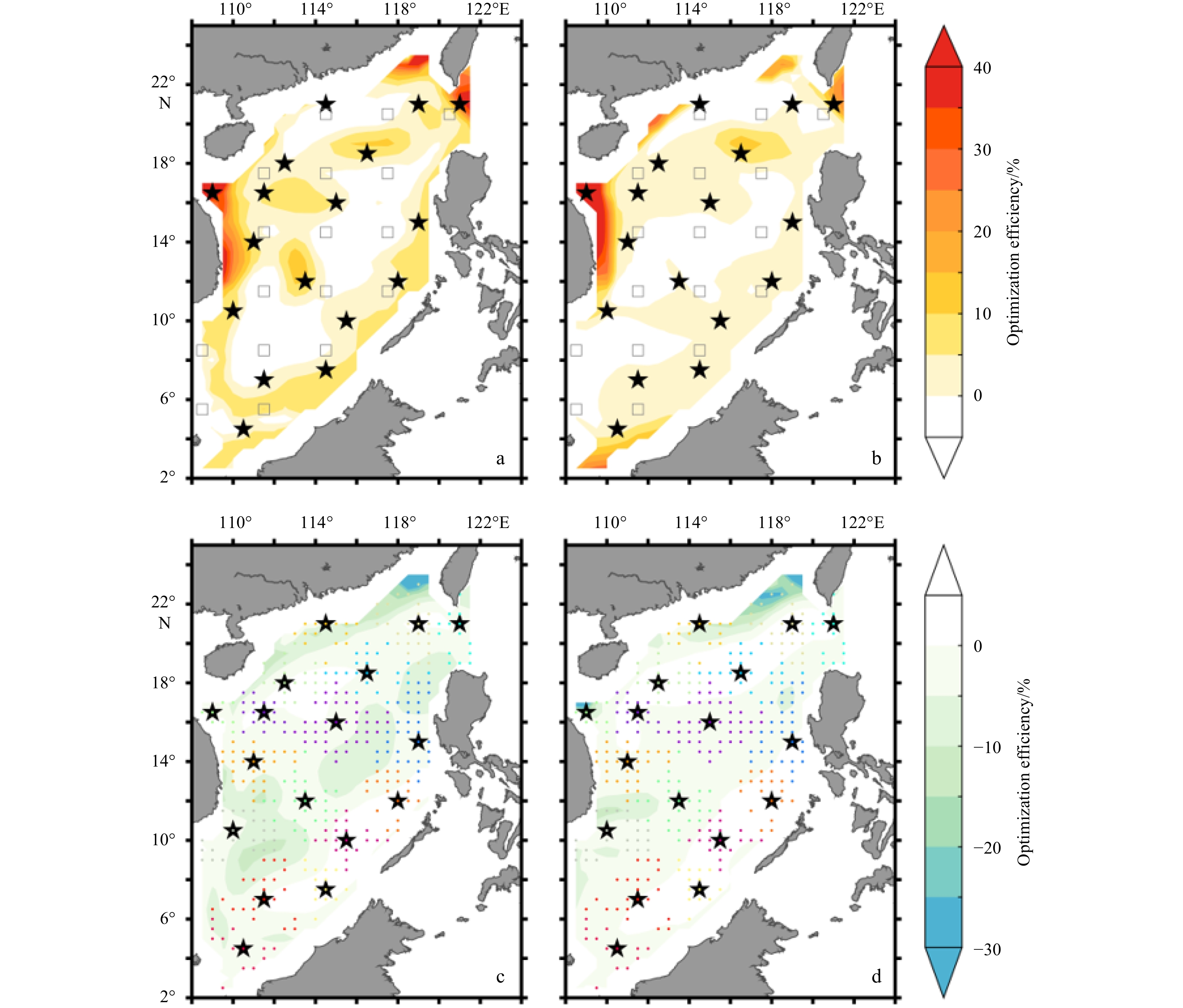
Figure 10 shows the optimization efficiency of the consolidated array in comparison to the initial and optimal arrays. The largest improvement of the observing ability for both temperature and salinity occurs in the Luzon Strait and the SCSWCB region, with optimization efficiency up to approximately 30%–40% (Figs 10a, b). In the deep basin and southern edge of the SCS, the optimization efficiencies are between 5%–10% in temperature, and 0–10% in salinity, respectively. It should be noted that the optimization efficiencies of the consolidated array are lower than the optimal arrays for both temperature and salinity. However, the optimal array for temperature generally does not have good ability in observing salinity, and vice versa. Therefore, in comparison to the overall optimization efficiencies of 23.01% and 26.44% in temperature and salinity for the optimal arrays, the consolidated array, which overall optimization efficiencies are 19.03% and 21.38%, is a considerable scheme for array designment.

By setting different numbers of categories, i.e., the K values in the K-center cluster, we have conducted a series of OSSEs to obtain a set of consolidated arrays with station numbers from 15 to 30. The averaged NRMSEs of temperature and salinity show rapid reductions from 0.13 to 0.10 (temperature) and 0.18 to 0.13 (salinity), while the station number increases from 15 to 20 (Fig. 11a). However, the reductions are only 0.007 and 0.01, when the station number increases from 20 to 30 (Fig. 11a). Therefore, 20 is considered to be the most cost-effective station number for the consolidated array. The selection of 20 for the most cost-effective number of stations is corroborated by the NRMSEs of temperature and salinity at different depths with consolidated arrays consisting of 17, 20, 23, and 26 stations (Figs 11b, c). The NRMSEs drop by 0–0.03 for temperature and 0–0.04 for salinity, when the station number increases from 17 to 20. However, the NRMSEs generally coincide with one another for the consolidated arrays with station numbers of 20, 23, and 26.

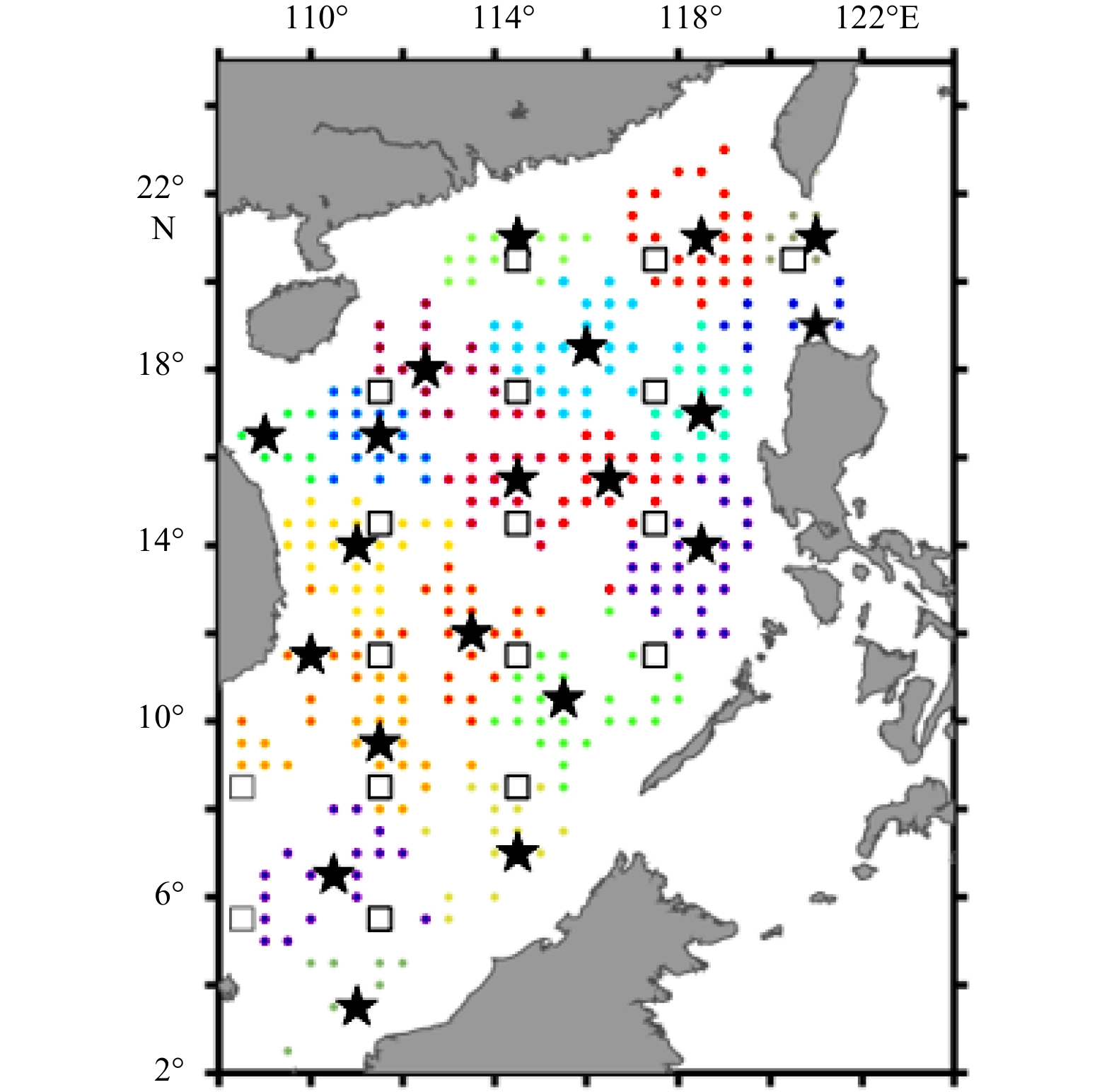
Figure 12 shows a consolidated array consisting of 20 stations, considered to be the most appropriately scaled array for observing three-dimensional temperature and salinity in the SCS. In addition to the fixed scale consolidated array with 17 stations, there is one additional station located in the southern Luzon Strait and two additional stations located in the central SCS basin. The locations along the pathway of the SCSWBC basically do not change, whereas the mooring locations in the southeastern SCS have been slightly modulated.

In this study, we developed a MAOT consisting of the EOF-based approach and the K-center clustering algorithm modules. The MAOT was then used to conduct a series of OSSEs for moored array optimization in the SCS with a focus on three-dimensional temperature and salinity. First, the EOF-based approach was used to obtain a set of optimal arrays independent of one another for temperature and salinity at different depths. Second, the K-center clustering algorithm was used to obtain a consolidated array with determinate mooring locations, based on the optimal arrays set. The optimization efficiencies of the consolidated array are lower than the optimal arrays with only temperature or salinity is considered. However, the optimal array for temperature generally does not have good ability in observing salinity, and vice versa. Therefore, the consolidated array would achieve best performance in synchronously observation for temperature and salinity.
The initial array was assumed to consist of 17 mooring sites, located on a 3°×3° horizontal grid. It should be noted that changes in the initial array configuration (mooring number and locations) do not result in a different consolidated array. Instead, this only leads to different optimization efficiencies. In comparison with the initial array, the overall optimization efficiencies of the consolidated array are 19.03% for temperature and 21.38% for salinity, although there are negative optimization efficiencies in some areas of the SCS. The largest improvement in the observing ability for both temperature and salinity occurs in the Luzon Strait and the SCSWCB region, with optimization efficiencies of up to approximately 30%–40%. In the deep basin and southern edge of the SCS, the optimization efficiencies are between 5%–10% for temperature and 0–10% for salinity. For the optimal arrays, the overall optimization efficiencies are 23.01% for temperature and 26.44% for salinity, which are larger than that of the consolidated array by 3.98% and 5.06%, respectively. The reduction of optimization efficiencies of the consolidated array as compared with the optimal arrays occurs along the north slope of the SCS and in the east of Vietnam.
Optimization efficiency can be further improved by increasing the number of moorings. However, when cost and effectiveness are considered, a cost-effective number of mooring sites for the consolidated array can be determined. Our analyses show that when the mooring number is increased to 20, the optimization efficiencies reach 26.54% for temperature and 27.25% for salinity. However, the optimization efficiencies are not significantly improved when moorings in excess of 20.
An optimal array design should accommodate different purposes, such as studying ocean phenomenon at different spatial and temporal scales. In this study, we focused on basin-scale interannual variations in temperature and salinity in the SCS. The consolidated array we developed may not be adequate to resolve mesoscale processes, such as ocean fronts, mesoscale eddies, and internal waves, as well as sub-mesoscale and small-scale processes. Nevertheless, the MAOT proposed in this study is useful for many applications and could be extended to other regions.
| [1] |
Alvarez A, Mourre B. 2012. Optimum sampling designs for a glider-mooring observing network. Journal of Atmospheric and Oceanic Technology, 29(4): 601–612. doi: 10.1175/JTECH-D-11-00105.1
|
| [2] |
Arnold C P Jr, Dey C H. 1986. Observing-systems simulation experiments: Past, present, and future. Bulletin of the American Meteorological Society, 67(6): 687–695. doi: 10.1175/1520-0477(1986)067<0687:OSSEPP>2.0.CO;2
|
| [3] |
Ballabrera-Poy J, Hackert E, Murtugudde R, et al. 2007. An observing system simulation experiment for an optimal moored instrument array in the tropical Indian Ocean. Journal of Climate, 20(13): 3284–3299. doi: 10.1175/JCLI4149.1
|
| [4] |
Carton J A, Chepurin G A, Chen Ligang. 2018. SODA3: a new ocean climate reanalysis. Journal of Climate, 31(17): 6967–6983. doi: 10.1175/JCLI-D-18-0149.1
|
| [5] |
Fang Guohong, Chen Haiying, Wei Zexun, et al. 2006. Trends and interannual variability of the South China Sea surface winds, surface height, and surface temperature in the recent decade. Journal of Geophysical Research: Oceans, 111(C11): C11S16
|
| [6] |
Feng Rong, Duan Wansuo, Mu Mu. 2017. Estimating observing locations for advancing beyond the winter predictability barrier of Indian Ocean dipole event predictions. Climate Dynamics, 48(3−4): 1173–1185. doi: 10.1007/s00382-016-3134-3
|
| [7] |
Frolov S, Baptista A, Wilkin M. 2008. Optimizing fixed observational assets in a coastal observatory. Continental Shelf Research, 28(19): 2644–2658. doi: 10.1016/j.csr.2008.08.009
|
| [8] |
Fu Weiwei, Høyer J L, She Jun. 2011. Assessment of the three dimensional temperature and salinity observational networks in the Baltic Sea and North Sea. Ocean Science, 7(1): 75–90. doi: 10.5194/os-7-75-2011
|
| [9] |
Fujii Y, Rémy E, Zuo Hao, et al. 2019. Observing system evaluation based on ocean data assimilation and prediction systems: On-going challenges and a future vision for designing and supporting ocean observational networks. Frontiers in Marine Science, 6: 417. doi: 10.3389/fmars.2019.00417
|
| [10] |
Gasparin F, Roemmich D, Gilson J, et al. 2015. Assessment of the upper-ocean observing system in the equatorial Pacific: The role of Argo in resolving intraseasonal to interannual variability. Journal of Atmospheric and Oceanic Technology, 32(9): 1668–1688. doi: 10.1175/JTECH-D-14-00218.1
|
| [11] |
Geng Wu, Cheng Feng, Xie Qiang, et al. 2020. Observation system simulation experiments using an ensemble-based method in the northeastern South China Sea. Journal of Oceanology and Limnology, 38(6): 1729–1745. doi: 10.1007/s00343-019-9119-4
|
| [12] |
Haber J, Zeilfelder F, Davydov O, et al. 2001. Smooth approximation and rendering of large scattered data sets. In: Proceedings of the Conference on Visualization. San Diego, CA: IEEE, 341–348
|
| [13] |
Hackert E C, Miller R N, Busalacchi A J. 1998. An optimized design for a moored instrument array in the tropical Atlantic Ocean. Journal of Geophysical Research: Oceans, 103(C4): 7491–7509. doi: 10.1029/97JC03206
|
| [14] |
Hirschi J, Baehr J, Marotzke J, et al. 2003. A monitoring design for the Atlantic meridional overturning circulation. Geophysical Research Letters, 30(7): 1413
|
| [15] |
Hu Junya, Duan Wansuo. 2016. Relationship between optimal precursory disturbances and optimally growing initial errors associated with ENSO events: Implications to target observations for ENSO prediction. Journal of Geophysical Research: Oceans, 121(5): 2901–2917. doi: 10.1002/2015JC011386
|
| [16] |
Hu Jianyu, Ho C R, Xie Lingling, et al. 2020. Regional Oceanography of the South China Sea. Singapore: World Scientific Publishing Company
|
| [17] |
Huang Xiaodong, Wang Zhaoyun, Zhang Zhiwei, et al. 2018. Role of mesoscale eddies in modulating the semidiurnal internal tide: Observation results in the northern South China Sea. Journal of Physical Oceanography, 48(8): 1749–1770. doi: 10.1175/JPO-D-17-0209.1
|
| [18] |
Huang Xiaodong, Zhang Zhiwei, Zhang Xiaoqiang, et al. 2017. Impacts of a mesoscale eddy pair on internal solitary waves in the northern South China Sea revealed by mooring array observations. Journal of Physical Oceanography, 47(7): 1539–1554. doi: 10.1175/JPO-D-16-0111.1
|
| [19] |
Lermusiaux P F J. 2007. Adaptive modeling, adaptive data assimilation and adaptive sampling. Physica D: Nonlinear Phenomena, 230(1−2): 172–196. doi: 10.1016/j.physd.2007.02.014
|
| [20] |
Li Yineng, Peng Shiqiu, Liu Duanling. 2014. Adaptive observation in the South China Sea using CNOP approach based on a 3-D ocean circulation model and its adjoint model. Journal of Geophysical Research: Oceans, 119(12): 8973–8986. doi: 10.1002/2014JC010220
|
| [21] |
Liang Zhanlin, Xing Tao, Wang Yinxia, et al. 2019. Mixed layer heat variations in the South China Sea observed by Argo float and reanalysis data during 2012–2015. Sustainability, 11(19): 5429. doi: 10.3390/su11195429
|
| [22] |
Liu Danian, Zhu Jiang, Shu Yeqiang, et al. 2018a. Model-based assessment of a northwestern tropical Pacific moored array to monitor intraseasonal variability. Ocean Modelling, 126: 1–12. doi: 10.1016/j.ocemod.2018.04.001
|
| [23] |
Liu Danian, Zhu Jiang, Shu Yeqiang, et al. 2018b. Targeted observation analysis of a northwestern tropical Pacific Ocean mooring array using an ensemble-based method. Ocean Dynamics, 68(9): 1109–1119. doi: 10.1007/s10236-018-1188-y
|
| [24] |
Masutani M, Schlatter T W, Errico R M, et al. 2010. Observing system simulation experiments. In: Lahoz W, Khattatov B, Menard R, eds. Data Assimilation: Making Sense of Observations. Berlin, Heidelberg: Springer, 647–679
|
| [25] |
McIntosh P C. 1987. Systematic design of observational arrays. Journal of Physical Oceanography, 17(7): 885–902. doi: 10.1175/1520-0485(1987)017<0885:SDOOA>2.0.CO;2
|
| [26] |
Mu Mu, Duan Wansuo. 2003. A new approach to studying ENSO predictability: Conditional nonlinear optimal perturbation. Chinese Science Bulletin, 48(10): 1045–1047. doi: 10.1007/BF03184224
|
| [27] |
Oke P R, Sakov P. 2012. Assessing the footprint of a regional ocean observing system. Journal of Marine Systems, 105–108: 30–51
|
| [28] |
Oke P R, Schiller A. 2007. A model-based assessment and design of a tropical Indian Ocean mooring array. Journal of Climate, 20(13): 3269–3283. doi: 10.1175/JCLI4170.1
|
| [29] |
Palmer T N, Gelaro R, Barkmeijer J, et al. 1998. Singular vectors, metrics, and adaptive observations. Journal of the Atmospheric Sciences, 55(4): 633–653. doi: 10.1175/1520-0469(1998)055<0633:SVMAAO>2.0.CO;2
|
| [30] |
Park H S, Jun C H. 2009. A simple and fast algorithm for K-medoids clustering. Expert Systems with Applications, 36(2): 3336–3341. doi: 10.1016/j.eswa.2008.01.039
|
| [31] |
Peng Hanbang, Pan Aijun, Zheng Quanan et al. 2018. Analysis of monthly variability of thermocline in the South China Sea. Journal of Oceanology and Limnology, 36(2): 205–215. doi: 10.1007/s00343-017-6151-0
|
| [32] |
Sakov P, Oke P R. 2008. Objective array design: Application to the tropical Indian Ocean. Journal of Atmospheric and Oceanic Technology, 25(5): 794–807. doi: 10.1175/2007JTECHO553.1
|
| [33] |
Sun Zhongbin, Zhang Zhiwei, Qiu Bo, et al. 2020. Three-dimensional structure and interannual variability of the Kuroshio loop current in the northeastern South China Sea. Journal of Physical Oceanography, 50(9): 2437–2455. doi: 10.1175/JPO-D-20-0058.1
|
| [34] |
Thomson R E, Emery W J. 2014. Data Analysis Methods in Physical Oceanography. 3rd ed. New York: Elsevier, 335–356
|
| [35] |
Vecchi G A, Harrison M J. 2007. An observing system simulation experiment for the Indian Ocean. Journal of Climate, 20(13): 3300–3319. doi: 10.1175/JCLI4147.1
|
| [36] |
Wang Zhaoyun, Huang Xiaodong, Yang Yunchao, et al. 2020. Impacts of subtidal motions and the earth rotation on modal characteristics of the semidiurnal internal tide. Journal of Oceanography, 76(1): 15–27. doi: 10.1007/s10872-019-00524-7
|
| [37] |
Wei Zexun, Li Shujiang, Susanto R D, et al. 2019. An overview of 10-year observation of the South China Sea branch of the Pacific to Indian Ocean throughflow at the Karimata Strait. Acta Oceanologica Sinica, 38(4): 1–11. doi: 10.1007/s13131-019-1410-x
|
| [38] |
Xiao Fuan, Wang Dongxiao, Zeng Lili, et al. 2019. Contrasting changes in the sea surface temperature and upper ocean heat content in the South China Sea during recent decades. Climate Dynamics, 53(3−4): 1597–1612. doi: 10.1007/s00382-019-04697-1
|
| [39] |
Xue Pengfei, Chen Changsheng, Beardsley R C, et al. 2011. Observing system simulation experiments with ensemble Kalman filters in Nantucket Sound, Massachusetts. Journal of Geophysical Research: Oceans, 116(C1): C01011
|
| [40] |
Yang Qingxuan, Tian Jiwei, Zhao Wei. 2007. Observation of Luzon Strait transport in summer 2007. Deep-Sea Research Part I: Oceanographic Research Papers, 57(5): 670–676
|
| [41] |
Yang Lei, Wang Dongxiao, Huang Jian, et al. 2015. Toward a mesoscale hydrological and marine meteorological observation network in the South China Sea. Bulletin of the American Meteorological Society, 96(7): 1117–1135. doi: 10.1175/BAMS-D-14-00159.1
|
| [42] |
Yi Dalingli, Melnichenko O, Hacker P, et al. 2020. Remote sensing of sea surface salinity variability in the South China Sea. Journal of Geophysical Research: Oceans, 125(12): e2020JC016827
|
| [43] |
Yildirim B, Chryssostomidis C, Karniadakis G E. 2009. Efficient sensor placement for ocean measurements using low-dimensional concepts. Ocean Modelling, 27(3–4): 160–173. doi: 10.1016/j.ocemod.2009.01.001
|
| [44] |
Zeng Lili, Wang Qiang, Xie Qiang, et al. 2015. Hydrographic field investigations in the northern South China Sea by open cruises during 2004–2013. Science Bulletin, 60(6): 607–615. doi: 10.1007/s11434-015-0733-z
|
| [45] |
Zhang Yanwu, Bellingham J G. 2008. An efficient method of selecting ocean observing locations for capturing the leading modes and reconstructing the full field. Journal of Geophysical Research: Oceans, 113(C4): C04005
|
| [46] |
Zhang Kun, Mu Mu, Wang Qiang. 2017. Identifying the sensitive area in adaptive observation for predicting the upstream Kuroshio transport variation in a 3-D ocean model. Science China Earth Sciences, 60(5): 866–875. doi: 10.1007/s11430-016-9020-8
|
| [47] |
Zhang Kun, Mu Mu, Wang Qiang, et al. 2019. CNOP-based adaptive observation network designed for improving upstream Kuroshio transport prediction. Journal of Geophysical Research: Oceans, 124(6): 4350–4364. doi: 10.1029/2018JC014490
|
| [48] |
Zhang Kun, Mu Mu, Wang Qiang. 2020. Increasingly important role of numerical modeling in oceanic observation design strategy: A review. Science China Earth Sciences, 63(11): 1678–1690. doi: 10.1007/s11430-020-9674-6
|
| [49] |
Zhang Zhiwei, Zhao Wei, Tian Jiwei, et al. 2015. Spatial structure and temporal variability of the zonal flow in the Luzon Strait. Journal of Geophysical Research: Oceans, 120(2): 759–776. doi: 10.1002/2014JC010308
|
| [50] |
Zhao Wei, Zhou Chun, Tian Jiwei, et al. 2014. Deep water circulation in the Luzon Strait. Journal of Geophysical Research: Oceans, 119(2): 790–804. doi: 10.1002/2013JC009587
|
| [51] |
Zhou Chun, Zhao Wei, Tian Jiwei, et al. 2017. Deep western boundary current in the South China Sea. Scientific Reports, 7: 9303. doi: 10.1038/s41598-017-09436-2
|
| [52] |
Zhu Yaohua, Fang Guohong, Wei Zexun, et al. 2016. Seasonal variability of the meridional overturning circulation in the South China Sea and its connection with inter-ocean transport based on SODA2.2.4. Journal of Geophysical Research: Oceans, 121(5): 3090–3105. doi: 10.1002/2015JC011443
|

Figures(12)

Supported by:
Beijing Renhe Information Technology Co. Ltd

Mengxue Qu, Zexun Wei, Yanfeng Wang, Yonggang Wang, Tengfei Xu. Objective array design for three-dimensional temperature and salinity observation: Application to the South China Sea[J]. Acta Oceanologica Sinica, 2022, 41(7): 65-77. doi: 10.1007/s13131-021-1975-z

 DownLoad:


 DownLoad: