Vertical velocity and transport in the South China Sea

1. Introduction

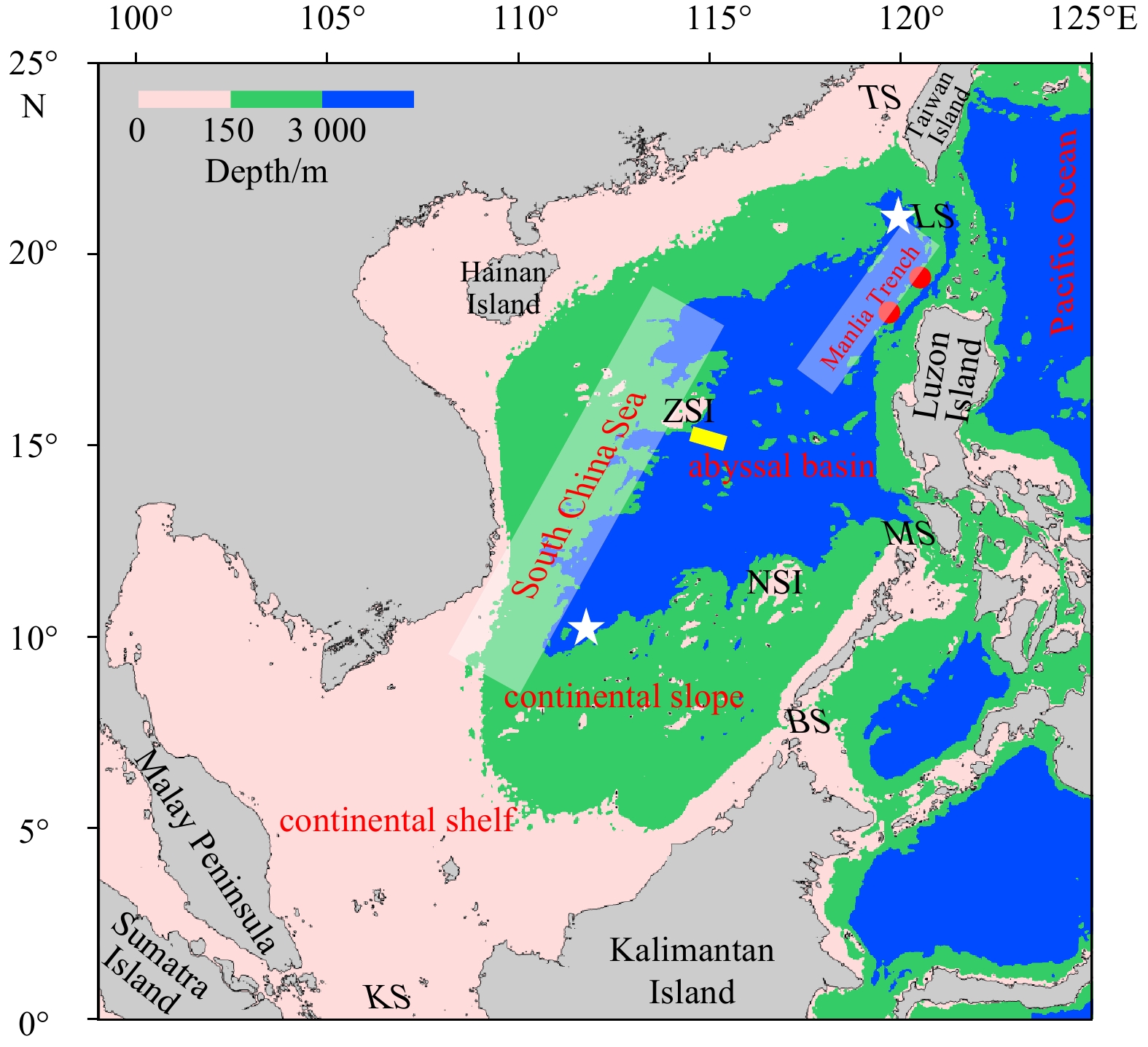
The South China Sea (SCS) covers an area of 3.5×10⁶ km², including 1.68×10⁶ km² on continental shelves, 1.26×10⁶ km² on slopes and 0.55×10⁶ km² in the abyssal basin below 3 000 m (Fig. 1). In view of the 200 m isobath, it is a semienclosed oceanic basin (Wang, 1986). The SCS connects to the western Pacific through its sole deepwater renewal channel, the Luzon Strait, with the deepest sill at about 2 400 m. Below the depth of 1 500 m, the density on both sides of the Luzon Strait bifurcates, and water is denser on the Pacific side than that on the SCS side. As a result, there exists a persistent pressure gradient across the Luzon Strait, driving a so-called Luzon Strait deepwater overflow from the Pacific into the SCS (Nitani, 1972; Qu et al., 2006; Li and Qu, 2006; Zhao et al., 2014; Zhang et al., 2015). The bifurcation depth of water density, about 1 500 m, is thus considered as the upper interface of the Luzon Strait overflow. After the dense Pacific water sinks into the SCS through the gaps in the Heng-Chun Ridge, the abyssal water in the SCS is renewed and must upwell somewhere. Then, scientific questions arise. At what depth and from where the abyssal water upwells? What is the causal mechanism?

Figure  1.  Topography of the South China Sea. The abbreviations LS, TS, KS, MS, BS denote the Luzon Strait, Taiwan Strait, Karimata Strait, Mindoro Strait, Balabac Strait, respectively; and ZSI and NSI denote the Zhongsha Islands and Nansha Islands, respectively. Yellow line indicates the mooring section deployed off the Zhongsha Islands in Zhou et al. (2017). White stars represent the northern and southern ends of the abyssal basin below 3 000 m, where the abyssal water upwells. Red dots stand for gaps in the Heng-Chun Ridge, through which the Luzon Strait overflow sinks into the Manila Trench.

DownLoad: Full-Size Img PowerPoint

Vertical velocity in the SCS has been studied as an important index of regional upwelling and downwelling. Among previous studies, Chai et al. (2001) analyzed formation of upwelling in the nearshore areas and Gan et al. (2013) focused on dynamics of the intensified downwelling over a widened northern SCS continental shelf. Xie et al. (2012), Jing et al. (2015) and Xie et al. (2017) investigated the vertical circulation and its dynamics on the continental shelf east of Hainan Island. Qu (2000) and Qu et al. (2007) discussed offshore upwelling in the upper layer using historical temperature profiles, while Chao et al. (1996), Shu et al. (2014), and Cai and Gan (2020) analyzed vertical velocity in the deep layer using numerical models. Until now, an overall look of the vertical velocity and associated transport in the SCS basin scale is not in focus yet, however, it is an important part of vertical circulation and also links the layered horizontal circulation. Our objective of this study is to reveal the spatial pattern of vertical velocity and structure of vertical transport. Further, we devote to the mechanism how the vertical velocity arises from the abyssal basin, and mechanism how the vertical transport is forced. Finally, we analyze the role of vertical velocity and vertical transport, and then diagram the three-dimensional circulation in the SCS.

The rest of the paper is organized as follows. In Section 2, we describe the method and validate the data used in this study. Section 3 is devoted to the vertical velocity and mechanism of the vertical transport in the thermocline. Section 4 focuses on the vertical velocity and transport in the deepwater cell. A possible mechanism of upward velocity in the abyssal basin is proposed in Section 5, followed by a summary and conclusions in Section 6.

2. Data and methods

2.1 Data

The 22-year (1994–2015) product of Hybrid Coordinate Ocean Model+Navy Coupled Ocean Data Assimilation (HYCOM+NCODA) (1/12)° reanalysis run by the Naval Research Laboratory of U.S. Navy is analyzed in this study (available at http://hycom.org/dataserver/glb-reanalysis). This HYCOM Global Ocean Forecasting System (GOFS) version 3.1 reanalysis is of significant improvements over its previous version, GOFS3.0. In detail, it has 17 terms in the equation of state, instead of only 7 terms in the GOFS3.0 version; it has 41 vertical layers, instead of only 32 layers in the GOFS3.0; it calculates wind stress using sea surface temperature (SST) and taking into account surface currents, instead of reading in the off-line wind stress in the previous version. The HYCOM GOFS3.1 also has advantages in calculating ocean turbidity from monthly chlorophyll climatology, instead of using photosynthetically available radiation in the GOFS3.0; it uses weaker sea surface salinity (SSS) relaxation, instead of strong relaxation in the GOFS3.0 version.

2.2 Validation of HYCOM GOFS3.1 reanalysis

As vertical velocity in the thermocline and deep cells will be discussed in the following sections, here we validate the HYCOM GOFS3.1 reanalysis with observations in both shallow water and deep layer, respectively. The most remarkable feature in the deep SCS circulation is the deep western boundary current (DWBC). Among all the available in situ current observations in the DWBC, the velocity profiles east of Zhongsha Islands with 6 moorings during August 2012 to January 2014 observed by Zhou et al. (2017) are probably the longest mooring data. The time-mean alongshore velocity from observations manifests a southwestward DWBC core leaning on the continental slope margin with a maximum magnitude of 2 cm/s and standard deviation (STD) up to 5 cm/s above the bottom (Fig. 2a). These main features are favorably simulated by the HYCOM GOFS3.1 reanalysis albeit the DWBC core is overestimated. The standard deviation in the DWBC core from the HYCOM reaches 4.5 cm/s, corresponding well to the observations (Fig. 2b). The discrepancies of core depth, strength and thickness of the DWBC between the HYCOM GOFS3.1 reanalysis and the mooring observations are probably due to the coarse vertical resolution in the model (with a layer thickness of 500 m near the bottom) and topographic difference between reality and numerical model. The monthly mean alongshore velocity in the DWBC core reaches its maximum in April, 7.2 cm/s from the observations (Fig. 2c) and 6.8 cm/s from the HYCOM reanalysis (Fig. 2d). The monthly climatology of the DWBC from both observations and HYCOM reanalysis shows a robust southwestward core from April to September and weak DWBC from October to March. Considering the velocity in the deep layer is much more difficulty to simulate than that near the sea surface and the flow is not constrained by the data assimilation below 2 000 m, the HYCOM GOFS3.1 reanalysis is deemed to reproduce the bottom-intensified DWBC and show a decent agreement with the long-term observations in the location, strength, stand deviation, and monthly climatology of the DWBC core.

Figure  2.  Time-mean alongshore velocity in the deep western boundary current (DWBC) east of Zhongsha Islands from mooring observations (a), after Zhou et al. (2017), and HYCOM GOFS3.1 reanalysis (b). In a and b, color shading indicates the time-mean velocity, positive southwestward. Gray shading represents the topography. Black lines stand for the standard deviation of the alongshore velocity. Monthly mean alongshore velocity in the DWBC core east of Zhongsha Islands during August 2012 to September 2013 from mooring observations (c), after Zhou et al. (2017), and HYCOM GOFS3.1 reanalysis (d). In c and d, standard deviations are indicated by red bars.

DownLoad: Full-Size Img PowerPoint

Time-series of volume transport is often used to examine model results. Among all the main passages connecting the SCS and adjacent oceans, the Karimata Strait is of the longest record of volume transport estimated with direct measurements of current and satellite observations from 2008 to 2016 (Xu et al., 2021). For a better comparison, this observational transport series is extended based on sea surface height and local wind from satellite to cover the HYCOM GOFS3.1 reanalysis. The 22-year monthly mean volume transport through the Karimata Strait from the HYCOM is depicted in Fig. 3a (black line). It agrees well with observational monthly mean transport (red line). The time-mean transport is 0.82×10⁶ m³/s southward from observations and 0.62×10⁶ m³/s southward from the HYCOM GOFS3.1 reanalysis, which is well within the standard error of estimate from the observations (0.48×10⁶ m³/s). In the meantime, the HYCOM GOFS3.1 reanalysis captures the temporal variability of the transport fairly well. The correlation coefficient between the two transport time series is 0.98 and above the 95% confidence level.

Figure  3.  Comparison of monthly mean transport from the HYCOM GOFS3.1 reanalysis (black) with that from observations (red) in the Karimata Strait (a), and with along channel velocity (red) observed in the Luzon Trough (b). In a, positive transport is flow into the SCS and negative transport is flow into the Java Sea through the Karimata Strait. In b, negative velocity/transport indicates westward flow; bars indicate the standard deviations.

DownLoad: Full-Size Img PowerPoint

The temporal variability of the Luzon Strait overflow is also examined. The longest record of the Luzon Strait overflow is the 3.5-year continuously mooring-observed along channel velocity (Zhou et al., 2014). The HYCOM GOFS3.1 reanalysis captures an in phase annual cycle with the mooring observations (Fig. 3b). The correlation coefficient between them is 0.60 and above the 95% confidence level. As there is no data assimilation in the abyssal channel, the deepwater flow is always much harder to simulate than the shallow flow does. In addition, deepwater flow is highly topography steered and topography discrepancy does exist between the reality and model. In this sense, we deem the HYCOM GOFS3.1 reanalysis is consistent with observations in both shallow water and deep layer, and thus believe the decent validation of the HYCOM reanalysis may provide a good opportunity in its performance in simulating vertical velocity and transport in the SCS.

2.3 Methods

Over step-like bottom topography as is in the numerical model, vertical velocity is zero at the locally flat ocean floor. Hence, the vertical velocity is calculated by depth-integrating the divergence of horizontal velocity,

where H is the bottom depth, $\vec{V}_{{\rm{h}}}$ is the horizontal velocity vector and z is the depth. To remove grid-scale noise, horizontal smoothing operations are normally used. For example, Chao et al. (1996) smoothed the vertical velocity four times by a Laplacian filter. In the present study, we use a nine-point smoothing algorithm. The horizontal smoothing operation does not change the integration of vertical transport. The domain-integrated vertical transport is derived from

3. Vertical velocity and transport in the thermocline

3.1 Vertical transport

Influenced by wind stress at the sea surface and replenished by overflow in the deep layer, marginal seas are likely of a vertical transport separated into upper and deep layers. For example, in the Banda Sea, a layer of minimum upward transport near 600 m separates upwelling within the thermocline from a deepwater upwelling pattern driven by the deep overflow in the Lifamatola Passage (Gordon et al., 2010). Based on the HYCOM GOFS3.1 reanalysis, we found that the time-mean domain-integrated vertical transport in the SCS can also be divided into two segments, in detail, a thermocline cell and a deepwater cell separated by a minimum vertical transport level at about 250 m depth. In the abyssal basin, the domain-integrated vertical transport $ {V}_{\left(z\right)} $ begins to increase upward from zero at 4 000 m to a maximum of 1.5×10⁶ m³/s at about 1 500 m. Then, it decreases upward to a minimum layer of vertical transport at about 250 m. In the thermocline cell, $ {V}_{\left(z\right)} $ increases upward from 250 m to the other maximum of 1.6×10⁶ m³/s at about 50 m before it decreases upward to zero at the sea surface (Fig. 4a). This two-segmented vertical transport is also derived from other independent reanalysis products. For example, the HYCOM GOFS3.0 reanalysis depicts two vertical cells of transport with a minimum vertical transport at about 600 m (Fig. 4c) while the SODA3.4.2 reanalysis shows a separating depth at the depth of 500 m (figure not shown). The depth of the maximum upward transport in the thermocline occurs at 50 m from the HYCOM GOFS3.1 and SODA3.4.2 reanalysis, and about 60 m from the HYCOM GOFS3.0 reanalysis. Although the minimum layer of the vertical transport may vary with models, the two-segmented feature is robust. In other word, a minimum layer of vertical transport occurs near the bottom of the thermocline, and maximum transport occurs near the depth of Taiwan Strait sill and upper interface of the Luzon Strait overflow, respectively. Hereinafter, the distribution of vertical velocity and structure of vertical transport are derived from the HYCOM GOFS3.1 reanalysis.

Figure  4.  Domain-integrated vertical transport (a) and domain-averaged vertical velocity (b) from the HYCOM GOFS3.1 reanalysis; domain-integrated vertical transport from the HYCOM GOFS3.0 reanalysis (c); separately integrated upward transport and downward transport from the HYCOM GOFS3.1 reanalysis (d).

DownLoad: Full-Size Img PowerPoint

In the thermocline, the vertical transport varies with season due to the influence of monsoon. It manifests an upward section and a downward section in winter. Namely, the upward transport exists in the upper 150 m with its maximum occurring at 40 m, while the downward transport occurs between 150 m and 600 m with the downward maximum of −0.4×10⁶ m³/s at 250 m. In summer, the vertical transport maintains upward with its maximum of 2.5×10⁶ m³/s at 60 m and minimum of 2.2×10⁶ m³/s at about 250 m.

The vertical transport in the SCS is closely related to the flows between the SCS and adjacent seas. According to the numerical experiments carried out by Metzger and Hurlburt (1996) with a global model domain, the cyclonic circulation around the Philippines, which involves a westward flow in the Luzon Strait, a southward flow in the Sulu Archipelago, and an eastward flow in the Sulawesi Sea, is primarily a function of large-scale wind forcing over the Pacific Ocean and model geometry. This opinion was soon verified by Qu (2000), who applied Godfrey’s (1989) “island rule” to the Philippines and interpreted Luzon Strait transport as a result of counterbalance between the basin-scale wind forcing over the Pacific Ocean and the friction created in the shallow passages that connect the SCS with its surrounding oceans. Further, Wang et al. (2006) used “island rule” to examine interannual variability of Luzon Strait transport and found that wind stress in the western and central equatorial Pacific Ocean is the key factor regulating the interannual variability of the Luzon Strait transport. Therefore, “island rule” is the primary forcing responsible for the Luzon Strait inflow and shallow-passage outflows. In addition, the local winds also play a nonnegligible role in volume fluxes through the shallow passages, by means of Ekman drift or Ekman transport. The total Ekman drift through all the straits is out from the SCS, in detail, 0.3×10⁶ m³/s, 0.73×10⁶ m³/s and 0.24×10⁶ m³/s in the time-mean, winter, and summer, respectively. Combined with both effects of remote wind forcing over the Pacific Ocean and local wind stress in the shallow passages, the total flow in the surface layer is out from the SCS (Table 1). As shown in Table 1, the net outflow in the upper 50 m is 1.27×10⁶ m³/s, 0.79×10⁶ m³/s, and 2.13×10⁶ m³/s in the time-mean, winter, and summer, respectively. In order to compensate the excessive outflow in the shallow depths, the subsurface water in the SCS has to be “pulled” upwards to maintain conservation of mass. Thus, the upward vertical transport in the thermocline is largely driven by the combination of the remote wind forcing over the Pacific Ocean and local wind stress in the straits, by means of “island rule” and the Ekman drift, respectively. The maximum vertical transport occurs approximately at 50 m, which is about the sill depth of the Karimata Strait and Taiwan Strait. Above this depth, the total outflow is contributed from the Mindoro Strait, Karimata Strait and Taiwan Strait, whereas below this depth, only the Mindoro Strait contributes and total outflow reduces.

Table  1.  Outflows in the upper 50 m (positive outward from the SCS, unit: 10⁶ m³/s)

	Luzon St.	Taiwan St.	Mindoro St.	Balabac St.	Karimata St.	Net outflow
Mean	−0.39 (−0.09)	1.25 (0.11)	0.09 (0.24)	−0.27 (0.04)	0.59	1.27 (0.3)
Winter	−1.81 (−0.54)	0.17 (0.47)	0.51 (0.96)	−0.42 (−0.16)	2.34	0.79 (0.73)
Summer	1.17 (0.20)	2.60 (−0.04)	−0.23 (−0.15)	−0.24 (0.23)	−1.17	2.13 (0.24)
Note: The numbers in brackets indicate contribution from the Ekman drift.

 | Show Table

DownLoad: CSV

3.2 Horizontal distribution of vertical velocity

In the SCS, the wind regime is controlled by the East Asian monsoon with northeasterly wind in winter and southwesterly wind in summer. As a response to the local wind, the Ekman transport induced vertical velocity mainly exists on the continental shelves and is seasonal reversal. Downward velocity occurs in the western boundary of the SCS in winter and eastern boundary in summer and fall. Oppositely, upward velocity appears in the nearshore area west of Luzon Island in winter, and on the continental shelves off Vietnam and the southern China in spring and summer. As vertical velocity on continental shelves has been profoundly studied (Chai et al., 2001; Gan et al., 2013; Jing et al., 2015; Xie et al., 2012, 2017), hereinafter, the analysis is more focused on the vertical velocity in the deep SCS basin.

As the time-mean vertical transport reaches a maximum at 50 m and minimum at 250 m, the horizontal distribution of the time-mean vertical velocity at 50 m and 250 m is discussed in the following, representing vertical velocity at typical depths in the thermocline cell.

The time-mean wind stress curl over the SCS has a dipole pattern: anticyclonic curl in the north and cyclonic curl in the south, with the zero-wind stress curl line located from 15°N, 110°E to 20°N, 120°E (Qu, 2000). Accordingly, downward velocity at 50 m prevails on the north side of the zero-wind stress curl line (Fig. 5a), roughly along the 500 m isobath off the southern China. Upward velocities are found on both shoreward and seaward sides of this downward velocity band, roughly along the 100 m and 2 000 m isobaths, respectively, showing an alternating upward-downward band structure in the cross-shelf direction. This alternating upward-downward structure from the coast to deep waters was first proposed by Xie et al. (2017) and attributed to the alternating distribution of kinematic deformation, ageostrophic advection, and vertical mixing rate in the cross-shelf direction. Although the mechanism is derived from a diagnosis of three-dimensional vertical circulation in the upwelling and frontal zones on the continental shelf off China, the alternating band structure of the dynamic terms in the cross-shelf direction is apparently applicable to continental slopes and deep basin in the SCS.

Figure  5.  Time-mean vertical velocity (w) at 50 m (a), and 250 m (b), and time-mean horizontal velocity field at 50 m (c), and 250 m (d). The isobaths at 100 m, 500 m, 1 000 m, 2 000 m, and 3 000 m are indicated.

DownLoad: Full-Size Img PowerPoint

Energetic upward velocity prevails to the west of Luzon Island (called the west Luzon eddy in Qu (2000) and Qu et al. (2007)) and is attributed to the strong positive wind stress curl there. Corresponding to the west Luzon eddy, a large cyclonic gyre is clearly seen in the horizontal current field (Fig. 5c). Upward velocity is remarkable east of Vietnam and north of Kalimantan due to the positive wind stress curl there. Generally, vertical velocity in the thermocline cell is stronger in the northern SCS than that in the southern SCS owing to the relatively strong wind stress curl and energetic entrainments and detrainments induced by the Kuroshio intrusion in the northern SCS.

At 250 m depth, although the domain-integrated vertical transport weakens, the vertical velocity is still energetic, reflecting strong entrainments and detrainments at this level. As we have estimated, both upward transport and downward transport reach up to 13×10⁶ m³/s. This indicates that the entrainments and detrainments are greater than the net vertical transport at least by one order (Fig. 4d). Terrain dependent vertical velocity occurs along the continental shelf and slope due to the slope current interacting with the meandering bottom topography (Figs 5a, b). When the bottom currents encounter a convex/concave slope, the upslope/downslope velocity generates (Gan and Allen, 2002; Song and Chao, 2004; Cai and Gan, 2020). The upwelling zone occurs near 13°N east of Vietnam and corresponds to an eastward offshore jet which can be seen from the horizontal velocity field (Fig. 5d). Upwelling there is a compensation to the eastward volume transport. The aforementioned alternating upward-downward band structure in the cross-shelf direction is clearly shown on the horizontal plane (Fig. 5b) and vertical transects (Fig. 6).

Figure  6.  Alternating bands of the upward-downward velocity (w) seen from vertical sections in the thermocline cell.

DownLoad: Full-Size Img PowerPoint

Monsoon induced vertical velocity experiences a seasonal reversal, particularly in the nearshore areas. In winter, the zero-wind stress curl line is roughly located from 5°N, 105°E to 20°N, 120°E with positive values in the south and negative ones in the north. As a result, at 50 m depth, strong downward velocity band appears on the north side of the 500 m isobath off the southern China (Fig. 7a). Upwelling west of Luzon Island corresponds to the local cyclonic wind stress curl, while downward velocity east of Vietnam is attributed to the resultant of the downward Ekman pumping and onshore Ekman transport. At 250 m, the Ekman transport induced downward velocity nearly vanishes along the northern slope and western boundary (Fig. 7b). Vertical velocity can be identified over a dramatically changing topography, for instance, along Vietnam coast. When the WBC flows southward to 13°N along Vietnam coast, the water depth becomes deeper. According to conservation of potential vorticity, i.e., $ （f+\zeta ）/h= $constant, a positive relative vorticity forms accompanying with upwelling. When the WBC flows further southward to 10°N, the water depth becomes shallower. Accordingly, a negative relative vorticity generates accompanying with downwelling below the 200 m depth (Fig. 7b).

Figure  7.  Vertical velocity (w) at 50 m (a), and 250 m (b) in winter, and at 50 m (c), and 250 m (d) in summer. The isobaths at 100 m, 500 m, 1 000 m, 2 000 m, and 3 000 m are indicated.

DownLoad: Full-Size Img PowerPoint

In summer, as a response to the southwesterly monsoon, the Ekman transport induced nearshore upward velocities intensify along the continental shelves off Vietnam and the southern China (Fig. 7c). Under the effect of local wind stress and shelf topography, a northward WBC and a southward WBC converge and form a strong offshore current near 13°N east of Vietnam. Upwelling in the vicinity has been reported in literature (Shaw and Chao, 1994; Chu et al., 1998; Gan et al., 2006; Fang et al., 2012) and is attributed to the vertical compensation to the volume loss of offshore transport (Fig. 7d).

4. Vertical velocity and transport in the deepwater cell

4.1 Vertical transport

Below the thermocline, the upward transport strengthens with depth and reaches the other maximum at about 1 500 m. This depth coincides with the aforementioned upper interface of the Luzon Strait deepwater overflow, under which the cold and dense Pacific water impinges into the SCS through the Luzon Strait (Qu et al., 2006; Zhu et al., 2017b). The density of the Luzon Strait overflow reaches up to 36.88$ {\sigma }_{2} $ (Zhao et al., 2014) or 27.68$ {\sigma }_{\theta } $ (Zhu et al., 2017b) in the Luzon Trough, greater than the maximum density 27.66$ {\sigma }_{\theta } $ of the SCS near bottom water. Majority of the overflow sinks to the abyssal basin and in turn pushes the abyssal water upwards to fulfill a renewal process. Thus, the mechanism of vertical transport in the deep cell differs from that in the thermocline. Namely, the deep water is “pushed” upward by the dense Luzon Strait overflow from the bottom whereas the subsurface water is “pulled” upward by the remote wind forcing through “island rule” and local wind forcing. The vertical transport of 1.5×10⁶ m³/s at 1 500 m coincides with the volume flux in the Luzon Strait below 1 500 m, implying that the upwelling pattern in the deep SCS basin is driven by the Luzon Strait overflow. The time-mean overflow transport below 1 500 m from the HYCOM reanalysis shows good agreement with the observations, specifically, 1.5×10⁶ m³/s in a two-week observation (Zhao et al., 2014) and (0.88$ \pm $0.77)×10⁶ m³/s in a 3.5-year of continuous mooring observation (Zhou et al., 2014).

4.2 Horizontal distribution of vertical velocity

As the domain-integrated vertical transport in the deepwater cell varies less significant with season, thus, it is considered “steady” in this study. Only the time-mean vertical velocity and transport are discussed in the following albeit seasonal change in vertical velocity still exists. Figure 8 depicts the vertical velocity at 1 500 m, representing the depth above the Luzon Strait overflow, and at 2 500 m, indicative of the depths below the Luzon Strait sill, respectively. In the deep SCS basin, downward vertical velocity primarily appears near the gaps in the Heng-Chun Ridge shown in Fig. 1 and on the shoreward side of the 3 000 m isobath. The upward velocity occurs to the west side of the aforementioned downwelling near the Heng-Chun gaps; at the northern and southern ends of the abyssal basin below 3 000 m (hereinafter, the northern end and southern end); on the seaward side of the 3 000 m isobath, as well as around the Nansha Islands. Among them, the upwelling sites around the southern and northern ends were identified as the main sites of deep water ventilation in Chao et al. (1996).

Figure  8.  Time-mean vertical velocity (w) at 1 500 m (a), and 2 500 m (b), and associated horizontal velocity field in c and d. The isobaths at 2 000 m, 3 000 m, and 4 000 m are indicated.

DownLoad: Full-Size Img PowerPoint

The Luzon Strait deepwater overflow carries the cold and dense Pacific water and sinks mainly through two gaps in the Heng-Chun Ridge. After the overflow sinks into the abyssal Manila Trench leaning the steep slope, it drives a compensatory upwelling on the west side and a northeastward flow along the Manila Trench. Strong downwelling and upwelling sites west of the gaps are reproduced by the HYCOM GOFS3.1 reanalysis (Fig. 8b). As the slope is very steep west of the Luzon Strait, the downwelling and upwelling juxtapose closely on both sides of the 3 000 m isobath. The upwelling weakens upward by spreading around (Fig. 8a). The upwelling around the northern end seems to be topographically lifted. When the overflow leaves the Manila Trench, it turns to the northern end along a northward trough. As water depth at the northern end is greater than the depth in the east, north and west, the northward current consequentially divides into an upslope current by orographic lifting and a cyclonic flow around the northern end (Fig. 8d). The former forms an upwelling source associated with the Luzon Strait overflow while the latter becomes a boundary current off the southern China. The upwelling around the northern end is accordant with the early finding observed by Wang (1986) and simulated by Chao et al. (1996) and called southwest of Taiwan upwelling. Thus, the present study provides additional evidence on the existence of upwelling southwest of Taiwan. As the Luzon Strait overflow is strong and all year round, the upwelling around the northern end is persistent and able to extend to shallow depths.

One of the most remarkable features in the deep cell is upward velocity enhances on the seaward side of the 3 000 m isobath (Fig. 9), consistent with the rising sites from a backward integration of Lagrangian trajectories in Shu et al. (2014). As a result, the locally integrated vertical transport on the seaward side of the 3 000 m isobath accounts for the majority of the domain-integrated transport in the deep layer (Table 2). At 2 500 m, the locally integrated vertical transport on the seaward side of the 3 000 m isobath is much greater than the domain-integrated vertical transport, indicating dominant upward (downward) transport on the seaward (shoreward) side of the 3 000 m isobath. At shallower depths, the integrated vertical transport on the seaward side of the 3 000 m isobath is negative, indicative of downward transport in the central deep basin and prevailing upward transport on the continental shelves, as shown at 500 m.

Figure  9.  Upward vertical velocity (w) generates on the seaward side of the 3 000 m isobath along transect to the southeast of Vietnam (a), on the southern slope (b), west of the Heng-Chun Ridge (c).

DownLoad: Full-Size Img PowerPoint

Table  2.  Comparison of vertical transport on the seaward side of the 3 000 m isobath with the domain-integrated transport at different vertical levels (unit: 10⁶ m³/s)

	100 m	500 m	1 500 m	2 500 m
Seaward side of 3 000 m	0.19	−0.42	1.13	1.97
Domain-integrated	1.25	0.94	1.49	0.69

 | Show Table

DownLoad: CSV

Upwelling near the southern end is a prominent feature of the deep water ventilation, which was also simulated by Chao et al. (1996) as one of the major renewal sites of the abyssal water (named upwelling southeast of Vietnam). The upwelling sites around the southern end correspond to the cyclonic eddies there, indicating a possible mechanism related with eddy dynamics (Fig. 8c). Besides, upward velocities are found around the Nansha Islands, where coral reefs, atolls and banks rising steeply from the seabed can enhance vertical mixing and result in orographic lifting of bottom currents. In the central abyssal basin, a northeast-southwest downward velocity band along the 4 000 m isobath and an upward velocity band on the seaward side of it are presented in Fig. 8. This feature has not been reported by either observations or numerical simulations. The authenticity needs to be confirmed by observations.

5. Discussion

5.1 A possible mechanism for deepwater upwelling

In this section, we focus on elaborating why upward velocity arise from the steep slope, and then propose a possible mechanism for deepwater upwelling. When Xie et al. (2013) examined the relationship between model topography and deep-layer SCS circulation using depth-averaged linear shallow water momentum equations, the current velocity $ \overrightarrow{V} $ in deep basin is derived to be proportional to the gradient of water depth $ \nabla H $ and inversely proportional to $ {H}^{2} $, i.e., $ \left|\overrightarrow{V}\right|\propto \left|\nabla H\right|/{H}^{2} $. In the meantime, according to vortex balance, we have equation $f\cdot {\rm{d}}w/{\rm{d}}z=\beta v$, where f is the velocity Coriolis parameter, z is the vertical coordinate, $ w $ and $ v $ are the vertical velocity and meridional velocity. Along the western boundary of the SCS, $ \overrightarrow{V} $ is largely meridional and can be approximated by $ v $, so the vertical vortex stretching meets

Considering vertical velocity is zero at locally flat ocean floor, the vertical velocity becomes

This implies that the greater where the depth gradient is, the greater the vertical velocity above the basin floor. In the SCS, the greatest depth gradient occurs off the continental slope or along the rim of the abyssal basin, where the 3 000 m and 4 000 m isobaths are only 30–40 km apart. As seen in Fig. 9, strong upward velocity occurs along the slope margin, in particular, on the seaward side of the 3 000 m isobath.

To validate Eq. (4), we depict $ \dfrac{\beta }{f}\left|\nabla H\right|/{H}^{2} $ in Fig. 10. The function $ \dfrac{\beta }{f}\left|\nabla H\right|/{H}^{2} $ is not vertical velocity, but to be integrated for vertical velocity. So, it represents the distribution of the vertical velocity. To better compare the effect of topography on the distribution of vertical velocity, two different topographies are employed, i.e., the HYCOM model topography and ETOPO5. The former is of a coarser resolution than the latter. Figure 10 shows that in both cases, the vertical velocity strengthens with topography gradient, in particular, in the vicinity of the 3 000 m and 4 000 m isobaths. The difference is also obvious that the vertical velocity in the HYCOM topography is largely weakened on a relatively smooth floor where the bottom is flatted in model grid and impermeable bottom boundary condition is applied in the model.

Figure  10.  Distribution of $ \dfrac{\beta }{f}\left|\nabla H\right|/{H}^{2} $ derived from the HYCOM model topography (a), and ETOPO5 (b). The isobaths at 3 000 m and 4 000 m are indicated.

DownLoad: Full-Size Img PowerPoint

As Eq. (4) is derived from depth-averaged linear shallow water momentum equations to examine the relationship between model topography and vertical velocity, the pattern in Fig. 10 differs from the vertical velocity in Fig. 8 in detail. It is understandable that Fig. 8 is simulated by a comprehensive ocean model and thus contains characteristic of Fig. 10, but not limited to that.

Further, we establish a simple model for deepwater upwelling above steep slopes. Assuming the thickness of bottom layer is $ {h}_{0} $, bottom friction cannot be ignored in this layer. In a sense of liner dynamics, if the y-axis is set alongshore (i.e., northeastward) and the x-axis perpendicular to the y-axis and off the continental slope (i.e., seaward), we add a bottom friction term to the geostrophic equations in the bottom layer,

where $ {\tau }_{{\rm{b}}x} $ and $ {\tau }_{{\rm{b}}y} $ are the bottom friction terms. Assuming water flows alongshore, both observations and numerical simulations manifest that the alongshore velocity is much larger than the offshore velocity, approximately by one order. Accordingly, the offshore pressure gradient force is much larger than the alongshore pressure gradient force, i.e., $ \dfrac{1}{\rho }\dfrac{\partial {P}_{{\rm{b}}}}{\partial y} $ and $ {u}_{{\rm{b}}} $ are much smaller than $ \dfrac{1}{\rho }\dfrac{\partial {P}_{{\rm{b}}}}{\partial x} $ and $ {v}_{{\rm{b}}} $, respectively. When the bottom friction is superimposed on the alongshore flow above the steep slope, the geostrophic balance is no longer valid. To examine the effect of the bottom friction on the alongshore flow, we temporarily put aside the alongshore pressure gradient force, and focus on the relationship between the Coriolis force and friction. In y-direction, if $ \dfrac{1}{\rho }\dfrac{\partial {P}_{{\rm{b}}}}{\partial y} $ is ignored in Eq. (6), thus,

When a linear friction is applied in Eq. (7), ${\tau }_{{\rm{b}}y} = \rho R{v}_{{\rm{b}}}$, then

where R is a linear drag coefficient about ${1 \times 10}^{-{4}}$, $ f $ is the Coriolis parameter about ${1 \times 10}^{-{4}}$ ${\mathrm{s}}^{-{1}}$, $ {h}_{0} $ is the bottom layer thickness about $1 \times {10}^{2}$ m. Along the western boundary slope, the typical magnitude of $ {v}_{{\rm{b}}} $ is $-1 \times {10}^{-{2}}\mathrm\;{{\rm{m}}}/{\mathrm{{\rm{s}}}}^{}$ (i.e., southwestward), then $ {u}_{{\rm{b}}} \approx $1$\times {10}^{-{2}}{v}_{{\rm{b}}} = -1 \times {10}^{-{4}}\mathrm\;{{\rm{m}}}{/\mathrm{{\rm{s}}}}^{}.$ The negative sign of $ {u}_{{\rm{b}}} $ represents toward the continental slope (onshore). This suggests that due to the bottom friction superimposed on the alongshore flow immediately above the steep slope, the geostrophic balance is no longer valid. As a result, a shoreward component of bottom current generates and turns to be upslope current. Although the across-isobath component accounts for only 1% of magnitude of the alongshore DWBC, it crucially converts kinetic energy from horizontal circulation to potential energy and generates upward vertical velocity (Xiao et al., 2013).

When a quadric friction term is applied in Eq. (7), i.e., $ {\tau }_{{\rm{b}}y}= \rho {C}_{D}{v}_{{\rm{b}}}\left|{v}_{{\rm{b}}}\right| $, then

where $ {C}_{D} $ is a quadric drag coefficient about ${1 \times 10}^{-{3}}$. In the case of $ {v}_{{\rm{b}}} $=$-1 \times {10}^{-{2}}\mathrm\;{{\rm{m}}}/{\mathrm{{\rm{s}}}}^{}$, $ {u}_{{\rm{b}}} $ can be estimated: ${u}_{{\rm{b}}} \approx 1 \times {10}^{{-{1}}}{v}_{{\rm{b}}}\left|{v}_{{\rm{b}}}\right| \approx {-{1}}\times {10}^{-{5}}\mathrm\;{{\rm{m}}}{/\mathrm{{\rm{s}}}}^{}$. So, the similar conclusion is approached to that of linear friction, i.e., a small onshore velocity component generates above the steep slopes and turns to be an upward motion. The result of the qualitative analysis from our simplified concept is consistent with previous studies (Xiao et al., 2013).

In Fig. 8, some upward and downward velocities occur next to each other, which cannot be explained by the onshore motion only. Thus, the onshore motion we proposed is only one of the possible mechanisms. Moreover, the occurrence of alternating striations in the spatial pattern of vertical velocity seems related with second-order circulation and complicated interaction between slope current and bottom topography. At this stage, we leave it as an open issue for further studies.

5.2 The role of vertical velocity and transport in the SCS circulation

Although the vertical velocity is related with local dynamic processes and vertical transport is related with volume budget, both of them act as a bridge connecting circulation in the horizontal layers and play an important role in the horizontal and vertical circulation in the SCS. The time-mean meridional overturning streamfunction derived from the HYCOM reanalysis includes a positive meridional overturning circulation (MOC) (defined as a southward transport in the lower limb, upward transport in the south and northward transport in the upper limb) in the upper and deep layers, and a negative MOC (defined opposite to the positive MOC) at the middle depths. This sandwiched MOC structure in vertical was first proposed with HYCOM GOFS3.0 reanalysis (Shu et al., 2014), which is basically consistent with the vertical streamfunction from other model outputs, e.g., the SODA, BRAN and JPL-R (Xie et al., 2013; Zhu et al., 2016). To show the connection between the vertical transport and MOC in the SCS, the time-mean vertical transport in Fig. 4a is redrawn with vertical hollow arrows in Fig. 11. The upward vertical transport, along with the southward Luzon Strait deepwater overflow (i.e., the lower limb) and northward intermediate water (i.e., outward flow to the western Pacific), forms a positive MOC in the deep SCS basin. Apparently, the vertical transport plays a role of vertical limb in the SCS MOC.

Figure  11.  The role of vertical transport in the three-dimensional SCS circulation. Dark blue and red arrows indicate the Luzon Strait overflow and Kuroshio intrusion, respectively. The hollow arrows in vertical present the strength of domain-averaged vertical velocity, inferring a positive vertical gradient of vertical velocity in the upper and deep layer, and a negative one in the intermediate layer. The thin blue arrows encompassing the yellow planes denote the direction of layer-averaged horizontal circulation in the basin scale. The abbreviation SCSTF indicates South China Sea throughflow.

DownLoad: Full-Size Img PowerPoint

In large-scale dynamical processes, vortex stretching is balanced by the advection of the background potential vorticity. This may give a direct interpretation of the sandwiched horizontal circulation in the SCS, including a cyclonic circulation in the upper and deep layers, and an anticyclonic circulation in the middle layer (Yuan, 2002; Xu and Oey, 2014; Gan et al., 2016; Zhu et al., 2017a). The formation mechanism was mainly attributed to the sandwiched lateral potential vorticity flux through the Luzon Strait (Gan et al., 2016; Zhu et al., 2017a). As shown in Fig. 4b, the domain-averaged vertical velocity increases upward from zero at 4 000 m to its maximum of 0.75$ ⅹ $×10⁻⁶ m/s at about 1 500 m; it decreases upward between 250 m and 1 500 m and increases upward again from 0.3$ ⅹ $×10⁻⁶ m/s at 250 m to the maximum of 0.5$ ⅹ $×10⁻⁶ m/s at 50 m. This vertical change of the domain-averaged vertical velocity is schematically diagrammed by the hollow arrows in Fig. 11, in which the greater the number of the hollow arrows, the stronger the domain-averaged upward velocity. Apparently, the vertical gradient of vertical velocity is positive, i.e., ${\rm{d}}w/{\rm{d}}z > 0$ in the upper 250 m and below 1 500 m. This yields a vortex stretching and accordingly an increasing layer thickness h in the upper and deep layers. According to conservation of potential vorticity, $（f + \zeta ）/h=$constant, the domain- and layer-averaged relative vorticity $ \zeta $ must increase. As a result, the layer-averaged circulation tends to be cyclonic in both upper and deep layers. In contrast, between the 250 m and 1 500 m depths, the vertical gradient of vertical velocity is negative, i.e., ${\rm{d}}w/{\rm{d}}z < 0$. Therefore, it yields a vortex compression and a decreasing layer thickness h, which induces a negative domain- and layer-averaged $ \zeta $, consequently results in a layer-averaged anticyclonic circulation at the middle depths. From this point of view, the vertical gradient of the domain-averaged vertical velocity regulates the sandwiched circulation in the SCS.

6. Summary and conclusions

A robust two-segmented vertical transport in the SCS was revealed based on the HYCOM GOFS3.1 reanalysis and other independent reanalysis products. A layer of minimum vertical transport separates the thermocline cell from the deepwater cell. We expect this work, with the first picture of the two-segmented vertical transport, will offer some insights to the understanding of the vertical transport in the SCS. We suggest that the two-segmented vertical transport may be applicable to marginal seas where the upwelling pattern is forced by wind stress curl at the sea surface and by overflow in the deep layer.

In the thermocline cell, the time-mean vertical transport reaches a maximum approximately at the sill depth of Taiwan Strait and Karimata Strait. The upward transport is primarily ascribed to the “island rule” by remote winds over the Pacific Ocean and local Ekman drift in the shallow passages, which force excessive water out of the SCS in the surface layer. As a result, the subsurface water in the SCS is pulled upward to compensate the volume loss. Strong vertical velocities are mainly distributed in the northern SCS, in alternating upward-downward velocity bands from coast to deep basin.

In the deepwater cell, the time-mean upward transport reaches a maximum of 1.5×10⁶ m³/s at about 1 500 m, accordant with the Luzon Strait overflow in transport rate and upper interface in depth, indicative of the upward “push” of the dense Luzon Strait overflow in the deepwater renewal process. Onshore currents are derived from the alongshore DWBC with bottom friction, generating upward vertical velocity off the steep slope breaks. This conception may also be applicable to marginal seas where deep boundary circulation is driven by a deepwater overflow.

The vertical velocity and transport play an important role in connecting the horizontal and vertical circulation in the SCS. On one hand, the vertical velocity acts as the vertical limb of the SCS MOC. On the other hand, the vertical gradient of domain-averaged vertical velocity regulates the horizontal circulation in the SCS. In the upper and deep layers, the positive gradient of the vertical velocity yields a vortex stretching and layer-averaged cyclonic circulation. In contrast, the negative gradient of the vertical velocity yields a vortex compression and layer-averaged anticyclonic circulation at middle depths.

Acknowledgements

The monthly mean series of along channel velocity in Fig. 3b is kindly provided by Chun Zhou (personal communication).