The model of tracing drift targets and its application in the South China Sea

1. Introduction

The South China Sea (SCS) is an important international maritime transport corridor with heavy ship and aircraft traffic. It is abundant in fishery resources and there are many fishing vessels on the sea. The frequency of typhoons and other natural disasters in the SCS has posed serious dangers to ships and has affected the safety of aircrafts, and the statistics show that the China Maritime Search and Rescue Centre deals with more than 2 000 maritime accidents every year in the SCS (Zhu et al., 2019). The trajectory prediction of drifting object and the traceability analysis for drift target are two important issues that need to be resolved urgently for maritime security in the SCS (Cho et al., 2014; Zhou et al., 2019).

Over the last few decades, many international drift trajectory prediction models for search and rescue (SAR) have been developed, such as the Canadian CANSARP model (Abi-Zeid and Frost, 2005), the American HACSALV model (Allen, 2005), the Norwegian Leeway model (Breivik and Allen, 2008). The models of trajectory prediction for drifting object have also been studied in China. Jiang et al. (2011) established the domestic search area determination model based on the Monte Carlo method, and Xiao et al. (2013) constructed the East China Sea search and rescue path prediction system. The methods of trajectories prediction for drifting objects commonly adopt Lagrangian particle tracking models. The Lagrangian particle tracking method, which is also frequently used in seawater motion studies, describes the characteristics of seawater motion based on drifting particle trajectories (Chorin, 1973; Abi-Zeid and Frost, 2005; Chen, 2005). However, the trajectory prediction of buoyant objects, such as people in water (PIW), is more complex than the simulation of water particle trajectory (Fraser et al., 2009). The motion of a drifting object on the sea surface is affected by the ambient current, but its drifting velocity is not identical to the current velocity (Davidson et al., 2009; Coppini et al., 2016). The force of wind on the overwater structure of the object should not be ignored, and Breivik et al. (2011) defined it wind-induced leeway. The wind-induced motion needs to consider the differences in leeway coefficients for different types of objects, as well as the uncertainty in the direction of the leeway angle and the forecast errors in wind fields (Breivik et al., 2012; Brushett et al., 2017). The trajectories prediction of drifting object in actual maritime accident needs to consider the inaccuracy of the information regarding the time of accidents and the last known position (LKP) of the object on the sea (Richardson, 1997; Breivik et al., 2013). Traceability analysis of drifting object found after a maritime accident requires a reverse Lagrangian particle tracking method. Similar to the prediction of the drifting trajectory of buoyant objects, the traceability analysis should not only consider the effect of current velocity but also the effect of wind-induced leeway drift (including the differences in leeway coefficients for different types of objects, uncertainties in the direction of leeway angle, errors in wind field) and the error of the initial traceability information (time and location at which the object is found). However, there is short of traceability analysis models that comprehensively consider these factors.

Based on the stochastic trajectory model that is used extensively worldwide, a traceability analysis model was developed in this paper, which considers the current velocity, wind-induced leeway and inaccuracy of initial traceability information. And we conducted the traceability analysis of drifting object in the SCS with a finite volume community ocean model (FVCOM, Chen et al., 2003).

2. The traceability analysis model based on virtual spatiotemporal trajectory prediction

The velocity $ \overrightarrow{V} $ of the drift object can be expressed as follows:

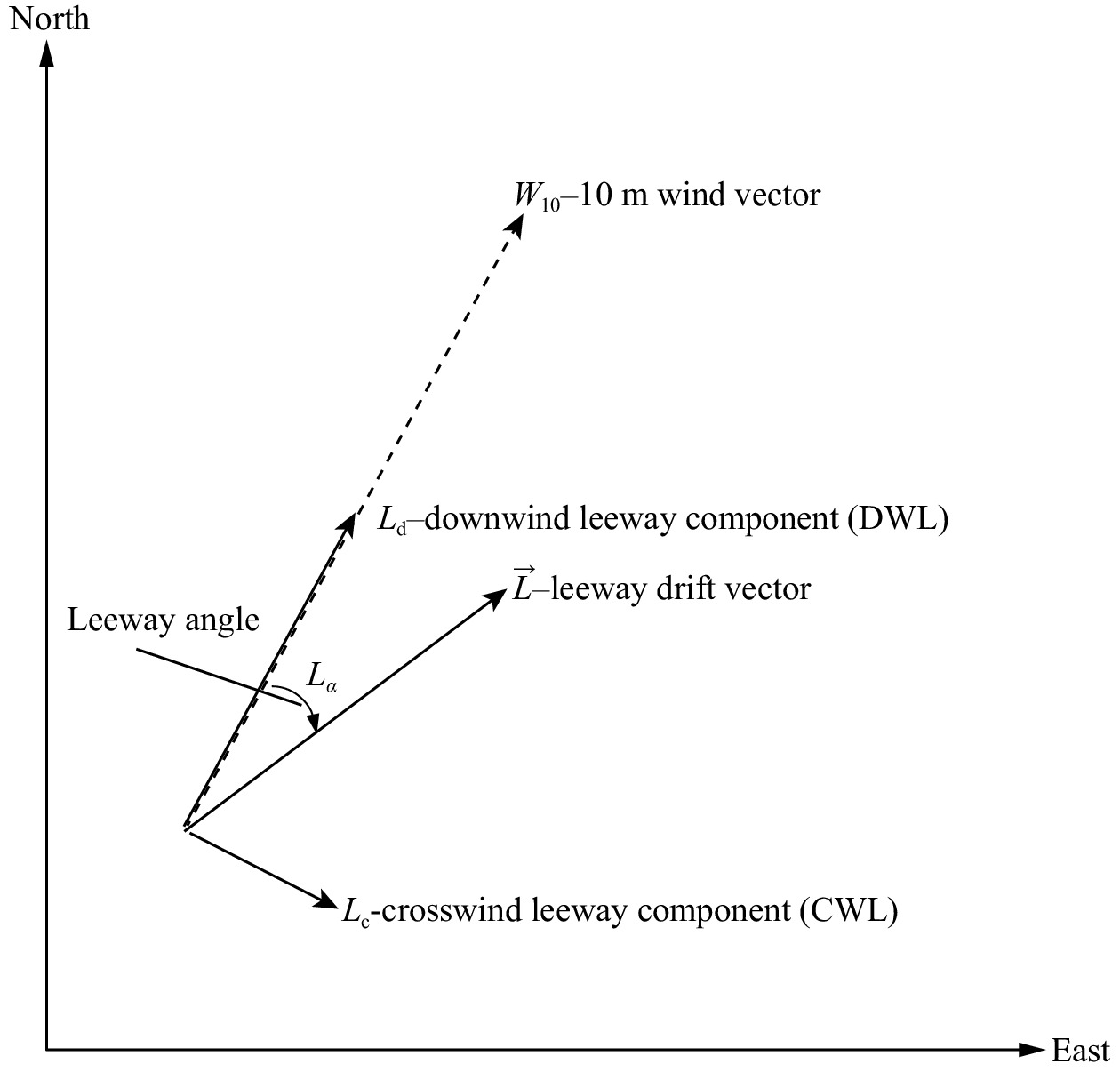
where $ {\overrightarrow{V}}_{{\rm{c}}} $ is the velocity of ambient current, including geostrophic current, tidal current, assorted baroclinic current, wind-induced current, etc. $ \overrightarrow {L} $ is the wind-induced leeway drift velocity generated by wind which is related to the shape and size of the objects. The observations show that a drifting object under the influence of the wind will diverge to some extent from the downwind direction, which is known as the wind-induced leeway angle, due to the interaction between the hydrodynamic effect of underwater part and the aerodynamic effect of the wind (Zhang et al., 2017). Due to the unstable angle between the direction of the wind-induced leeway and the wind at low wind speed, Allen and Plourde (1999) found that the best scheme to regress leeway $ \overrightarrow {L} $is to decompose it into downwind of the leeway component $ {L}_{{\rm{d}}} $ and crosswind leeway component $ {L}_{{\rm{c}}} $ (see Fig. 1, adapted from Allen and Plourde (1999)). More accurately, various experimental data show an almost linear relationship between wind speed W₁₀ and the downwind $ {L}_{{\rm{d}}} $ and the crosswind $ {L}_{{\rm{c}}} $ of the leeway components:

Figure  1.  The leeway $ \overrightarrow{L} $ of a drifting object consists of a DWL, $ {L}_{{\rm{d}}} $, and a CWL, $ {L}_{{\rm{c}}} $. The angle between the downwind direction and the leeway drift direction is termed the leeway angle, $ {L}_{\alpha } $.

DownLoad: Full-Size Img PowerPoint

here, $ {a}_{{\rm{d}}} $, $ {b}_{{\rm{d}}} $, $ {a}_{{\rm{c}}} $, and $ {b}_{{\rm{c}}} $ are regression coefficients. Field studies have been carried out to determine how different classes of objects respond to the wind, and the empirically derived coefficients for 63 categories of search objects compiled by the US Coast Guard are considered to estimate the leeway of the drifting object (Allen, 2005; Hackett et al., 2006; Breivik et al., 2012). Due to the stochastic changes in the sea surface wind field, the direction of the wind-induced leeway is uncertain and may be left or right of the local downwind direction. For a symmetrically shaped object, the wind-induced leeway velocity component is of equal magnitude to both sides of the drift. For a target with an asymmetrical shape, the wind-induced drift velocity components are of different magnitudes on both sides of the deviation, i.e., $ {a}_{{\rm{c}}} $ and $ {b}_{{\rm{c}}} $ take different values on both sides (Ni et al., 2010; Di Maio et al., 2016). In practice, there are errors in the sea surface wind forecast, and a random walk wind perturbation model is implemented to correct the wind data.

Following the assumptions and simplifications above, the trajectory model simplifies the calculation of the arc traced by the leeway vector and the sea surface current:

where $ {P}_{0} $ and $ {t}_{0} $ are the LKP and the falling time of the object. In addition to the errors of wind data and leeway mentioned above, the information we obtained about the LKP and the falling time of the object may be inaccurate. Thus, the Leeway model estimates the errors and uncertainties and to perform a Monte Carlo integration by rerunning the trajectory model multiple times with all relevant parameters perturbed to generate an ensemble, and the ensemble yields an estimate of the time evolving probability density function of the location of the search object, and its envelope defines the search area.

Based on the above model, we presented the Leeway-Trace model which transformed the traceability analysis of the target in real time and space into the trajectory prediction of the drifting object in virtual time and space. The Leeway model predicts the trajectory of the object in a time-increasing manner, while the Leeway-Trace model constructs the time series in virtual space-time that correspond to the inverse sequence in real space-time. For example, the start time of the traceability analysis in real space-time is 20:00 on May 8, 2019; we backtrack the drift trajectory of the object for the past 3 h, the corresponding start time of trajectory prediction in virtual space-time can be specified as 1:00 on January 1, 1900 (or any other arbitrary time), and the time series of the trajectory prediction are 2:00, 3:00, and 4:00 on January 1, 1900, which are assigned to the inverse time series of 19:00, 18:00 and 17:00 on May 8, 2019, respectively, for the traceability analysis in real space-time. The results of the trajectory prediction at the corresponding moments are taken as the results of the traceability analysis. The wind (10 m level) and the sea surface current used for the traceability analysis in real space-time are recorded as ${\overrightarrow{{V}}}_{1\mathrm{W}}$ and ${\overrightarrow{{V}}}_{1\mathrm{C}}$. ${\overrightarrow{{V}}}_{1\mathrm{W}}$ and ${\overrightarrow{{V}}}_{1\mathrm{C}}$ are generally obtained from numerical simulations (i.e., the numerical reanalysis data of wind and current). The wind and sea current velocities used for the prediction of virtual spatiotemporal drift trajectories are given as ${\overrightarrow{{V}}}_{2\mathrm{W}}$ and ${\overrightarrow{{V}}}_{2\mathrm{C}}$. The relationship can be expressed as follows:

The traceability analysis can be divided into the following three steps. In the first step, the virtual space-time of trajectory prediction is constructed, the start time and position of the object traceability analysis are converted to the falling time and LKP of the object trajectory prediction respectively, and the time series of the traceability are deserialized to obtain the time series of the trajectory prediction. The wind and current of the real space-time are reversed to obtain those of the virtual space-time. In the second step, trajectory prediction in virtual space-time is performed using the Leeway model. In the third step, the drift trajectory prediction results in the virtual space-time are converted to the traceability results in the real space-time.

3. Drifting buoy observation experiment in the northern SCS

We participated in the SCS Voyage Observation Program organized by the First Institute of Oceanography at the Ministry of Natural Resources on April 16–20, 2019, and conducted drifting buoy observation experiments. As shown in Fig. 2, a humanoid buoy and a spherical buoy were released in the experiment. The humanoid buoy mainly simulated the drifting motion of PIW, which was designed to imitate the shape, volume and weight of a human body wearing a survival suit. And it was equipped with a dedicated CLASS-B 10 receiver to automatically collect and send position information every 5 min. An additional small buoy was attached to the humanoid buoy, and it received position information by satellite. The spherical buoy was mainly used to measure the current velocity of the surface water and automatically collected and sent position information every 30 min, receiving information on the location and current velocity of the buoy by satellite. Table 1 shows the initial time and location of the two buoys and their positions after 10 days of drifting. The spherical buoy was released 5 h earlier than the humanoid buoy, and they were launched 78.71 km apart. Figure 3 shows that the spherical buoy first drifted to the north and then to the southwest. The humanoid buoy drifted northwest firstly and then southwest. There are some clockwise spiral features in the drifting trajectories of the two buoys.

Figure  2.  Photo of the spherical buoy (a) and the humanoid buoy (b).

DownLoad: Full-Size Img PowerPoint

Table  1.  Time and locations of the spherical buoy and the humanoid buoy

Buoy	Release time	Release location	Location after 10 days
Spherical	10:27, April 18	20°11.31'N, 116°18.18'E	20°26.36'N, 115°51.53'E
Humanoid	15:13, April 18	20°22.10'N, 115°34.47'E	20°15.06'N, 114°23.36'E

 | Show Table

DownLoad: CSV

Figure  3.  Drift trajectories of the spherical and humanoid buoys. The red area in the inset figure is the domain of the buoy drift observations.

DownLoad: Full-Size Img PowerPoint

4. Numerical simulations of the sea current in the SCS

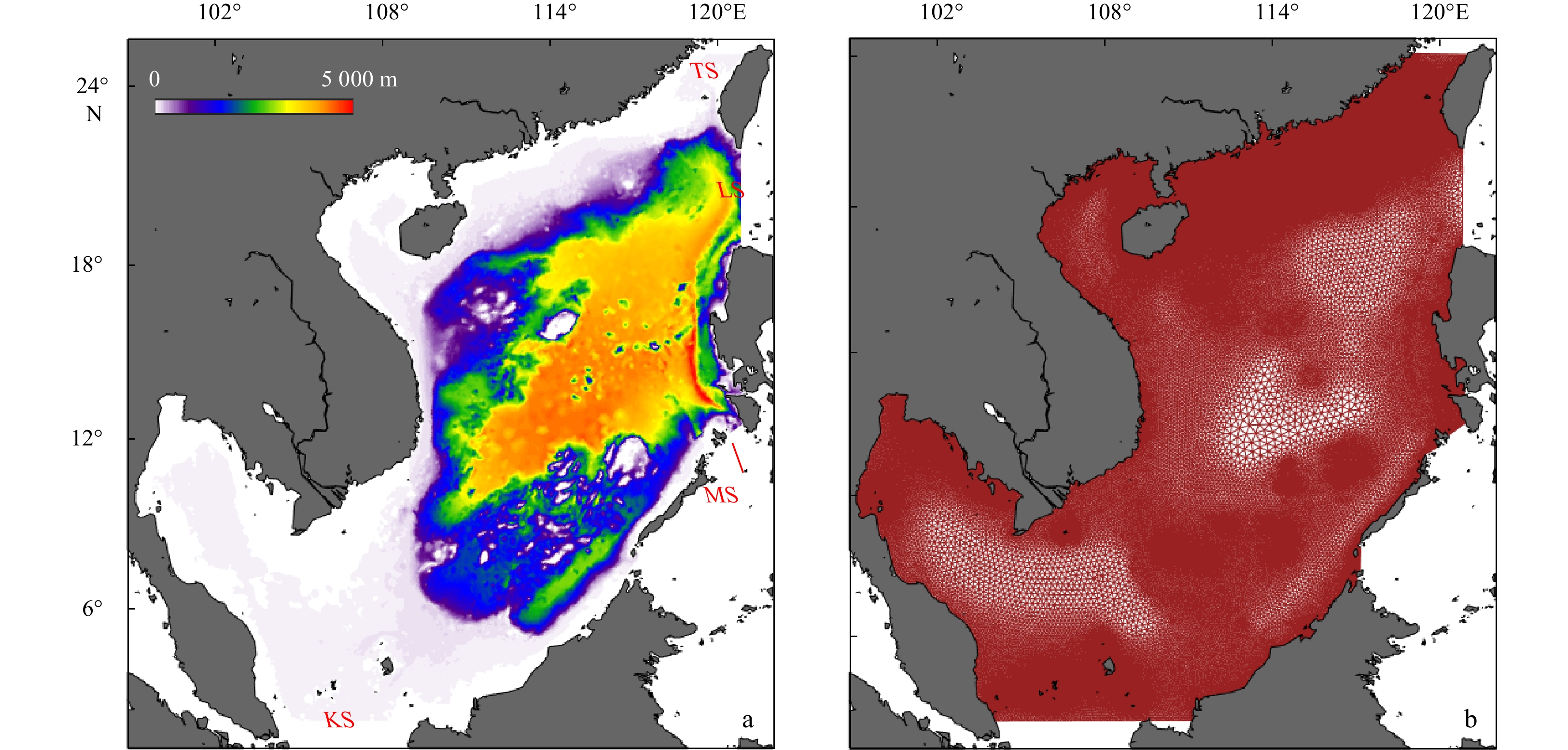
FVCOM is an unstructured-grid, finite-volume, free-surface, three-dimensional primitive equations community ocean model (Chen et al., 2003). Its finite-volume approach combines the best of finite-element methods for geometric flexibility and finite-difference methods for simple discrete structures and computational efficiency. The model domain extends from 1°N to 25°N in the north−south direction, and from 99°E to 121°E in the east−west direction (Fig. 4a). With 71 989 unequally spaced nodes and 140 260 elements, the horizontal resolution is typically 6–7 km over the shelf and 4–5 km along the coast and shelf edge (Fig. 4b). A generalized terrain-following coordinate was designed to resolve the free surface and bottom topography and 51 levels were nonuniformly distributed in the vertical direction. Based on Courant-Friedrichs-Levy numerical stability condition, model equations were solved with an integration time step of 3 s for the external mode and an internal to external mode ratio of 10.

Figure  4.  Topography in the South China Sea, showing Luzon Strait (LS), Taiwan Strait (TS), Mindoro Strait (MS) (a), and Karimata Strait (KS) and unstructured mesh for the ocean model (b). Color contour of a represents bathymetry.

DownLoad: Full-Size Img PowerPoint

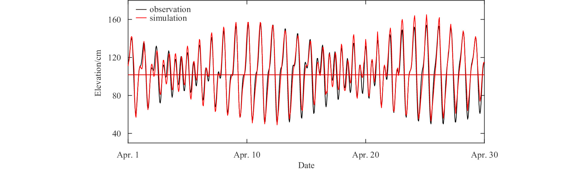
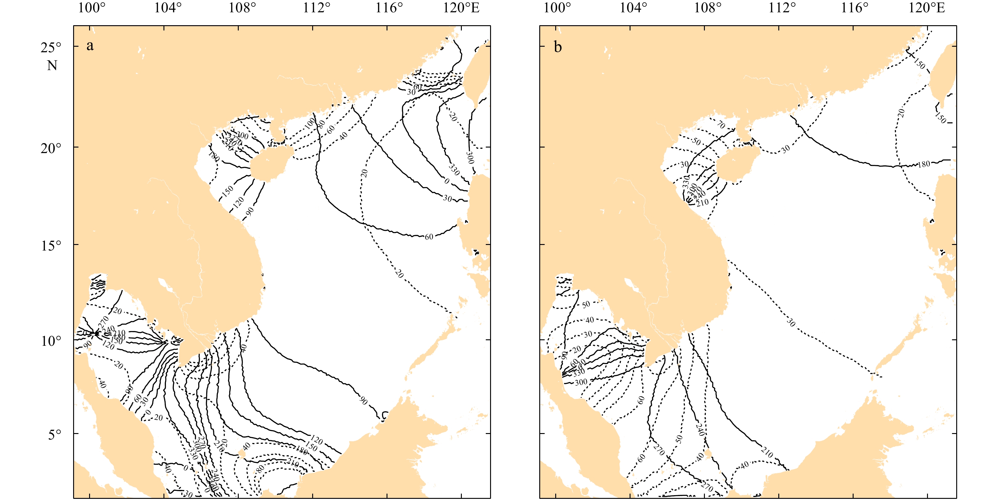
Numerical simulations of astronomical tides were first performed. The model tidal level and velocity were initialized from zero. Along the open boundaries, the tidal elevations for the eight major semi-diurnal (M₂, S₂, K₂ and N₂) and diurnal (K₁, O₁, N₁ and Q₁) constituents provided by a global inverse tidal model (Egbert and Erofeeva, 2002) were specified in time series. The temperature and salinity fields were set to constant. The astronomical tide simulations were performed from March 1 to April 30, 2019, and the results of the latter 30 days were taken for the harmonic analysis of tides. Figure 5 shows the simulated cotidal chart of the M₂ and the K₁ tidal constituents respectively. One branch of M₂ propagates northeastward into the Taiwan Strait, but its propagation is hindered by southward tidal waves, and the isophase becomes very dense with a sudden increase in amplitude. The K₁ tidal constituent spreads from the Pacific Ocean to the SCS through the Luzon Strait and the Taiwan Strait, there is no northward branch in the Taiwan Strait, which is different from the semidiurnal tide. After entering the SCS, the K₁ tidal constituent mainly spreads in a southwest direction. The propagation characteristics of the S₂, K₂ and N₂ tidal constituents are similar to those of the M₂ tidal constituent with smaller amplitudes than M₂, while the propagation characteristics of the O₁, P₁ and Q₁ tidal constituents are similar to those of the K₁ tidal constituent with smaller amplitudes than K₁. Overall, the harmonic constant distribution of the numerical simulations in this paper is similar to those of Ding (1986), and Gao et al. (2014). We collected the harmonic constants induced from tide table data of 21 stations in the SCS. Table 2 shows the error statistics of the simulation and tidal table data for the M₂, S₂, K₁ and O₁ tidal harmonic constants, with mean absolute errors of 5.52 cm, 4.89 cm, 4.28 cm and 4.30 cm for the amplitudes and 9.01°, 11.74°, 9.21° and 10.88° for the phases, respectively. The hydrological station nearest to the drift buoy experimental area is Dongsha Station, which is located at 20°42′N, 116°43′E. Figure 6 gives the tide levels of the tidal table and numerical simulation at Dongsha Station during April 1–30, 2019. The figure demonstrates that there is good agreement between them, and the average absolute error is 11.7 cm.

Figure  5.  Calculated co-tidal lines in the South China Sea (SCS). The co-tidal chart for M₂ (a) and K₁ (b) in the SCS. Dashed line is for amplitude (unit: cm), and solid line is for phase lag (unit: (°)).

DownLoad: Full-Size Img PowerPoint

Table  2.  Error statistics of astronomical tide simulation

Location	M2			S2			K1			O1
	ΔH/cm	Δg/(°)		ΔH/cm	Δg/(°)		ΔH/cm	Δg/(°)		ΔH/cm	Δg/(°)
24°27'N, 118°04'E	8.7	15.4		6.3	17.5		4.9	13.7		3.8	9.2
23°44'N, 117°32'E	5.6	12.5		4.3	13.9		3.3	11.9		4.1	8.5
23°27'N, 116°51'E	7.1	9.3		5.7	9.8		6.5	13.7		2.4	5.9
22°36'N, 114°32'E	6.4	8.5		6.5	10.1		3.4	7.6		3.0	7.1
21°30'N, 110°24'E	3.5	5.3		8.1	12.4		4.7	9.0		5.1	11.3
21°29'N, 109°05'E	6.4	10.2		4.2	14.8		5.3	10.1		4.6	13.8
20°13'N, 110°07'E	5.8	8.8		2.9	11.2		3.4	8.5		6.2	11.9
18°24'N, 109°30'E	4.3	7.6		3.6	12.3		2.5	5.4		4.1	10.2
21°36'N, 109°35'E	5.4	10.1		2.7	9.4		3.3	6.1		4.2	10.5
20°01'N, 110°17'E	6.2	10.3		4.8	11.3		5.1	8.0		5.5	13.1
19°06'N, 108°37'E	6.7	11.3		6.5	10.2		4.6	8.5		4.4	10.8
22°36'N, 120°17'E	3.5	6.0		4.2	12.4		3.4	7.8		4.1	10.0
23°33'N, 119°32'E	6.1	8.6		5.3	12.3		5.6	10.2		5.4	11.5
16°50'N, 112°20'E	6.9	11.2		3.4	8.9		6.0	11.4		6.1	17.6
11°27'N, 114°19'E	3.6	5.4		4.6	13.1		4.1	8.5		4.5	14.1
9°32'N, 112°53'E	5.3	9.8		3.8	9.2		4.8	9.8		3.9	10.8
10°18'N, 123°55'E	4.6	7.5		6.2	12.5		3.4	7.6		4.1	11.3
5°21'N, 103°08'E	7.2	8.8		4.5	11.2		5.2	10.0		4.5	12.1
2°31'N, 101°47'E	5.6	8.5		6.2	10.4		3.5	7.4		3.1	9.7
1°16'N, 103°49'E	3.5	6.7		4.1	12.1		3.2	8.5		4.0	10.5
1°20'N, 104°24'E	3.4	6.2		4.7	11.5		3.7	9.7		3.3	8.6
Note: ΔH represents the absolute error between the simulation and the tidal table data of the amplitude for the tidal constituent; Δg represents the absolute error between the simulation and the tidal table data of the phase for the tidal constituent.

 | Show Table

DownLoad: CSV

Figure  6.  Comparison of elevations between simulation and observation.

DownLoad: Full-Size Img PowerPoint

Based on the numerical simulation of the astronomical tide, a coupled tide-circulation numerical simulation was performed. The model was forced by winds and heat fluxes at the sea surface. Spatially variable wind speed, short-wave heat flux, long-wave heat flux, latent heat flux and sensible heat flux from NCEP Climate Forecast System Reanalysis (CFSR) were used over the entire computational domain. CFSR is the third-generation global reanalysis, using the Coupled Forecast System (CFS) model, with output 4 times daily. The temperature, salinity and nontidal circulation conditions for the open boundaries were derived from the (1/12)° daily HYCOM reanalysis data. The initial variables (i.e., sea surface height, velocity, temperature and salinity) were also generated from the HYCOM data on March 1, 2019. For the surface forcing, the 6-hourly data were derived from the CFSR model. The model was integrated from March 1 to March 31, 2019. The model was integrated from March 1 to March 31, 2019. Then we restarted the model from April 1 to 30, 2019. Tidal levels and vectors of the FVCOM output were merged into the initial condition and the open boundaries. Other settings were the same as above. The results from April 18–28 were adopted for the traceability analysis of the drifting buoys.

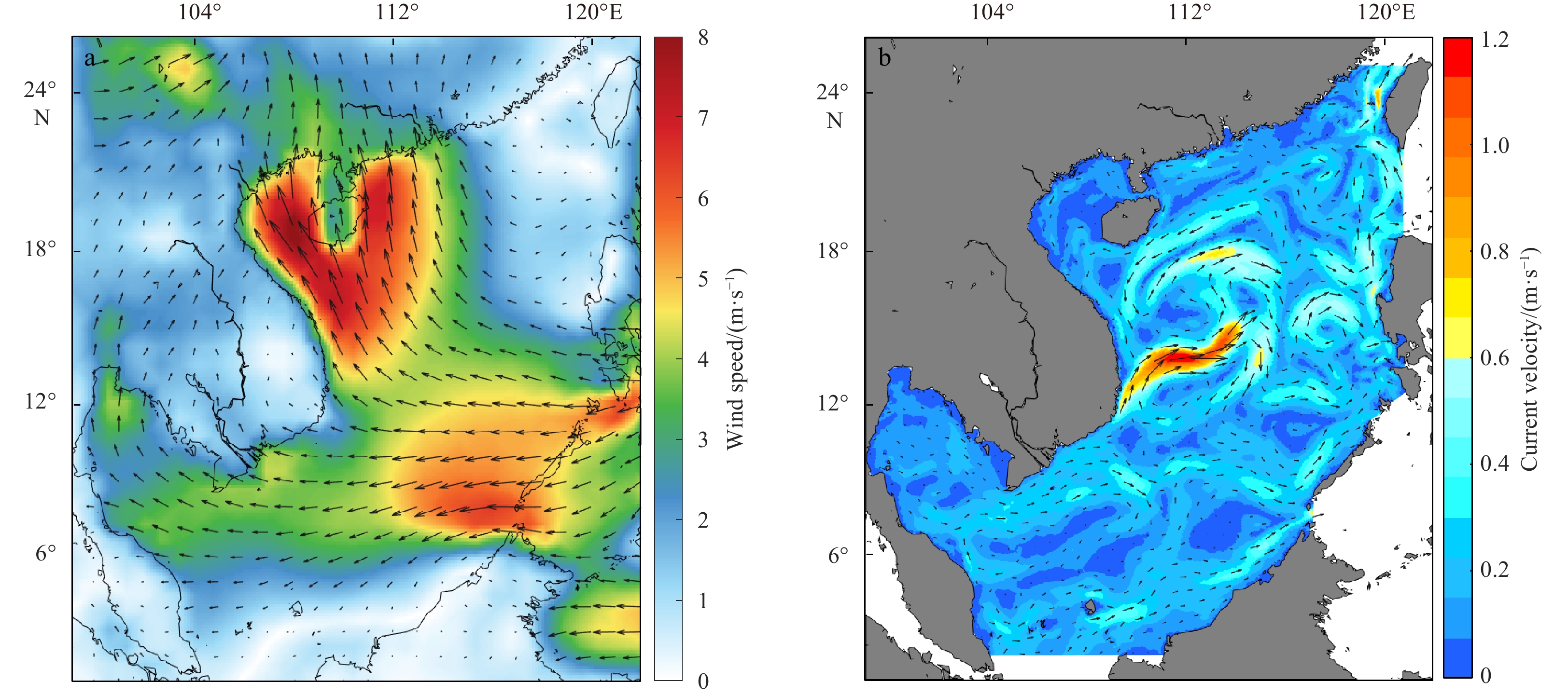
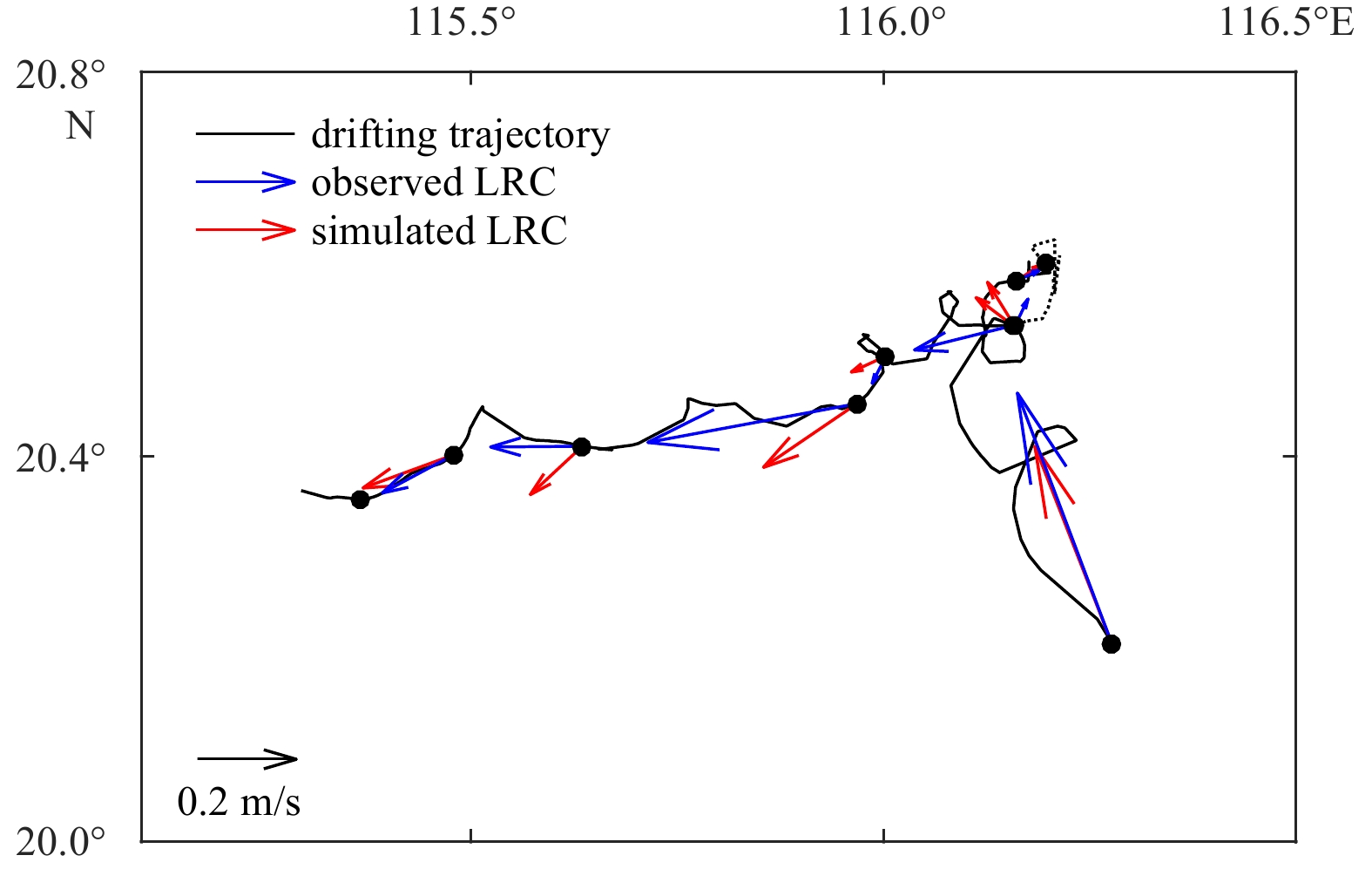
Figure 7a shows the mean wind during April 18–28 in the drifting buoy observation experiment. The wind speed distribution in the northern SCS (north of 19°N) during this period was 1–8 m/s, and the south wind was dominant. Figure 7b is the simulated average current field from April 18 to 28. From Fig. 7b, we can see that the overall velocity in the SCS was relatively weak, but there was a strong offshore current along the coast of Vietnam. There was a distinct westward current in the experimental area, which is consistent with the overall movement of the humanoid and spherical buoys. The drifting trajectory of the spherical buoy tracked by the satellite was divided into nine segments according to the two cycles of the M₂ tidal constituents as time intervals, and the observed Lagrangian residual current (LRC) were obtained by using the drift trajectory of each segment. The signal of the circular buoy in the fourth segment was unstable, and the received position information was rather disordered, which was not used to calculate the observed LRC. At the initial position and moment of each trajectory, the simulated current was used for the Lagrangian particles tracking within two M₂ tidal periods, then the simulated LRC can be obtained. Figure 8 presents the comparison between the observed and simulated LRCs. The average of the observed LRC velocity is 18.84 cm/s, the average absolute error between the simulated and observed LRC velocities is 3.76 cm/s, and the average error of the LRC direction is 33.12°. The observed and simulated LRCs generally agree, but there are still errors in the numerical simulation. In order to obtain the better current velocity for traceability analysis, the observed velocity of the spherical buoy is assimilated into the model, and the assimilation scheme was the Kalman filter method.

Figure  7.  The average velocity of wind (a) and sea surface current (b) in the South China Sea during April 18–28, 2019.

DownLoad: Full-Size Img PowerPoint

Figure  8.  The observed and simulated Lagrangian residual current (LRC) of the spherical buoy.

DownLoad: Full-Size Img PowerPoint

5. The traceability analysis of the humanoid buoy

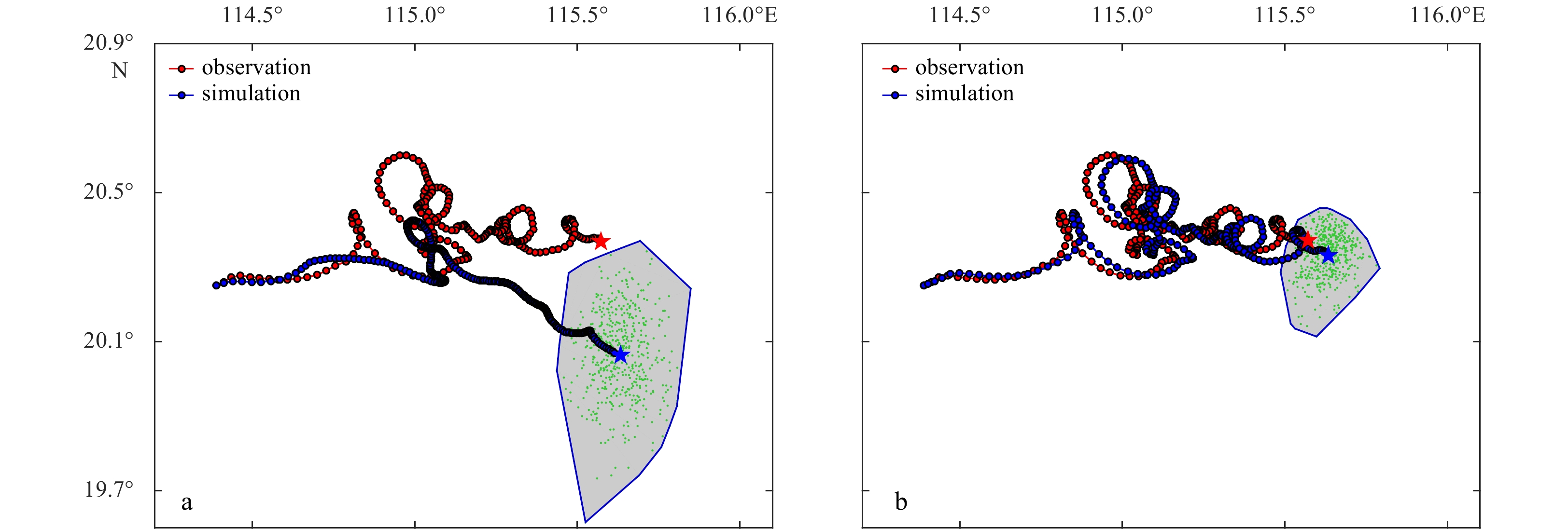
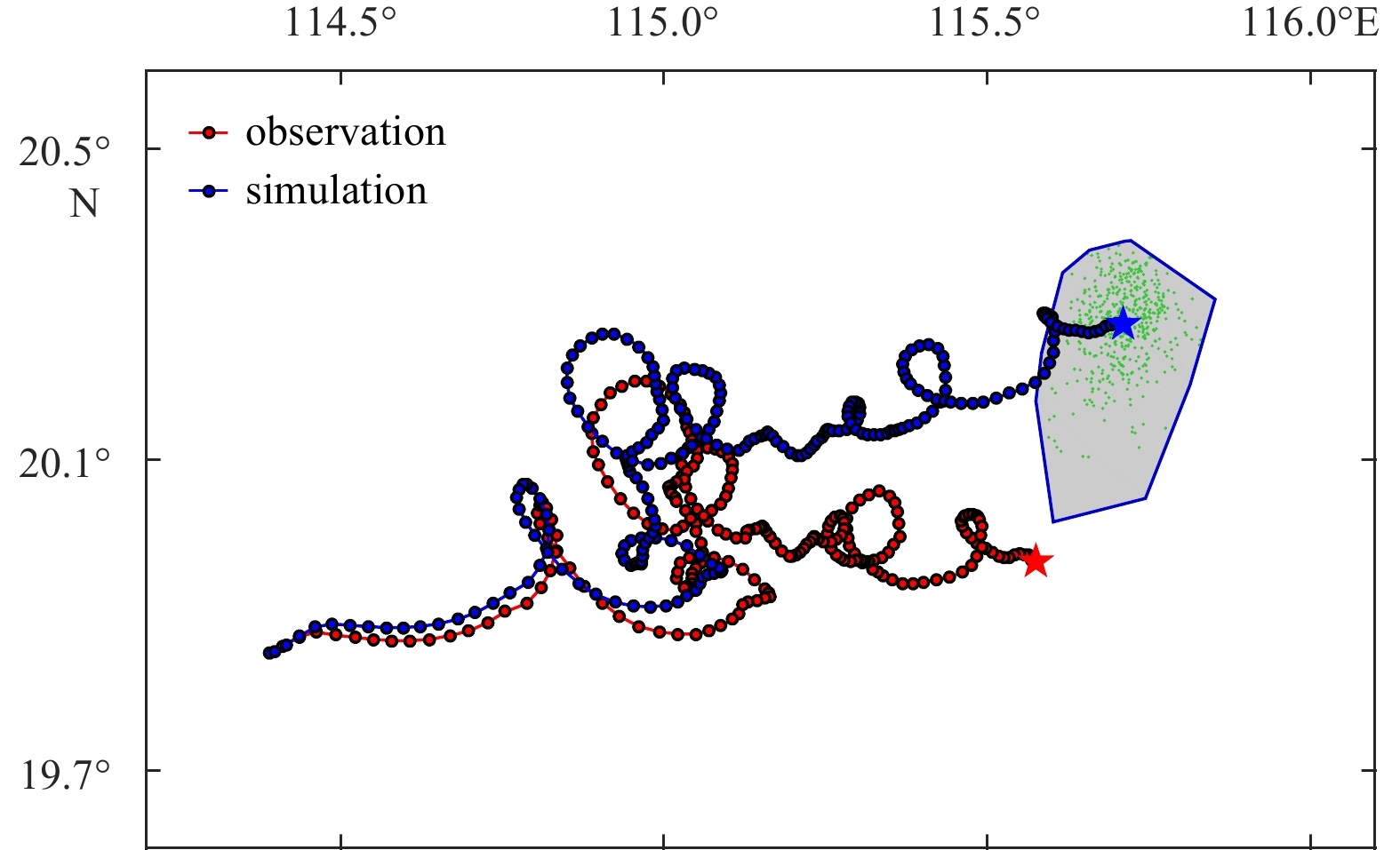
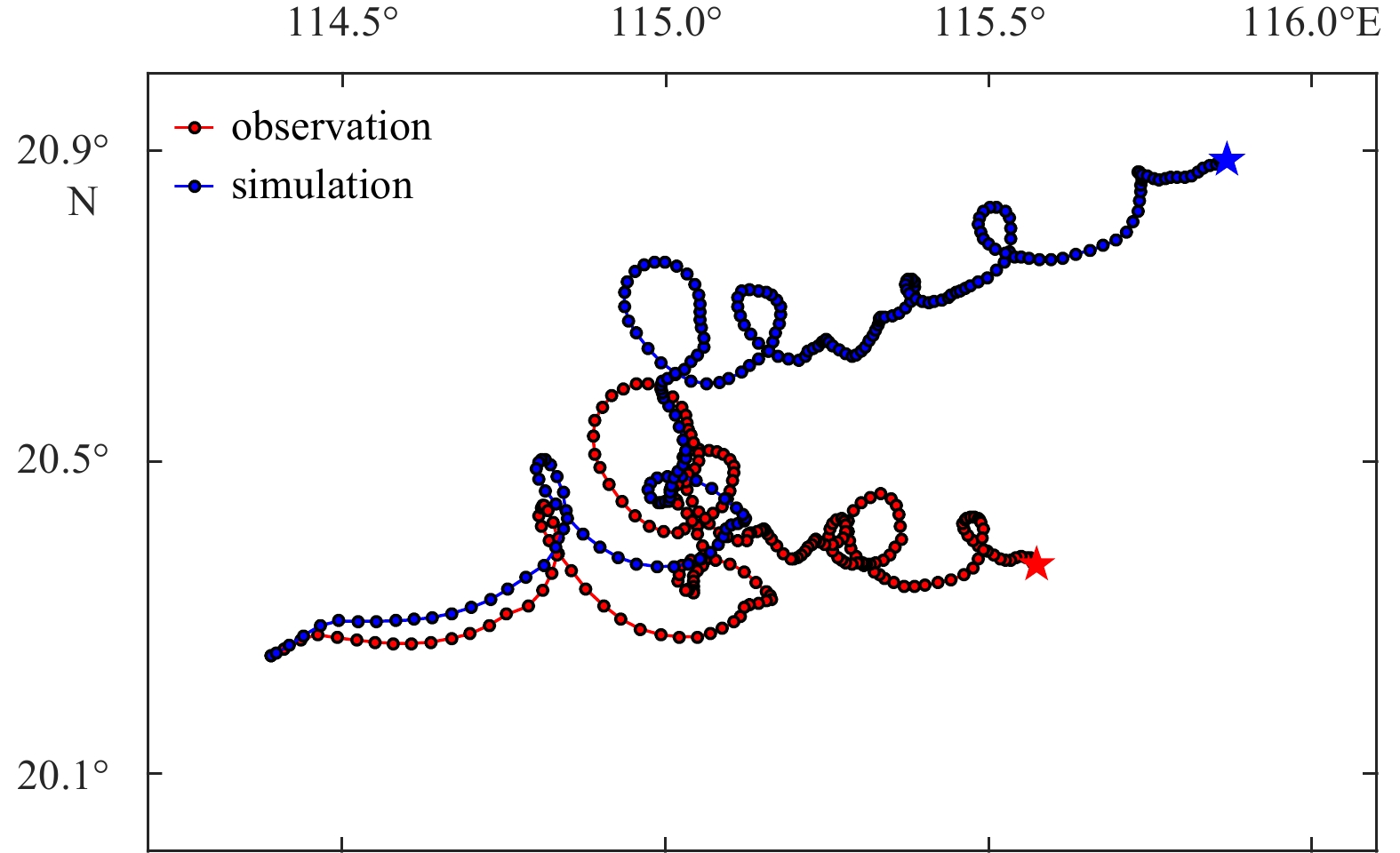
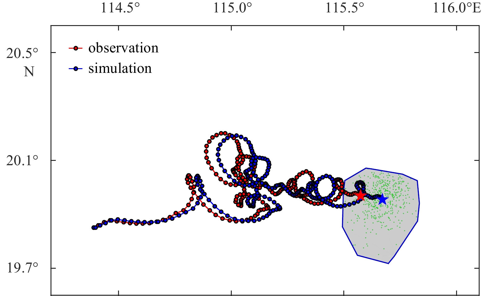
Two experiments were designed to examine the ability of the Leeway-Trace model in tracing the humanoid buoy. Since the release time and location of the humanoid buoy in this observation are very accurate, the initial time of the traceability was taken as 15:13 of April 28, and the possible deviation of the release location information was only 10 m. Five hundred particles were released in an area of 10 m radius to trace humanoid buoy back over the past 10 days. The CASE01 experiment adopted the coupled tide-circulation numerical simulation without assimilating the observed sea current, and the wind data were from CFSR. The settings of CASE01 were used for CASE02 except that the observed current was assimilated into the model. Figure 9 present the results of the traceability analysis from CASE01 and CASE02, respectively. At the end of the traceability analysis at April 18 15:13, the positions of 500 particles were given, the convex hull of these particles is used as the most likely distribution area of the buoy, and the average position of these particles is used as the most likely location of the humanoid buoy. At other moments in the traceability analysis, only the average positions of the 500 particles were given as the historical trajectory of the humanoid buoy. As shown in Fig. 9, the trajectories of CASE01 and CASE02 were relatively close to the observation during the first 24 h. Then the trajectory of CASE01 and the observed one differed, and the former was basically on the south side of the latter. When tracing back to 15:13 of April 18, the central location of the CASE01 was 20.07°N, 115.61°E, and it was located 35.30 km southeast of real placement. The possible distribution area size of CASE01 was 1571.69 km², which did not include the observed location of the humanoid buoy. Figure 9b shows the tracking trajectory of CASE02 as deviating eastward from the observed trajectory after 18 h, and when traced back to 15:13 of April 18, the central position of CASE02 was 20.34°N, 115.59°E, and it was located east of the real placement, 7.54 km apart. And the possible distribution area size of CASE02 was 225.40 km², which included the actual releasing location of the humanoid buoy.

Figure  9.  Particle trajectories of CASE01 (a) and CASE02 (b). The observed trajectory of the humanoid buoy is shown as a red line, while the simulated result of the Leeway-Trace model is shown as a blue line. The red star indicates the position at which the humanoid buoy was deployed, while the blue star indicates the position of the final center position from the traceability analysis. These green dots represent the traceable position of 500 particles at 15:13 on April 18, and the possible distribution of traceability is indicated by the convex hull polygon.

DownLoad: Full-Size Img PowerPoint

By comparing CASE01 and CASE02, the assimilation of observed sea currents has little influence on the traceability results for the short-term (1 d) traceability analysis, but for the long-term (2–10 d) traceability analysis, the assimilation of observed sea currents can significantly improve the accuracy of the traceability analysis. There may be some small eddies in the SCS, which affect the movement of the buoys. The model above is not so good for small eddies simulation, thus there are still some errors in the numerical simulation of sea current, which cause the differences of the traceability analysis without data assimilation and the actual characteristics of drifting trajectory to be far from each other. Therefore, it is very important to strengthen the observation and assimilation of the sea current for the traceability analysis in maritime accident.

6. Impacts of wind and tide on the traceability analysis

As mentioned in the introduction, the water particle trajectory tracking in marine scientific research just considers the effect of sea current, while the Leeway-Trace model considers both the effects of sea current and the wind-induced leeway drift. To further verify the effect of wind-induced sea surface current and leeway on the traceability analysis, three sensitive experiments were designed. Moreover, it is generally believed that tides are weaker in most of the SCS away from the coast. We also designed a sensitive experiment to discuss the impact of tide on the traceability analysis.

6.1 Impacts of wind on the traceability analysis

The wind-induced surface current was simulated by the FVCOM model. Figure 10 show the wind rose and surface wind-induced current rose in the buoy experimental area from April 18 to 28, 2019 respectively. Both the wind and wind-induced current are averaged over all grid points in the area, with a time interval of 6 h for the wind and 1 h for the wind-induced sea surface current. From Fig. 10a, we see that the south, southeast, and southwest winds occurred in 56.9%, 10.6%, and 5.98% of the time, respectively, with an average wind speed of 4.12 m/s, and east and northeast winds occurred in 23.1% and 3.99% of the time, respectively, with an average wind speed of 4.33 m/s. In Fig. 10b, the surface wind-induced currents to the north, northeast, and east occurred in 23.74%, 45.99% and 8.69% of the time, respectively, with an average speed of 7.88 cm/s. And those to the west and northwest occurred 12.13% and 7.88% of the time, respectively, with an average speed of 2.66 cm/s. Overall, the experimental area is dominated by southerly winds and wind-generated sea flows pointing to the northeast.

Figure  10.  Wind rose (a) and wind-induced current rose (b) of the northern South China Sea from April 18 to 28, 2019.

DownLoad: Full-Size Img PowerPoint

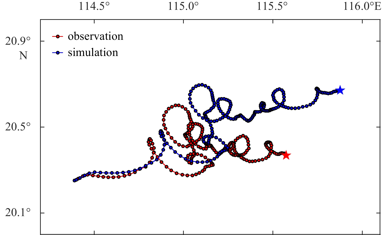
We designed CASE03, which did not consider wind-induced leeway drift, while the other settings were the same as those in CASE02. The traceability analysis results of CASE03 are shown in Fig. 11. The 500 particles for the traceability analysis were not dispersed due to the absence of possible errors in wind speed and randomness in the direction of the wind-induced leeway drift. The particles are still distributed within a 10 m radius circle at the end of the traceability analysis.

Figure  11.  Result of the particle trajectory in CASE03. The observed trajectory of the humanoid buoy is shown as a red line, while the simulated result of the Leeway-Trace model is shown as a blue line. The red star indicates the position at which the humanoid buoy was deployed, while the blue star indicates the position of the final center position from the traceability analysis.

DownLoad: Full-Size Img PowerPoint

The traceability analysis path of CASE03 was closer to the humanoid buoy observation in the first 30 h and then gradually shifted northeast of the observation. At 15:13 of April 18, the center position of the CASE03 was 20.59°N, 115.80°E, which was located northeast of the observed location and the analysis results of CASE02, with distances of 34.88 km and 36.12 km, respectively. The results were equivalent to the drift prediction in virtual space-time, so that the difference between the results of CASE02 and CASE03 can be explained by the corresponding prediction of drift trajectories in virtual space-time. The winds in real space-time in CASE02 were predominantly southerly, so those for the drifting trajectory prediction in virtual space-time correspond to northerly winds. CASE03 removed the effect of the wind-induced leeway drift, thus the drifting trajectory prediction in virtual space-time has no effect of northly wind, so the result is more northerly than the that of CASE02.

We designed CASE04 to disregard the effect of wind-induced current on the traceability analysis. It deducted the wind-induced current from the current used in CASE02, and the other scenarios were not changed. The results of CASE04 are shown in Fig. 12, and the traced path is closer to the observation in the first 78 h, then it is gradually shifted to northeast of the observation. At 15:13 of April 18, the CASE04 results were centered at 20.70°N, 115.75°E, on the northeast side of the humanoid buoy placement location and the CASE02 analysis results, and at distances of 36.12 km and 44.68 km from the buoys, respectively. The difference between the traced results of CASE04 and CASE02 reveals the effect of wind-induced current with a physical interpretation similar to the effect of the wind-induced leeway drift above.

Figure  12.  Results of the particle trajectory in CASE04. The observed trajectory of the humanoid buoy is shown as a red line, while the simulated result of the Leeway-Trace model is shown as a blue line. The red star indicates the position at which the humanoid buoy was deployed, while the blue star indicates the position of the final center position from the traceability analysis. These green dots represent the traceable position of 500 particles at 15:13 on April 18, and the possible distribution of traceability is indicated by the convex hull polygon.

DownLoad: Full-Size Img PowerPoint

Additionally, we designed CASE05 without the effects of wind-induced current and wind-induced leeway drift. The traceability analysis results of CASE05 are shown in Fig. 13. The traced path in the first 78 h is relatively close to the observation, then the traced position is gradually shifted northward to the observation. At 15:13 of 18 April, the traceability results of CASE05 were centered at 20.89°N, 115.87°E, at distances of 66.01 km and 68.19 km in the northeast direction of the observation and the CASE02 traceability results respectively.

Figure  13.  Results of the particle trajectory in CASE05. The observed trajectory of the humanoid buoy is shown as a red line, while the simulated result of the Leeway-Trace model is shown as a blue line. The red star indicates the position at which the humanoid buoy was deployed, while the blue star indicates the position of the final center position from the traceability analysis.

DownLoad: Full-Size Img PowerPoint

The difference in locations between CASE02 and the observations at the time the buoy was launched was only 7.54 km, and the errors of CASE03 and CASE04 were 4.63 and 4.79 times of that in CASE02, respectively. It is shown that the lack of wind-induced current and leeway drift almost equally increased the traceability analysis error. CASE05 does not consider either wind-induced leeway drift or wind-induced current, and the error of the traceability analysis reaches 8.75 times of that in CASE02, the wind has an important influence on the traceability analysis in the SCS.

6.2 Impact of tidal currents on traceability analysis

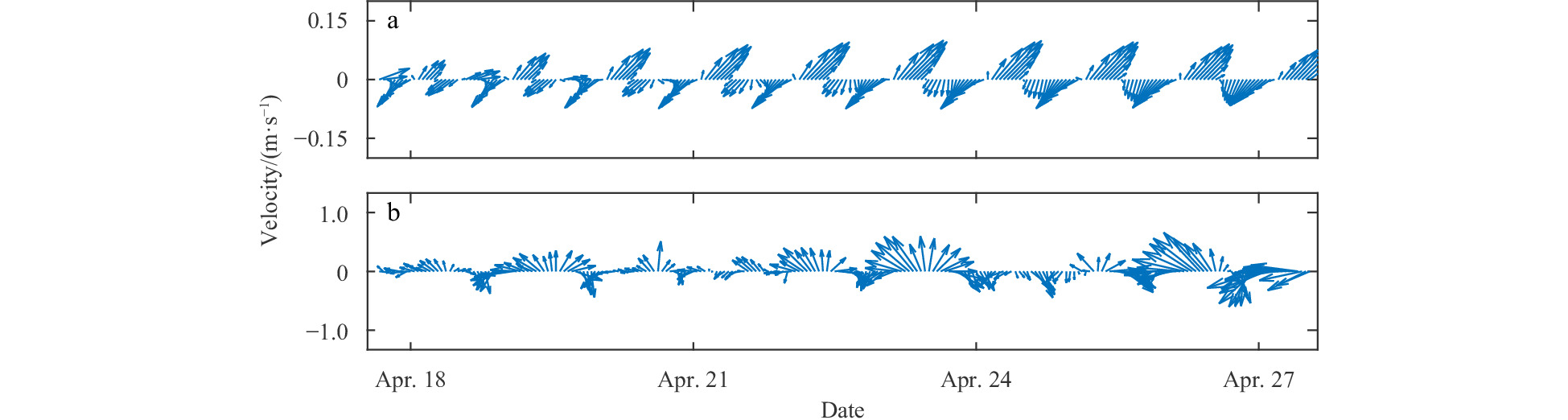
Figure 14a gives the hour-by-hour tidal currents from April 18 to 28 at 20.6°N, 115.3°E inside the buoy observation experiment area, in which the data are derived from the astronomical tide numerical simulations presented in Section 4 of this paper. Figure 14b shows the residual currents by subtracting the tide constituent from the currents used in CASE02. The average velocity of tide is 6.19 cm/s, the average velocity of the residual currents is 44.05 cm/s, it is obvious that the tidal currents are much weaker than the residual currents. We designed CASE06, which subtracted the tidal currents from the current used in CASE02, and the rest of the scenario is same as that in CASE02. Figure 15 shows the results of the traceability analysis of CASE06. The traced position at 15:13 of April 18 was 20.36°N, 115.67°E, which is northeast to the actual buoy placement and the trace result of the CASE02 with distances of 16.10 km and 15.45 km, respectively. The error of traceability analysis of CASE06 increased by 104.91% compared with CASE02. It is shown that the influence of tidal currents on the traceability analysis of buoys cannot be ignored even in the area with weak tidal currents.

Figure  14.  The tidal currents (a) and residual currents (b) at 20.6°N, 115.3°E from April 18 to 28, 2019.

DownLoad: Full-Size Img PowerPoint

Figure  15.  Results of the trajectory in CASE06. The observed trajectory of the humanoid buoy is shown as a red line, while the simulated result of the Leeway-Trace model is shown as a blue line. The red star indicates the position at which the humanoid buoy was deployed, while the blue star indicates the position of the final center position from the traceability analysis. These green dots represent the traceable position of 500 particles at 15:13 on April 18, and the possible distribution of traceability is indicated bythe convex hull polygon.

DownLoad: Full-Size Img PowerPoint

7. Conclusions

In this paper, we proposed a method for traceability analysis in real space-time using drift trajectory prediction in virtual space-time, by which the Norwegian drifting trajectory prediction model (Leeway model) was developed to a traceability analysis model of Leeway-Trace. In the new model, the sea current, the wind-induced leeway drift (including the differences in leeway coefficients of objects, uncertainties in the direction of leeway angle, errors in wind data) and the error of the initial traceability information are in consideration.

Using the observed data of drifting buoys in the northern SCS during April 2019, the traceability analysis of a humanoid buoy by the Leeway-Trace model were made, in which the forces of sea current and wind were from the FVCOM model and the CFSR respectively. The short-term (1 d) traceability analysis was in good agreement with the observations, and the assimilation of the sea current observations had little effect on the traced results. But for the long time (2–10 d) traceability analysis, the results were also good if the observed sea currents were assimilated into force data, otherwise the errors significantly increased. Additionally, we designed some sensitive experiments to discuss the effects of wind and tidal current on traceability analysis. The wind has an important influence on the traced results, with the effects of wind-induced current and leeway drift being nearly equal. The tidal currents in the area of the buoy experiment were weak, but the influence of tides on the traced results could not be ignored. In the SCS, tidal currents are stronger near many coastal islands, and their influence on the traceability analysis is noteworthy.

Acknowledgements

We are very thankful to the First Institute of Oceanography at the Ministry of Natural Resources for organizing the SCS Voyage Observation Program, the National Ocean Partnership Program (NOPP) for sharing the reanalysis ocean data of HYCOM and the National Centers for Environmental Prediction (NCEP) for releasing the reanalysis meteorological product.