Kui Zhang, Ping Geng, Jiajun Li, Youwei Xu, Muhsan Ali Kalhoro, Mingshuai Sun, Dengfu Shi, Zuozhi Chen. Influences of fisheries management measures on biological characteristics of threadfin bream (Nemipterus virgatus) in the Beibu Gulf, South China Sea[J]. Acta Oceanologica Sinica, 2022, 41(3): 24-33. doi: 10.1007/s13131-021-1925-9
Citation:
Kui Zhang, Ping Geng, Jiajun Li, Youwei Xu, Muhsan Ali Kalhoro, Mingshuai Sun, Dengfu Shi, Zuozhi Chen. Influences of fisheries management measures on biological characteristics of threadfin bream (Nemipterus virgatus) in the Beibu Gulf, South China Sea[J]. Acta Oceanologica Sinica, 2022, 41(3): 24-33. doi: 10.1007/s13131-021-1925-9
Kui Zhang, Ping Geng, Jiajun Li, Youwei Xu, Muhsan Ali Kalhoro, Mingshuai Sun, Dengfu Shi, Zuozhi Chen. Influences of fisheries management measures on biological characteristics of threadfin bream (Nemipterus virgatus) in the Beibu Gulf, South China Sea[J]. Acta Oceanologica Sinica, 2022, 41(3): 24-33. doi: 10.1007/s13131-021-1925-9
Citation:
Kui Zhang, Ping Geng, Jiajun Li, Youwei Xu, Muhsan Ali Kalhoro, Mingshuai Sun, Dengfu Shi, Zuozhi Chen. Influences of fisheries management measures on biological characteristics of threadfin bream (Nemipterus virgatus) in the Beibu Gulf, South China Sea[J]. Acta Oceanologica Sinica, 2022, 41(3): 24-33. doi: 10.1007/s13131-021-1925-9
South China Sea Fisheries Research Institute, Chinese Academy of Fishery Sciences, Guangzhou 510300, China
2.
Key Laboratory for Sustainable Utilization of Open-sea Fishery, Ministry of Agriculture and Rural Affairs, Guangzhou 510300, China
3.
Southern Marine Science and Engineering Guangdong Laboratory (Guangzhou), Guangzhou 511458, China
4.
Faculty of Marine Sciences, Lasbela University of Agriculture, Water and Marine Sciences, Uthal 90150, Pakistan
Funds:
The National Key R&D Program of China under contract No. 2018YFD0900906; the National Natural Science Foundation of China under contract No. 31602157; the Key Special Project for Introduced Talents Team of Southern Marine Science and Engineering Guangdong Laboratory under contract No. GML2019ZD0605; the Central Public-Interest Scientific Institution Basal Research Fund under contract Nos 2020TD05 and 2021SD01.
Long-term variations in population structure, growth, mortality, length at median sexual maturity, and exploitation rate of threadfin bream (Nemipterus virgatus) are reported based on bottom trawl survey data collected during 1960–2012 in the Beibu Gulf, South China Sea. Laboratory-based analyses were conducted on 16791 individuals collected quarterly in eight different sampling years. Average body length, estimated asymptotic length, and percentage of large individuals have decreased significantly with the growth of marine catch and fishing power, indicating individual miniaturization of this fish species. Estimated exploitation rates indicate that the N. virgatus stock in the Beibu Gulf was moderately exploited in 1960 and 1962 and overexploited after 1992. This stock was taking a good turn in status in 2012, with the lowest exploitation rate since 1992 and ceased downward trend in length indexes. These results suggest that management measures to reduce fishing pressure may have a positive influence on the biological characteristics of this commercial fish species. Biological characteristics of most commercial fish species have phenotypic plasticity and might change over years in response to fisheries management. Therefore, attentions should be paid on variations in fish biological characteristics, when evaluating the effectiveness of current measures to control the total catch for all fisheries.
Coastal fisheries provide a major source of food and livelihoods for inhabitants of coastal areas. The total catch of coastal fisheries is more than 5×10⁷ t annually, accounting for about half of global marine landings (Palomares and Pauly, 2019). However, there are still catch shortfalls in developed or rapidly developing countries due to the growing popularity of seafood (Pauly and Zeller, 2016). The sustainability of fisheries should be based on scientific and effective management, otherwise the benefits to people and ecosystems would be severely compromised (Costello et al., 2012; Pauly et al., 2005).
The Beibu Gulf (17°–21.75°N, 105.67°–110.17°E) is a semi-closed bay in the northwestern South China Sea (SCS). This local gulf is highly productive and rich in fishery resources, benefiting from its favorable geomorphological and climatic conditions (Chen et al., 2009). As reported to date, 960 fish species inhabit in this ecosystem, which belong to 475 genera and 162 families. About 80% of these species are demersal and the rest as pelagic (Khanh et al., 2013). As one of China’s four major fishing grounds, this gulf has been extensively fished for many decades. Therefore, the Beibu Gulf has been playing an important role in food security, economy, and employment (Chen et al., 2009). The main types of fishing gears used in this system include trawls, purse seines, gill nets, hooks, and set nets, and the trawl fishery usually contributes to more than 70% of the total catch (Zhang et al., 2020a). Since China’s reform and opening up, the economy in coastal areas has developed rapidly and the demand for seafood has increased with fast growth in the economy of coastal areas. Rapid growth in the number of marine fishing vessels and catches from the 1970s to the 1990s (Shen and Heino, 2014) has resulted in decreasing catch rates and shifts in fish community structure from high trophic level fish species such as crimson snapper (Lutjanus erythropterus) and large yellow croaker (Larimichthys crocea) to lower trophic level species (Qiu et al., 2010). Over-exploitation has ultimately led to the collapse of the demersal fish community in the late 1990s (Chen et al., 2011).
In the last 20 a, a series of conservative management measures have been implemented in the SCS, including the “Zero-growth” and “Negative-growth” strategies for total marine catch, and a summer fishing moratorium (Cao et al., 2017; Shen and Heino, 2014). Benefitting from the management measures, the total marine catches in the SCS has stalled and maintained a level of about 3.2×10⁶ t (Fig. 1). Human activities, especially fishing, can cause large variations in fish population dynamics through changing average growth, mortality and maturity at population level (Hunter et al., 2015; Olsen et al., 2004). Reduction in body size and early maturation of commercial species have aroused concern (Li et al., 2011; Turrero et al., 2014; Zhang et al., 2020a) as indicative phenomena of overfishing (Froese, 2004). Therefore, it is important to understand how biological characteristics of commercial fishes respond to management measures that have been designed to reduce fishing pressure.
Figure
1.
Marine fishery catches in the South China Sea and timeline of the introduction of management measures and policy priorities. Most of the measures were synchronous with other seas in China, except for the summer fishing moratorium.
Golden threadfin bream (Nemipterus virgatus) inhabits muddy or sandy bottoms, and is distributed from southern Japan to northwestern Australia and the Arafura Sea (Russell, 1990). It is one of the most important commercial fish species in the Beibu Gulf and mainly caught by bottom trawling, gill nets, and hooks (Wang et al., 2004). Nemipterus virgatus is a dominant species of Nemipteridae in the northern SCS, where the stock biomass of Nemipteridae was estimated at 9.8×10⁴ t from acoustic surveys from 1997 to 1999 (Chen et al., 2006). Analyses using the Beverton and Holt dynamic pool model suggested that N. virgatus had been overexploited in the late 1990s due to excessive capture of juveniles, and a recommendation was made to increase the minimum allowable catch length to 16.5 cm (Wang et al., 2004). Despite the commercial importance and threatened status of N. virgatus, limited research has been reported on its biological characteristics in the last 20 a. It is unknown how the biological characteristics of N. virgatus have changed after the implementation of conservative management measures. In this study, we analyzed time-series data to identify changes in the population structure, growth, mortality, exploitation ratio, and length and age at median sexual maturity of N. virgatus in the Beibu Gulf. Such results directly shed light on how management measures affect the biological characteristics of fish.
2.
Data and methods
2.1
Data source
Data used in this study were collected from historical bottom trawl surveys in eight years (i.e., 1960, 1962, 1992, 1998, 2006, 2007, 2009, and 2012). All the surveys were conducted by the South China Sea Fisheries Research Institute to evaluate abundance and spatial distribution of fishery resources in the Beibu Gulf. Fish were sampled quarterly at 38 stations (Fig. 2) in each year. The following vessels were engaged in these surveys: a wooden fishing vessel in 1960 and 1962; the steel fishing vessel Beiyu 60010 in 1992, the RV Bei Dou in 1998, and the steel fishing vessel Beiyu 60011 in 2006, 2007, 2009, and 2012. The mesh size of the bottom-trawl nets ranged from 120 mm to 200 mm, with 30–40 mm cod-end mesh size in all the surveys. Each station was investigated once and towed for 1 h at an average speed of 3–4 kn in all surveys. All captured fishery resources were classified to species level, and the total number and weight were measured by species. For major commercial species (e.g., N. virgatus), biological data including length, weight, stage of sexual maturity, and stomach fullness were collected. For each of such species, if fewer than 50 individuals were caught at a station, all individuals were cryopreserved for laboratory bioassays; otherwise, 50 individuals were sampled randomly and measured. Standard length and body weight were recorded to the nearest 1 mm and 1 g, respectively.
Figure
2.
Map of the Beibu Gulf and sampling stations.
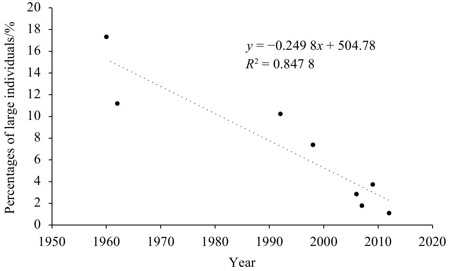
In this study, length frequencies of N. virgatus in the eight periods were analyzed at 10-mm standard length intervals. The dominant length groups were defined as the groups accounting for more than 10% of the total individuals and sex ratio as female-to-male ratio. Percentages of large individuals over time were analyzed by linear regression. We defined “large individuals” as the individuals with standard length more than 200 mm. This cut-off length was on the basis of the price categories of N. virgatus in seafood market and the individuals with length more than 200 mm were always classified to the highest category.
We used Shapiro-Wilk and Kolmogorov-Smirnov tests to check whether the raw data were normally distributed. Results showed the length data series in all eight years were not normally distributed (p<0.05). Therefore, we used “powerTransform” function in R package “car” to transform the data to normal distributions. Levene test was used to check the homogeneity of variance before parametric tests. Multiple Chi-squared tests were performed on gender data for the eight years to evaluate whether gender structure was consistent over any two neighbor years, thereby determine whether the sex ratio differs by year or not. The differences in mean length among the eight sampling years were tested by one-way analysis of variance (ANOVA). A post-hoc was conducted following the ANOVA test, i.e., differences in mean length between two years were checked by t test.
2.3
Length–weight relationship and relative condition factor
The power relationship between length and weight is described by the following equation:
$$ W = a{L^b}, $$
(1)
where W is wet weight (g) of an individual fish, L is standard length (mm), a is a condition factor, and b is an allometric growth parameter. Weight growth is isometric if b = 3, otherwise, weight growth is allometric (Nehemia et al., 2012). Differences between allometric factors b and 3 in the length–weight relationships were determined using paired-samples t tests.
The relative condition factor Wr compensates for changes in form or condition with increasing length, and thus measures the deviation of an individual from average weight for length (Le Cren, 1951). It compares the observed weight of an individual with the mean weight for that length:
$$ {W_{\rm{r}}} = \frac{W}{{a{L^b}}}. $$
(2)
A relative condition factor greater than one means the fish weighs more than expected for its length; a relative condition factor less than one means the fish weighs less than expected for its length. Differences in the relative condition factor between males and females were tested by t test.
2.4
Growth, mortality, and exploitation ratio
To estimate the tendency for growth to vary over time, the von Bertalanffy growth function (von Bertalanffy, 1938) was fitted for each sampling year separately, with the standard length defined as follows:
where Lt is the length at age t, L∞ is the asymptotic length, K is the growth coefficient (per year), and t0 is the hypothetical age at length zero. The growth parameters L∞ and K were estimated using FiSAT II software (version 1.2.2) through the restructured length-frequency data at 10-mm intervals, a method based on electronic length-frequency analysis (Pauly and David, 1981). The value of t0 was estimated using the empirical equation (Pauly, 1979) as follows:
To compare growth parameters among different sampling periods and different studies, a growth performance index φ′ (Pauly and Munro, 1984) was calculated as follows:
Total mortality (Z) was estimated using the length-converted catch curves based on pooled length-frequency data (Pauly, 1983), defined as follows:
$$ \ln ({N_i}/\Delta {t_i}) = c + dt_i', $$
(6)
$$ Z = - d, $$
(7)
where Ni is the number of fish caught in a given length class i, ti′ is the relative age corresponding to length class i, $\Delta $ti is the time needed, and c and d are the intercept and slope of the linear equation, respectively.
Natural mortality (M) was computed following Pauly (1980), as follows:
where L∞ is measured in cm and K in a−1. T represents the mean annual sea surface temperature (SST) in the Beibu Gulf, at 25.85°C (1960), 25.28°C (1962), 25.94°C (1992), 27.21°C (1998), 26.93°C (2006), 25.89°C (2007), 25.98°C (2009), and 25.80°C (2012). SST in the eight years were measured in the surveys and calculated as the average for all sampling stations and four seasons.
Based on the relationship between Z and M, fishing mortality (F) was calculated as follows:
$$ F{\text{ = }}Z - M. $$
(9)
The exploitation ratio (E) was obtained using the following equation:
$$ E = F/Z .$$
(10)
2.5
Standard length and age at median sexual maturity
Standard length and age at median sexual maturity were calculated using the data of female individuals during spawning seasons (April–June) of N. virgatus (Qiu et al., 2008). This analysis was conducted for only four years (1960, 1998, 2006, and 2012) as there were not enough female individuals measured during spawning seasons for other years. Maturity stages were determined on the basis of ovary development. We removed each individual’s exoskeleton to expose their ovaries and then identified the maturity stage by visual inspection. Each specimen was assigned to one of six stages; Stages I–III were considered sexually immature, and Stages IV–VI were considered sexually mature (Li et al., 2011). The standard length and age at median sexual maturity (L50 and A50) are essential reference points in fishery assessment (Hilborn and Walters, 1992). Logistic-type models, which are considered to be the best simple models for fitting maturity at length or maturity at age data, were applied to estimate L50 and A50 (Chen and Paloheimo, 1994). The proposed model for L50 is
where λ represents the instantaneous rate of maturation, and G the maximum attainable proportion of mature individuals. Because all individuals reach maturity after attaining a specific standard length, G = 1. Li is a midpoint value of the standard length interval, and εi is an error term. The arcsine-square root (ASR) transformative percentage Pi of maturity is given by the following equation:
The results of L50, λ, and their 95% confidence intervals were calculated by nonlinear regression. The A50 value was computed using the inverse von Bertalanffy growth function (von Bertalanffy, 1938) as follows:
The results show that sex ratio, body size, and length composition of N. virgatus stock have changed since 1960. The pooled population ranged from 36 mm to 316 mm in length and the sex ratios ranged from 1.63 to 4.12 (Fig. 3; Table 1) during the period from 1960 to 2012. Percentages of large individuals (standard length >200 mm) of N. virgatus show a significant downtrend over the sampling years (Fig. 4, p<0.05).
Table
1.
Population structure of Nemipterus virgatus in the Beibu Gulf from 1960 to 2012
The results of Chi-square tests indicated that sex ratios significantly differed between every two neighbor sampling years, i.e., 1960 and 1962 (χ2=23.05, p<0.05), 1962 and 1992 (χ2=4.59, p<0.05), 1992 and 1998 (χ2=8.57, p<0.05), 1998 and 2006 (χ2=157.63, p<0.05), 2006 and 2007 (χ2=12.38, p<0.05), 2007 and 2009 (χ2=8.47, p<0.05), and 2009 and 2012 (χ2=50.29, p<0.05). The length compositions significantly differed between males and females in all sampling years (p<0.05), but not in 2006 (χ2=1.82, p=0.19), and 2007 (χ2=1.21, p=0.28). The length compositions significantly differed between every two neighbor sampling years, i.e., 1960 and 1962 (χ2=21.32, p<0.05), 1962 and 1992 (χ2=37.39, p<0.05), 1992 and 1998 (χ2=52.44, p<0.05), 1998 and 2006 (χ2=78.96, p<0.05), 2006 and 2007 (χ2=12.23, p<0.05), 2007 and 2009 (χ2=9.35, p<0.05), and 2009 and 2012 (χ2=18.72, p<0.05).
The results of one-way ANOVA also revealed significant differences in average standard lengths among the eight sampling years (F=132.574, p<0.05). The results of t test showed there were significant differences mean length between 1960 and 2012 (t=15.59, p<0.05), 1962 and 2012 (t=11.82, p<0.05), 1992 and 2012 (t=15.07, p<0.05), 1998 and 2012 (t=10.87, p<0.05), 2006 and 2012 (t=3.45, p<0.05), 2007 and 2012 (t=8.90, p<0.05), except for 2007 and 2012 (t=−0.94, p=0.35).
3.2
Length–weight relationship and relative condition factor
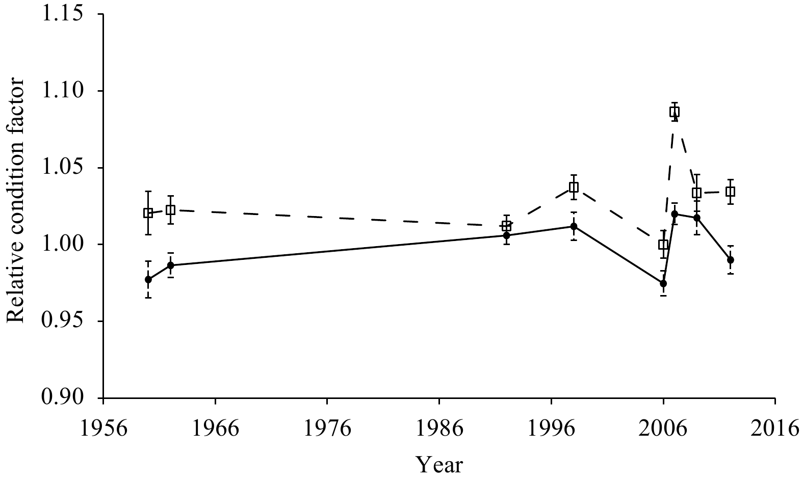
The condition factor and allometric growth parameter in the length–weight relationship varied over time for males and females (Table 2). During the period of 1960 to 2012, the condition factor of males ranged from 2.6×10⁻⁵ to 21.2×10⁻⁵ while that of females ranged from 3.2×10⁻⁵ to 25.7×10⁻⁵. The allometric growth parameter of males ranged from 2.56 to 2.98 while that of females ranged from 2.5 to 2.93. There were significant differences between the allometric growth parameter b and 3 (p<0.05) for males and females in the eight sampling years, except for males (t=1.47, p=0.19) and females (t=1.82, p=0.11) in 2006 and males (t=2.15, p=0.13) in 2007. The results of t tests revealed significant differences in the relative condition factor between males and females (p<0.05) in the eight sampling years, except for 1992 (t=1.91, p=0.19). Therefore, the relative condition factors of males were significantly lower than those of females, except in 1992 (Fig. 5). For both males and females, the highest relative condition factors were in 2007 and the lowest were in 2006.
Table
2.
Regression coefficient of length–weight relationship for male and female Nemipterus virgatus in the Beibu Gulf from 1960 to 2012
Year
Sex
df
a (×10−5)
95%CI (×10−5)
b
95%CI
R2
1960
male
186
11.1
5.2–23.8
2.68
2.53–2.82
0.96
female
253
7.9
5.6–11.1
2.73
2.67–2.80
0.98
1962
male
378
9.2
5.1–14.7
2.76
2.71–2.81
0.95
female
620
8.1
4.6–12.2
2.81
2.75–2.86
0.97
1992
male
138
7.9
5.5–11.0
2.78
2.73–2.82
0.98
female
212
7.4
4.8–10.3
2.82
2.78–2.87
0.98
1998
male
1107
8.6
7.12–10.3
2.74
2.70–2.78
0.95
female
1811
7.5
6.3–8.9
2.76
2.72–2.80
0.93
2006
male
184
2.6
1.9–3.4
2.98
2.92–3.03
0.98
female
765
3.2
2.7–3.8
2.93
2.89–2.97
0.97
2007
male
170
2.8
1.7–4.6
2.95
2.85–3.05
0.95
female
481
4.9
3.7–6.7
2.80
2.77–2.89
0.95
2009
male
151
5.7
3.0–10.9
2.80
2.67–2.93
0.92
female
614
24.5
17.8–33.7
2.50
2.43–2.56
0.90
2012
male
166
21.2
10.1–44.6
2.56
2.40–2.71
0.87
female
280
25.7
15.6–42.3
2.51
2.41–2.62
0.89
Note: CI represents confidence interval; df, freedom degree of linear regression.
Figure
5.
Temporal variation in relative condition factor of Nemipterus virgatus males (solid line) and females (dashed line) in the Beibu Gulf. Error bars indicate standard deviation.
The von Bertalanffy growth parameter for N. virgatus changed from 1960 to 2012 (Table 3). The asymptotic length L∞ had decreased to 312 mm in 2009 since the maximum (341 mm) in 1992. It was 320 mm in 2012, similar to that in 2006. The growth coefficient K ranged from 0.26 to 0.38 while the theoretical age at length zero ranged from –0.334 to –0.247 in the eight sampling years. The growth performance index φ′ varied between 2.44 and 2.63.
Table
3.
Estimated growth parameters of Nemipterus virgatus in the Beibu Gulf from 1960 to 2012
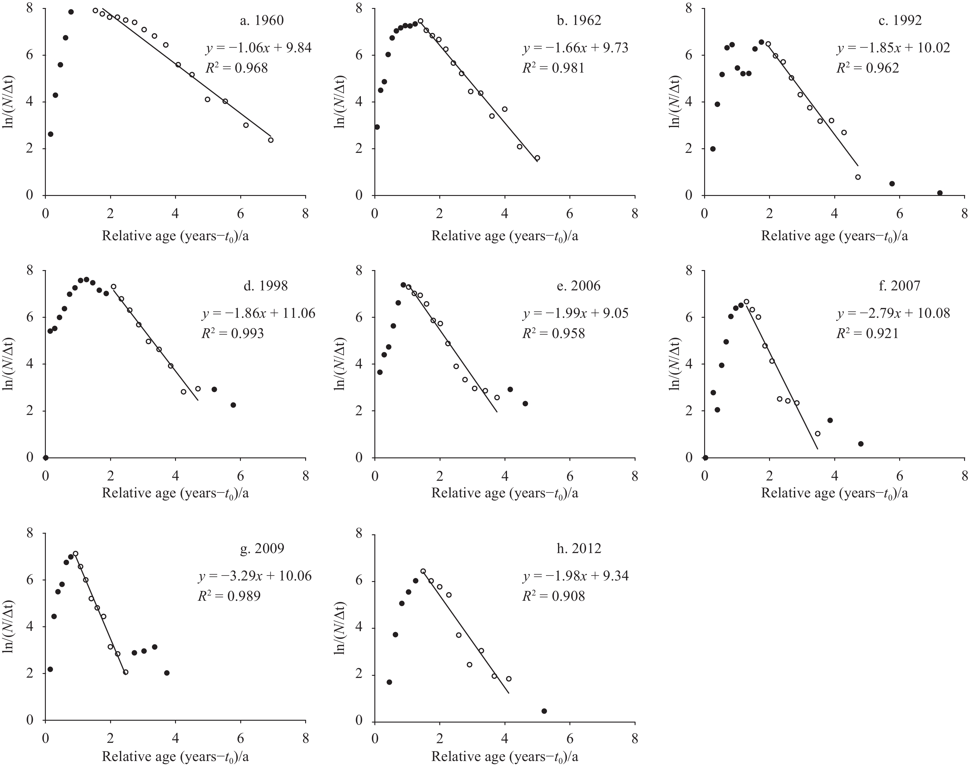
The total mortality coefficient Z was estimated from the length-converted catch curves (Fig. 6). The selection of regression data points was based on the principle that the age group without complete recruitment and the age group with a body length close to the asymptotic length could not be used for regression. All the p values of linear regressions in Fig. 6 were smaller than 0.05. The Z value first increased from 1.06 in 1960 to 3.29 in 2009, and then decreased to 1.98 in 2012 (Table 4). The natural mortality coefficient M varied between 0.70 and 0.88. The fishing mortality coefficient F increased from the lowest value (0.36) in 1960 to the highest value (2.43) in 2009, and then decreased in 2012 (1.10). The exploitation rate E was lower than 0.5 in 1960 and 1962, higher than 0.6 from 1992 to 2009, and 0.56 in 2012.
Figure
6.
Length-converted catch curves for Nemipterus virgatus in the Beibu Gulf from 1960 to 2012.
3.5
Standard length and age at median sexual maturity
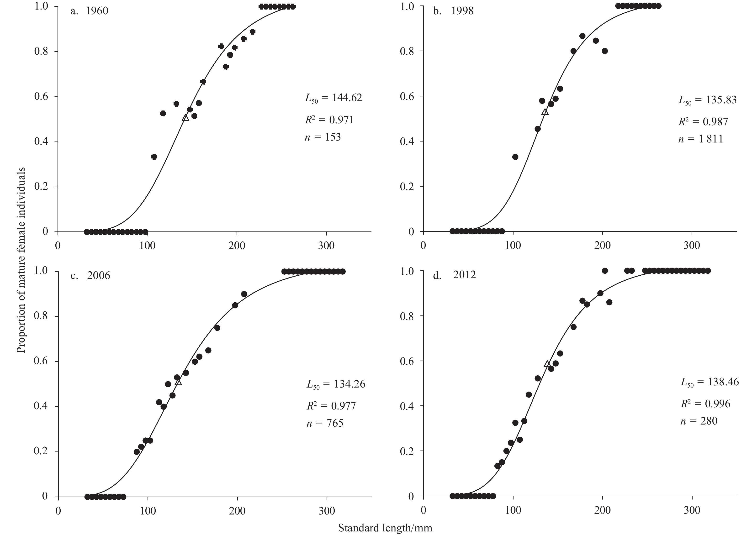
Based on an ASR logistic curve fitted by nonlinear regression (Fig. 7), the L50 values of N. virgatus were obtained. The L50 values were 144.62 mm (95% confidence interval (CI) 138.2–151.0 mm) in 1960, 135.83 mm (95%CI 131.5–140.2 mm) in 1998, 134.26 mm (95%CI 130.3–138.2 mm) in 2006, and 138.46 mm (95%CI 135.5–141.5 mm) in 2012. The corresponding A50 values calculated by the inverse von Bertalanffy growth function were 1.92 (95%CI 1.79–2.06), 1.65 (95%CI 1.57–1.74), 1.52 (95%CI 1.45–1.59) and 1.71 (95%CI 1.65–1.77), respectively.
Figure
7.
Proportion of mature female Nemipterus virgatus in the Beibu Gulf, and logistic curve fitted by ASR model. Dots represent observed data; triangles, L50.
Over the past six decades, significant variations in population structure, growth, mortality, sexual maturity, and exploitation rate of the N. virgatus stock in the Beibu Gulf have taken place. Average body length, estimated asymptotic length, dominant length groups and percentage of large individuals have decreased, indicating truncated size structure of a population. Estimated exploitation rates indicate that this stock was moderately exploited in 1960s and overexploited after 1992. This stock was taking a good turn in status in 2012, with the lowest exploitation rate since 1992 and ceased downward trend in length indexes.
4.1
Length–weight relationship
The length–weight relationship is a key factor in studies on the biology and management of fish species. This information is useful for predicting weight from length values, evaluating the condition of fish, and estimating biomass (Vaslet et al., 2008). It can also provide clues about environmental changes and sustainable management of fish stocks (Ecoutin et al., 2005). In this study, the value of the allometric growth parameter b was lower than 3 in most situations (Table 2), indicating negative allometric growth of N. virgatus in the Beibu Gulf. The relative condition factor Wr has been widely used in growth studies as it is an indicator of fish growth and the suitability of the environment. According to George et al. (1985), Wr indicates the general well-being of fish. Values of Wr higher than 1 are indicative of good well-being, while those lower than 1 reflect poor well-being of fish. In the present study, the Wr estimates of females were higher than 1 in the eight sampling years and generally higher than those of males (Fig. 5). This difference by sex was probably due to different energy allocation strategies adopted by males and females, and females might need to save more energy for spawning. The variation in the sex ratio over time may be another way of adjusting reproduction in different environments and life stages.
4.2
Shrinking of fish body size
Shrinking of fish body size is a common phenomenon among commercial fish species in marine and fresh waters worldwide (Sheridan and Bickford, 2011; Cheung et al., 2013), and especially in the four major sea areas of China. Since the 1960s, many important commercial fishes, such as small yellow croaker (Larimichthys polyactis) in the Bohai Sea and Yellow Sea (Li et al., 2011), largehead hairtail (Trichiurus lepturus) in the East China Sea (Zhou et al., 2002), and threadfin porgy (Evynnis cardinalis) in the SCS (Zhang et al., 2020a) have shown a reduction in body size alongside an increase in growth rate. There are three possible reasons for decreases in fish body size. The first is fishing-induced evolution (FIE). When size-selective fishing removes faster-growing individuals at higher rates than slower-growing fish, the surviving populations will become dominated by slower-growing individuals (Kraak et al., 2019). Therefore, the slower-growing fish genes have been inherited after long-term overfishing, as verified in populations of sockeye salmon (Oncorhynchus nerka) (Quinn et al., 2007) and Atlantic cod (Gadus morhua) (Olsen et al., 2004). The second explanation is the density-dependent effect. Overfishing creates a sparser population with diminishing predation and interspecific competition pressures, as well as sufficient food, allowing individuals with smaller body sizes to replenish the fishery (Kolluru and Reznick, 1996; Rouyer et al., 2011). The third explanation is the influence of climate change (Sinclair et al., 2002; Sheridan and Bickford, 2011). Li et al. (2011) studied the biological characteristics of L. polyactis in the Bohai Sea and Yellow Sea, and found that water temperature was closely related to the smaller body size and earlier sexual maturity. Both theory and empirical observations also support the hypothesis that warming and reduced oxygen will reduce body size of marine fish (Cheung et al., 2013). The Beibu Gulf is located in sub-tropical and tropical region, and variations in water temperature is smaller than northern seas. Overfishing has been occurred in main commercial fish species in the northern SCS since 1980s (Chen et al., 2011; Zhang et al., 2017). Therefore, overfishing seems to be the main driving force for shrinking of fish body size in the Beibu Gulf. As for it is FIE or density-dependent effect, further studies on changes in fish genes need to be done.
4.3
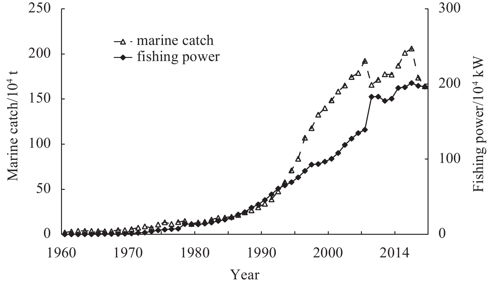
Exploitation status
As reported by Gulland (1983), the optimal utilization rate for fish is 0.5. Based on this suggested value, the N. virgatus resource in the Beibu Gulf was moderately exploited in 1960 and 1962 and overexploited after 1992. Since the 1950s, the catch in coastal waters has amounted to more than 90% of the total marine catch in China (Shan et al., 2016). The marine catches and total fishing power of Guangxi and Hainan (adjacent to the Beibu Gulf) have increased rapidly since the 1980s (Fig. 8). The total fishing power reached 195.0×10⁴ kW in 2018, while marine catches have fluctuated, with an average of 178×104 t over the last 15 a. Excessive fishing and a lack of effective management in recent decades has resulted in declining catch rates of commercial fish species (Qiu et al., 2008), shifts in fish community structure (Zhang et al., 2020b), and the collapse of fishery ecosystems (Chen et al., 2011) in typical semi-closed bays of the SCS. Five surveys conducted by the South China Sea Fisheries Research Institute from 1961 to 1999 revealed that the catch rates of N. virgatus in the Beibu Gulf had decreased from 16.4 kg/km2 in 1962 to 5.9 kg/km2 in 1998 (Wang and Yuan, 2008).
The main purpose for the management measures in recent decades were to halt the decline in fishery resources and conserve marine ecosystems. “Zero growth” and “Negative growth” policies could be considered as a kind of total allowable catch (TAC) controls (Shen and Heino, 2014), and claimed that the domestic marine catch should be equal to or lower than that of the previous year’s catch. The summer fishing moratorium was implemented to ensure that most species have a chance to spawn. It extended for 2 months initially, but was prolonged to 3.5 months in 2017 (Fig. 1). The “Double Control” system has been implemented to control the total number engine-powered fishing vessels and their total engine power. However, these strategies have not had a good overall effect (Shen and Heino, 2014). Meanwhile, other measures such as minimum mesh size regulation, the establishment of artificial reefs, fishery resource enhancement, and aquatic germplasm resource protection areas have been implemented to conserve fishery resources (Cao et al., 2017; Shen and Heino, 2014).
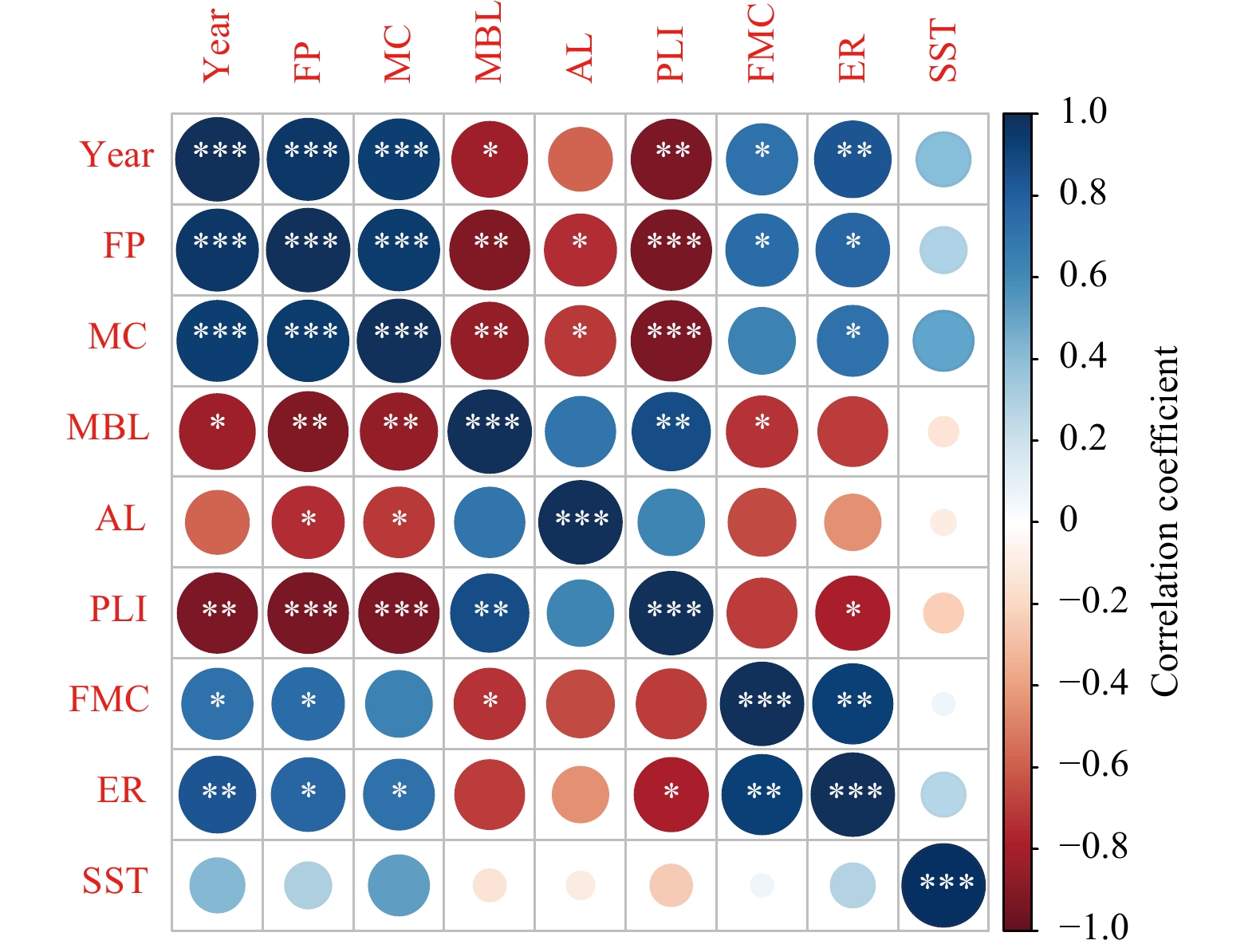
Correlations between biological characteristics and metrics of fishing pressure (Fig. 9) indicate that fishing pressure is the main cause of the reduction in the number of large individuals and shrinking body sizes of N. virgatus in the Beibu Gulf. The exploitation rate in 2012 was the lowest since 1992 (Table 4), and the downward trends in length indexes including mean body length (Table 2), asymptotic length (Table 3), and standard length at median sexual maturity (Fig. 6) also ceased in 2012. The results are similar to those reported for E. cardinalis, which showed increasing length indexes from 2006 to 2015 (Zhang et al., 2020a). Heavy exploitation of fish stocks can induce responses in phenotypic traits (Conover and Munch, 2002; Kuparinen and Merilä, 2007), as reported for haddock (Melanogrammus aeglefinus) and whiting (Merlangius merlangus) in the Firth of Clyde (Hunter et al., 2015). Therefore, management measures that aim to reduce fishing pressure may affect biological characteristics, given that variations in phenotypic traits seem reversible. The phenotypic plasticity of commercial fish species can reduce the economic value of the catch and fishing yield (Eikeset et al., 2013), and destabilize marine ecosystems (Pinsky and Palumbi, 2014). These findings highlight the importance of understanding the phenotypic plasticity of specific species like N. virgatus in fishery management.
Figure
9.
Correlation matrix for year, sea surface temperature (SST), mean body length (MBL), asymptotic length (AL), percentage of large individuals (PLI, standard length >200 mm), fishing mortality coefficient (FMC), and exploitation rate (ER) of Nemipterus virgatus in the Beibu Gulf, and fishing power (FP) and marine catches (MC) in Guangxi and Hainan, China; *, ** and *** represent the significance of the correlation p<0.05, p<0.01 and p<0.001, respectively.
We thank all those involved in the marine surveys that collected the data used in this study. We appreciate the valuable comments made by anonymous reviewers, which significantly improved our manuscript. We thank Jennifer Smith, from Liwen, Edanz Group China, for editing the English text of this manuscript.
Cao Ling, Chen Yong, Dong Shuanglin, et al. 2017. Opportunity for marine fisheries reform in China. Proceedings of the National Academy of Sciences of the United States of America, 114(3): 435–442. doi: 10.1073/pnas.1616583114
[2]
Chen Guobao, Li Yongzhen, Zhao Xianyong, et al. 2006. Acoustic assessment of five groups commercial fish in South China Sea. Haiyang Xuebao (in Chinese), 28(2): 128–134
[3]
Chen Yong, Paloheimo J E. 1994. Estimating fish length and age at 50% maturity using a logistic type model. Aquatic Sciences, 56(3): 206–219. doi: 10.1007/BF00879965
[4]
Chen Zuozhi, Qiu Yongsong, Xu Shannan. 2011. Changes in trophic flows and ecosystem properties of the Beibu Gulf ecosystem before and after the collapse of fish stocks. Ocean & Coastal Management, 54(8): 601–611
[5]
Chen Zuozhi, Xu Shannan, Qiu Yongsong, et al. 2009. Modeling the effects of fishery management and marine protected areas on the Beibu Gulf using spatial ecosystem simulation. Fisheries Research, 100(3): 222–229. doi: 10.1016/j.fishres.2009.08.001
[6]
Cheung W W L, Sarmiento J L, Dunne J, et al. 2013. Shrinking of fishes exacerbates impacts of global ocean changes on marine ecosystems. Nature Climate Change, 3(3): 254–258. doi: 10.1038/nclimate1691
[7]
Conover D O, Munch S B. 2002. Sustaining fisheries yields over evolutionary time scales. Science, 297(5578): 94–96. doi: 10.1126/science.1074085
[8]
Costello C, Ovando D, Hilborn R, et al. 2012. Status and solutions for the world’s unassessed fisheries. Science, 338(6106): 517–520. doi: 10.1126/science.1223389
[9]
Ecoutin J M, Albaret J J, Trap S. 2005. Length–weight relationships for fish populations of a relatively undisturbed tropical estuary: the Gambia. Fisheries Research, 72(2–3): 347–351
[10]
Eikeset A M, Richter A, Dunlop E S, et al. 2013. Economic repercussions of fisheries-induced evolution. Proceedings of the National Academy of Sciences of the United States of America, 110(30): 12259–12264. doi: 10.1073/pnas.1212593110
[11]
Fisheries Bureau of Ministry of Agriculture and Rural Affairs of China. 2019. China Fishery Statistics Yearbook (1960−2018). Beijing: China Agriculture Press, 38−84.
[12]
Froese R. 2004. Keep it simple: three indicators to deal with overfishing. Fish and Fisheries, 5(1): 86–91. doi: 10.1111/j.1467-2979.2004.00144.x
[13]
George J P, Sharma A K, Venkateshvaran K, et al. 1985. Length-weight relationship and relative condition factor in Cirrhinus mrigala and Labeo rohita from a sewage fed tank. The Annals of Zoology, 23: 70–90
[14]
Gulland J A. 1983. Fish Stock Assessment: A Manual of Basic Methods. New York: Wiley
[15]
Hilborn R, Walters C J. 1992. Quantitative Fisheries Stock Assessment: Choice, Dynamics and Uncertainty. New York, USA: Chapman & Hall
[16]
Hunter A, Speirs D C, Heath M R. 2015. Fishery-induced changes to age and length dependent maturation schedules of three demersal fish species in the Firth of Clyde. Fisheries Research, 170: 14–23. doi: 10.1016/j.fishres.2015.05.004
[17]
Khanh N O, Phu T D, Luong N T, et al. 2013. Appropriate fishing depths for squid longline fishery in the Gulf of Tonkin, Vietnam. Fish for the People, 11: 29–32
[18]
Kolluru G R, Reznick D N. 1996. Genetic and social control of male maturation in Phallichthys quadripunctatus (Pisces: Poeciliidae). Journal of Evolutionary Biology, 9(6): 695–715. doi: 10.1046/j.1420-9101.1996.9060695.x
[19]
Kraak S B M, Haase S, Minto C, et al. 2019. The Rosa Lee phenomenon and its consequences for fisheries advice on changes in fishing mortality or gear selectivity. ICES Journal of Marine Science, 76(7): 2179–2192. doi: 10.1093/icesjms/fsz107
[20]
Kuparinen A, Merilä J. 2007. Detecting and managing fisheries-induced evolution. Trends in Ecology & Evolution, 22(12): 652–659
[21]
Le Cren E D. 1951. The length-weight relationship and seasonal cycle in gonad weight and condition in the perch (Perca fluviatilis). Journal of Animal Ecology, 20(2): 201–219. doi: 10.2307/1540
[22]
Li Zhonglu, Shan Xiujuan, Jin Xianshi, et al. 2011. Long–term variations in body length and age at maturity of the small yellow croaker (Larimichthys polyactis Bleeker, 1877) in the Bohai Sea and the Yellow Sea, China. Fisheries Research, 110(1): 67–74. doi: 10.1016/j.fishres.2011.03.013
[23]
Nehemia A, Maganira J D, Rumisha C. 2012. Length–weight relationship and condition factor of tilapia species grown in marine and fresh water ponds. Agriculture and Biology Journal of North America, 3(3): 117–124. doi: 10.5251/abjna.2012.3.3.117.124
[24]
Olsen E M, Heino M, Lilly G R, et al. 2004. Maturation trends indicative of rapid evolution preceded the collapse of northern cod. Nature, 428(6986): 932–935. doi: 10.1038/nature02430
[25]
Palomares M L D, Pauly D. 2019. Coastal fisheries: the past, present, and possible futures. In: Wolanski E, Day J W, Elliott M, eds. Coasts and Estuaries: The Future. London, UK: Elsevier
[26]
Pauly D. 1979. Gill size and temperature as governing factors in fish growth: a generalization of von Bertalanffy’s growth formula. Berichte aus dem Institut fur Meereskunde an der Christian-Albrechts-Universitä t Kiel, 63: 156
[27]
Pauly D. 1980. On the interrelationships between natural mortality, growth parameters, and mean environmental temperature in 175 fish stocks. ICES Journal of Marine Science, 39(2): 175–192. doi: 10.1093/icesjms/39.2.175
[28]
Pauly D. 1983. Some Simple Methods for the Assessment of Tropical Fish Stocks. Rome, Italy: FAO Fisheries Department
[29]
Pauly D, David N. 1981. ELEFAN I, a BASIC program for the objective extraction of growth parameters from length-frequency data. Berichte der Deutschen Wissenschaftlichen Kommission für Meeresforschun, 28(4): 205–211
[30]
Pauly D, Munro J L. 1984. Once more on the comparison of growth in fish and invertebrates. ICLARM Fishbyte, 2: 21
[31]
Pauly D, Watson R, Alder J. 2005. Global trends in world fisheries: impacts on marine ecosystems and food security. Philosophical Transactions of the Royal Society B: Biological Sciences, 360(1453): 5–12. doi: 10.1098/rstb.2004.1574
[32]
Pauly D, Zeller D. 2016. Catch reconstructions reveal that global marine fisheries catches are higher than reported and declining. Nature Communications, 7: 10244. doi: 10.1038/ncomms10244
[33]
Pinsky M L, Palumbi S R. 2014. Meta-analysis reveals lower genetic diversity in overfished populations. Molecular Ecology, 23(1): 29–39. doi: 10.1111/mec.12509
[34]
Qiu Yongsong, Lin Zhaojin, Wang Yuezhong. 2010. Responses of fish production to fishing and climate variability in the northern South China Sea. Progress in Oceanography, 85(3–4): 197–212
[35]
Qiu Yongsong, Zeng Xiaoguang, Chen Tao, et al. 2008. Fishery Resources and Management in South China Sea (in Chinese). Beijing: China Ocean Press
[36]
Quinn T P, Hodgson S, Flynn L, et al. 2007. Directional selection by fisheries and the timing of sockeye salmon (Oncorhynchus nerka) migrations. Ecological Applications, 17(3): 731–739. doi: 10.1890/06-0771
[37]
Rouyer T, Ottersen G, Durant J M, et al. 2011. Shifting dynamic forces in fish stock fluctuations triggered by age truncation?. Global Change Biology, 17(10): 3046–3057
[38]
Russell B C. 1990. FAO Species Catalogue. Vol. 12. Nemipterid Fishes of the World. (Threadfin Breams, Whiptail Breams, Monocle Breams, Dwarf Monocle Breams, and Coral Breams). Family Nemipteridae. An Annotated and Illustrated Catalogue of Nemipterid Species Known to Date. Rome, Italy: FAO Fisheries Department
[39]
Shan Xiujuan, Jin Xianshi, Dai Fangqun, et al. 2016. Population dynamics of fish species in a marine ecosystem: a case study in the Bohai Sea, China. Marine and Coastal Fisheries, 8(1): 100–117. doi: 10.1080/19425120.2015.1114543
[40]
Shen Gongming, Heino M. 2014. An overview of marine fisheries management in China. Marine Policy, 44: 265–272. doi: 10.1016/j.marpol.2013.09.012
[41]
Sheridan J A, Bickford D. 2011. Shrinking body size as an ecological response to climate change. Nature Climate Change, 1(8): 401–406. doi: 10.1038/nclimate1259
[42]
Sinclair A F, Swain D P, Hanson J M. 2002. Disentangling the effects of size-selective mortality, density, and temperature on length-at-age. Canadian Journal of Fisheries and Aquatic Sciences, 59(2): 372–382. doi: 10.1139/f02-014
[43]
Turrero P, García-Vázquez E, de Leaniz C G. 2014. Shrinking fish: comparisons of prehistoric and contemporary salmonids indicate decreasing size at age across millennia. Royal Society Open Science, 1(2): 140026. doi: 10.1098/rsos.140026
[44]
Vaslet A, Bouchon-Navaro Y, Louis M, et al. 2008. Weight–length relationships for 20 fish species collected in the mangroves of Guadeloupe (Lesser Antilles). Journal of Applied Ichthyology, 24(1): 99–100
[45]
von Bertalanffy L. 1938. A quantitative theory of organic growth (inquiries on growth laws II). Human Biology, 10(2): 181–213
[46]
Wang Xuehui, Qiu Yongsong, Du Feiyan. 2004. Study on the growth, mortality and optimum catchable size of Nemipterus virgatus in the northern South China Sea. Journal of Ocean University of China, 34(2): 224–230
[47]
Wang Yuezhong, Yuan Weiwen. 2008. Changes of demersal trawl fishery resources in northern South China Sea as revealed by demersal trawling. South China Fisheries Science, 4(2): 26–33
[48]
Zhang Kui, Cai Yancong, Liao Baochao, et al. 2020a. Population dynamics of threadfin porgy Evynnis cardinalis, an endangered species on the IUCN red list in the Beibu Gulf, South China Sea. Journal of Fish Biology, 97(2): 479–489. doi: 10.1111/jfb.14398
[49]
Zhang Kui, Guo Jianzhong, Xu Youwei, et al. 2020b. Long-term variations in fish community structure under multiple stressors in a semi-closed marine ecosystem in the South China Sea. Science of the Total Environment, 745: 140892. doi: 10.1016/j.scitotenv.2020.140892
[50]
Zhang Kui, Liao Baochao, Xu Youwei, et al. 2017. Assessment for allowable catch of fishery resources in the South China Sea based on statistical data. Haiyang Xuebao (in Chinese), 39(8): 25–33
[51]
Zhou Yongdong, Xu Hanxiang, Liu Zifan, et al. 2002. A study on variation of stock structure of Hairtail (Trichiurus haumela) in the East China Sea. Journal of Zhejiang Ocean University: Natural Science, 21: 314–320
Jinrun Wang, Haiyan Zhang, Chuanhao Pan, et al. Spatial and temporal patterns in Pelagic Fish Egg Assemblages in Spring and Late Autumn–winter in Eastern Beibu Gulf. Marine Environmental Research, 2025. doi:10.1016/j.marenvres.2025.107066
2.
Hagai Nsobi Lauden, Shaoliang Lyu, Alma Alfatat, et al. Population dynamics and seasonal variation in biological characteristics of black sea bream (Acanthopagrus schlegelii) in Zhanjiang coastal waters, China. Frontiers in Marine Science, 2025, 11 doi:10.3389/fmars.2024.1515753
3.
Li Su, Kui Zhang, Youwei Xu, et al. Variations in the fish community of the Beibu Gulf (South China Sea) following fishery resources protection measures. Fisheries Research, 2025, 283: 107293. doi:10.1016/j.fishres.2025.107293
4.
Xiaofan Hong, Kui Zhang, Jiajun Li, et al. Stock Assessment of the Commercial Small Pelagic Fishes in the Beibu Gulf, the South China Sea, 2006–2020. Biology, 2024, 13(4): 226. doi:10.3390/biology13040226
5.
Hagai Nsobi Lauden, Xinwen Xu, Shaoliang Lyu, et al. Assessment of the Fish Stock Status Using LBSPR with Its Implications on Fisheries Management: A Case Study of Nemipterus virgatus, Priacanthus macracanthus, and Saurida undosquamis in the Northern South China Sea. Journal of Applied Ichthyology, 2024, 2024(1) doi:10.1155/2024/6808795
6.
Hagai Nsobi Lauden, Xinwen Xu, Shaoliang Lyu, et al. Fish Stock Status and Its Clues on Stocking: A Case Study of Acanthopagrus schlegelii from Zhanjiang Coastal Waters, China. Fishes, 2024, 9(10): 381. doi:10.3390/fishes9100381
7.
Jiajun Li, Zhixin Zhang, Kui Zhang, et al. Tracking the Development of Lit Fisheries by Using DMSP/OLS Data in the Open South China Sea. Remote Sensing, 2024, 16(19): 3678. doi:10.3390/rs16193678
8.
Youwei Xu, Peng Zhang, Sher Khan Panhwar, et al. The initial assessment of an important pelagic fish, Mackerel Scad, in the South China Sea using data-poor length-based methods. Marine and Coastal Fisheries, 2023, 15(5) doi:10.1002/mcf2.10258
9.
Lei Xu, Feiyan Du, Quehui Tang, et al. Seasonal variability of nektonic community structure and phylogenetic diversity in Weizhou Island, the Beibu Gulf. Frontiers in Marine Science, 2023, 10 doi:10.3389/fmars.2023.1133462
10.
Youwei Xu, Kui Zhang, Mingshuai Sun, et al. Tempo-Spatial Distribution of an Endangered Fish Species, Threadfin Porgy Evynnis cardinalis (Lacepède, 1802), in the Northern South China Sea. Journal of Marine Science and Engineering, 2022, 10(9): 1191. doi:10.3390/jmse10091191
11.
Qi Ding, Xiujuan Shan, Xianshi Jin, et al. Achieving greater equity in allocation of catch shares: A case study in China. Frontiers in Marine Science, 2022, 9 doi:10.3389/fmars.2022.1049893
12.
Kui Zhang, Miao Li, Jiajun Li, et al. Climate-induced small pelagic fish blooms in an overexploited marine ecosystem of the South China Sea. Ecological Indicators, 2022, 145: 109598. doi:10.1016/j.ecolind.2022.109598
Kui Zhang, Ping Geng, Jiajun Li, Youwei Xu, Muhsan Ali Kalhoro, Mingshuai Sun, Dengfu Shi, Zuozhi Chen. Influences of fisheries management measures on biological characteristics of threadfin bream (Nemipterus virgatus) in the Beibu Gulf, South China Sea[J]. Acta Oceanologica Sinica, 2022, 41(3): 24-33. doi: 10.1007/s13131-021-1925-9
Kui Zhang, Ping Geng, Jiajun Li, Youwei Xu, Muhsan Ali Kalhoro, Mingshuai Sun, Dengfu Shi, Zuozhi Chen. Influences of fisheries management measures on biological characteristics of threadfin bream (Nemipterus virgatus) in the Beibu Gulf, South China Sea[J]. Acta Oceanologica Sinica, 2022, 41(3): 24-33. doi: 10.1007/s13131-021-1925-9
Figure 1. Marine fishery catches in the South China Sea and timeline of the introduction of management measures and policy priorities. Most of the measures were synchronous with other seas in China, except for the summer fishing moratorium.
Figure 2. Map of the Beibu Gulf and sampling stations.
Figure 3. Length frequency distributions of Nemipterus virgatus in the Beibu Gulf from 1960 to 2012.
Figure 4. Percentage of large individuals (standard length>200 mm) of Nemipterus virgatus in the Beibu Gulf in different sampling years.
Figure 5. Temporal variation in relative condition factor of Nemipterus virgatus males (solid line) and females (dashed line) in the Beibu Gulf. Error bars indicate standard deviation.
Figure 6. Length-converted catch curves for Nemipterus virgatus in the Beibu Gulf from 1960 to 2012.
Figure 7. Proportion of mature female Nemipterus virgatus in the Beibu Gulf, and logistic curve fitted by ASR model. Dots represent observed data; triangles, L50.
Figure 9. Correlation matrix for year, sea surface temperature (SST), mean body length (MBL), asymptotic length (AL), percentage of large individuals (PLI, standard length >200 mm), fishing mortality coefficient (FMC), and exploitation rate (ER) of Nemipterus virgatus in the Beibu Gulf, and fishing power (FP) and marine catches (MC) in Guangxi and Hainan, China; *, ** and *** represent the significance of the correlation p<0.05, p<0.01 and p<0.001, respectively.


 DownLoad:


 DownLoad:


 DownLoad:


