

Figure
1.
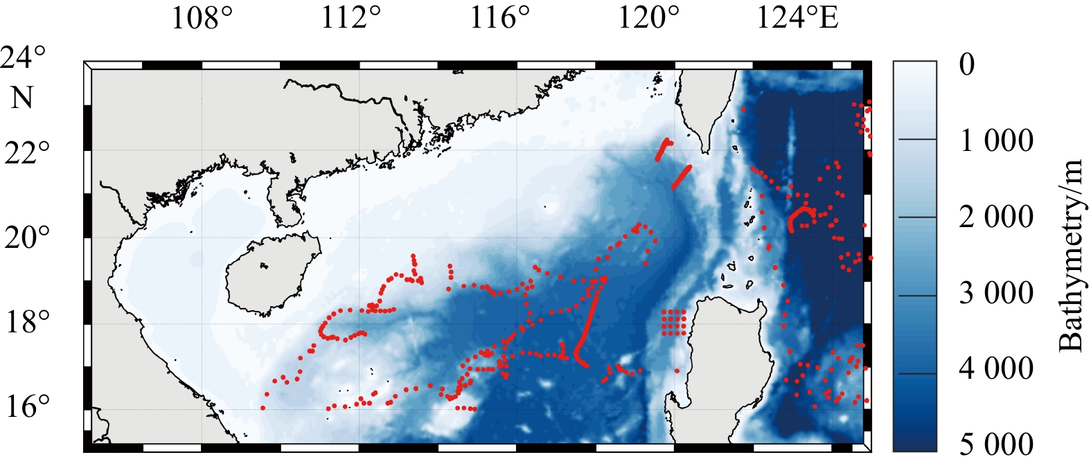
Model domain and bathymetry in the northern South China Sea. The red points are the locations of the T/S profiles.
| Citation: | Meng Shen, Yan Chen, Pinqiang Wang, Weimin Zhang. Assimilating satellite SST/SSH and in-situ T/S profiles with the Localized Weighted Ensemble Kalman Filter[J]. Acta Oceanologica Sinica, 2022, 41(2): 26-40. doi: 10.1007/s13131-021-1903-2

|
Data assimilation (DA) is playing an increasingly important role in the numerical prediction of atmosphere and ocean. It can improve the analysis and prediction effects of a model by continuously integrating observations (Shen et al., 2016) and can also be used to optimize parameters of the model.
The most widely used ocean DA methods are variational methods and the ensemble Kalman filter (EnKF). The four-dimensional variational (4D-Var) method is a variational method that obtains the best trajectory by minimizing the cost function. Compared with 4D-Var, the EnKF does not need to construct the tangent linear or adjoint operators of the model and can estimate the background error covariance matrix using an ensemble. The limitations of the EnKF lie in the implicit assumption of model linearity in the background error covariance matrix calculation and Gaussian distributions of model error and observation error. Thus, in theory, the EnKF may not be applicable to strong nonlinear/non-Gaussian systems. In earlier studies, oceanographers assumed that changes in the ocean occurred slowly and thus that the evolution of the ocean involved a weakly nonlinear process. However, mesoscale eddies have strong nonlinear characteristics (Zhang et al., 2020). To better characterize nonlinear evolution in the ocean, nonlinear DA methods such as the particle filter (PF) have received increasing attention.
Both the PF and EnKF are based on the statistical estimation theory. Compared with the EnKF, the PF is not limited by the linear model, linear/weak nonlinear observations or the hypothesis of Gaussian-distributed error and can be applied to any nonlinear/non-Gaussian dynamic system in theory. In the PF, the probability density function (PDF) of states is approximated by the weighted mean of the particles. The observations affect the weights of the particles rather than the values of the particles. With assimilation progress, most particles cannot obtain meaningful weights (close to 0) due to the large gap between them and observations, which is known as filter degeneracy in the PF. To alleviate or overcome filter degeneracy, four main techniques were introduced to the PF, including proposal density, transportation, localization and hybridization (van Leeuwen et al. 2019).
The basic idea of localization is calculating particle weights locally. The PF localization techniques can be divided into two categories (Farchi and Bocquet, 2018). One is state-domain localization, which independently analyzes grid points using only the observations in a localized region. This approach is easy to implement in parallel but may lead to an imbalance between state variables. The related studies include Rebeschini and van Handel (2015), Penny and Miyoshi (2016), Lee and Majda (2016), and Chustagulprom et al. (2016). The other is sequential-observation localization. In this method, each observation is sequentially assimilated. An analysis is implemented at each observation site, and only the model variables near the observation site are updated. The local particle filter (LPF) proposed by Poterjoy (2016) (called the LPF16 hereafter) falls under this category.
LPF16 extends the scalar weight of the particle to a vector of the same dimension as the variables and changes only the weights of local model variables when assimilating each observation. Then, the variables near the observation are updated, and the prior information remains unchanged for the variables outside the localization radius. The weights of adjacent grid model variables in the LPF16 are obtained by spatial linear interpolation. Shen et al. (2017) introduced a new calculation formula for local weight, and the interpolation in the weight space was replaced by the calculation in the state space. The improved method has been tested only in the Lorenz 96 model and has not been applied to complex high-dimensional models. Poterjoy et al. (2019) made a series of improvements to the LPF16, including the weight formula calculation, observation error variance inflation, and the merger scheme. The improved method is called LPF19. The LPF19 has already been applied in numerical weather prediction systems (Poterjoy et al., 2019).
The idea of the proposal density technique is to sample particles from the proposal density introduced artificially instead of from the state transition density. The proposal density only needs to meet its support set, which contains the original state transition density. Theoretically, the proposal density can be constrained by both the model and observations so that the particles can be artificially close to the observed value to prevent the particle weights from becoming too low, thus effectively alleviating filter degeneracy. Proposal density provides a method for combining different technologies or approaches. Papadakis et al. (2010) proposed the Weighted Ensemble Kalman Filter (WEnKF), which takes the EnKF as the proposal density. The main goal is to take the posterior probability density obtained from the EnKF as the proposal density of the PF, calculate the weight, and obtain the posterior ensemble from the resampling scheme. van Leeuwen et al. (2015) point out that this method is not suitable for high-dimensional problems. However, taking the EnKF as the proposal density is a beneficial way for the development of the PF, and Sebastien et al. (2013) conducted relevant studies in this area. Wang et al. (2020) proposed the implicit equal-weights variational particle smoother (IEWVPS) based on the proposal density technique. The IEWVPS uses the 4D-Var as a proposal density to combine the PF with the 4D-Var and it has potential applications in higher dimensional model. Wang et al. (2021) have applied this method to Regional Ocean Modelling System (ROMS) with good results. It is computationally more expensive due to its use of 4D-Var as the proposed density.
Chen et al. (2020b) proposed Localized Weighted Ensemble Kalman Filter (LWEnKF) based on the WEnKF method combined with localization technology. Similar to the WEnKF, the stochastic EnKF is used as the proposal density in LWEnKF. In the calculation of particle weights in the LWEnKF, scalar weights are extended to vectors as in the LPF16, and only the model variables within the local radius are modified. In the LWEnKF framework, the particle weight is determined by the likelihood weight and proposal weight. The likelihood weight is constrained by observations, while the proposal weight is constrained by observations and the model. In Chen et al. (2020a), the LWEnKF was improved by introducing a localization technique to the proposal weight calculation and was applied to the high-dimensional ocean model ROMS, assimilating grided sea surface observations and T/S profiles. However, in terms of operational applications, real-time is very important. Thus, along-track observations instead of gridded data are more suitable for operational systems. It also should be noted that along-track observations are sparser than gridded data. The performance of the LWEnKF for sparse data assimilation still needs to be tested.
In this paper, the ability of the LWEnKF to assimilate along-track sea surface height (AT-SSH) is tested, swath sea surface temperature (S-SST) and in-situ temperature and salinity (T/S) profiles, as a reference for the operational application of the method. For objectivity, the results of the LWEnKF are compared with those of the EnKF and LPF19, the former is a classic method and suitable for the linear and weak nonlinear situation while the latter is a nonlinear method.
This paper is organized as follows. In Section 2, the assimilation system is introduced, including assimilation methods, ocean models and observations. In Section 3, the performance of different methods and the prediction ability of the LWEnKF assimilation system for mesoscale eddies are evaluated. The conclusions and discussion are presented in the last section.
The LWEnKF assimilation system is based on the Data Assimilation Research Testbed (DART) platform developed by the National Center for Atmospheric Research (NCAR). DART integrates multiple ensemble assimilation algorithms such as the EnKF and LPF19 and provides interfaces for large geophysical models such as the ROMS and the Massachusetts Institute of Technology ocean general circulation model (MITgcm).
The ROMS is implemented in the northern South China Sea (SCS), which is a region characterized by large scale wind-driven circulation and active mesoscale eddies and which is suitable for the study of nonlinear data assimilation. Figure 1 shows the model domain which spans from 15°N to 24°N and 105°E to 125°E with a horizontal resolution of (1/6)° × (1/6)° and 24 vertical levels. The bathymetry is ETOPO2 with
The observations used in the assimilation experiments are AT-SSH, S-SST and T/S profiles. AT-SSH data are obtained from the Copernicus Marine Environment Monitoring Service (CMEMS) with a mean dynamic topography (MDT) from a seven-year (2007 to 2013) free run of the ROMS. S-SST data are obtained from a L2P data product of the Group for High Resolution Sea Surface Temperature (GHRSST). A super-observation scheme is adopted to assimilate S-SST. T/S profiles are obtained from EN4.2.1 observation data set (Good et al., 2013) published by the Met Office Hadley Centre. Although the T/S profiles are quality-controlled, there are still outliers. To remove outliers, the data are quality controlled further and interpolated to standard artificial layers. The data from EN4.2.1 are quality controlled and the details of the quality control process can be found in Ingleby and Huddleston (2007) and Good et al. (2013). The data with the quality control flags marked as “1” are applied to assimilation systems. Although the T/S profiles are quality-controlled, there are still outliers. For processing convenience, all the profiles are interpolated to the artificial layers (5 m, 10 m, 15 m, 20 m, 25 m, 30 m, 35 m, 40 m, 50 m, 60 m, 75 m, 100 m, 125 m, 150 m, 200 m, 250 m, 300 m, 400 m, 500 m, 600 m, 800 m, 1 000 m, 1 200 m) using spline interpolation. Then, observations were further examined using the standard deviation at each layer. Specifically, observations were removed if the absolute deviation to the horizontal mean value is greater than 1.5 times of the standard deviation at each layer. Last, a super observation was created to adapt the vertical coordinates of ROMS. This is necessary when more than one observation exists in a grid cell at the same time.
The verification data include gridded sea level anomaly (SLA) products from Archiving Validation and Interpretation of Satellite Oceanographic (AVISO), surface currents from ocean surface current analysis real-time (OSCAR; Bonjean and Lagerloef, 2002) and gridded SST products from the Advanced Very High Resolution Radiometer (AVHRR).
Anderson (2003) proposed a sequential localization scheme for the EnKF that can be carried out in two steps when processing a single observation. First, for each prior ensemble, the analysis increment of the observation space is obtained. Second, a linear regression is performed for each state variable on the observation variable near the observation position in the prior ensemble. The updated increment of the state space is obtained from the increments of the observation space. The state space increments are added to the prior states to obtain the final analysis state.
LPF16 also adopts a framework of sequential assimilation. In the LPF16, the scalar weight of the particle is extended to a vector, and each model variable has a corresponding weight, which means that the influence of an observation on the weight can be localized. For a single observation, the LPF16 updates the weights of the variables only near that observation. To prevent a false reduction in posterior sample variance after resampling, the local weight is multiplied by a scalar coefficient
The LWEnKF takes the perturbed EnKF as the proposal density, which is sampled to obtain the proposal particle and calculate the proposal weight, which is calculated using observations and local model variables. The proposal weight also needs to be adjusted by parameter
The local radius in the assimilation system is controlled by the local parameter
| $$ {C}_{0}\left(z,\dfrac{1}{2},l\right)=\left\{\begin{array}{*{20}{l}}-\dfrac{1}{4}{\left(\dfrac{z}{l}\right)}^{5}+\dfrac{1}{2}{\left(\dfrac{z}{l}\right)}^{4}+\dfrac{5}{8}{\left(\dfrac{z}{l}\right)}^{3}-\dfrac{5}{3}{\left(\dfrac{z}{l}\right)}^{2}+1,&0\leqslant \left|z\right|\leqslant l,\\ \dfrac{1}{12}{\left(\dfrac{z}{l}\right)}^{5}-\dfrac{1}{2}{\left(\dfrac{z}{l}\right)}^{4}+\dfrac{5}{8}{\left(\dfrac{z}{l}\right)}^{3}+\dfrac{5}{3}{\left(\dfrac{z}{l}\right)}^{2}-5\dfrac{z}{l}+4-\dfrac{2l}{3z},&l < \left|z\right| < 2l,\\ 0,&2l\leqslant \left|z\right|,\end{array}\right. $$ | (1) |
where
| $$ \left\{\begin{array}{c}{l}_{{\rm{h}}}=2c\cdot {R},\\ {l}_{{\rm{v}}}=2c\cdot L,\end{array}\right. $$ | (2) |
where
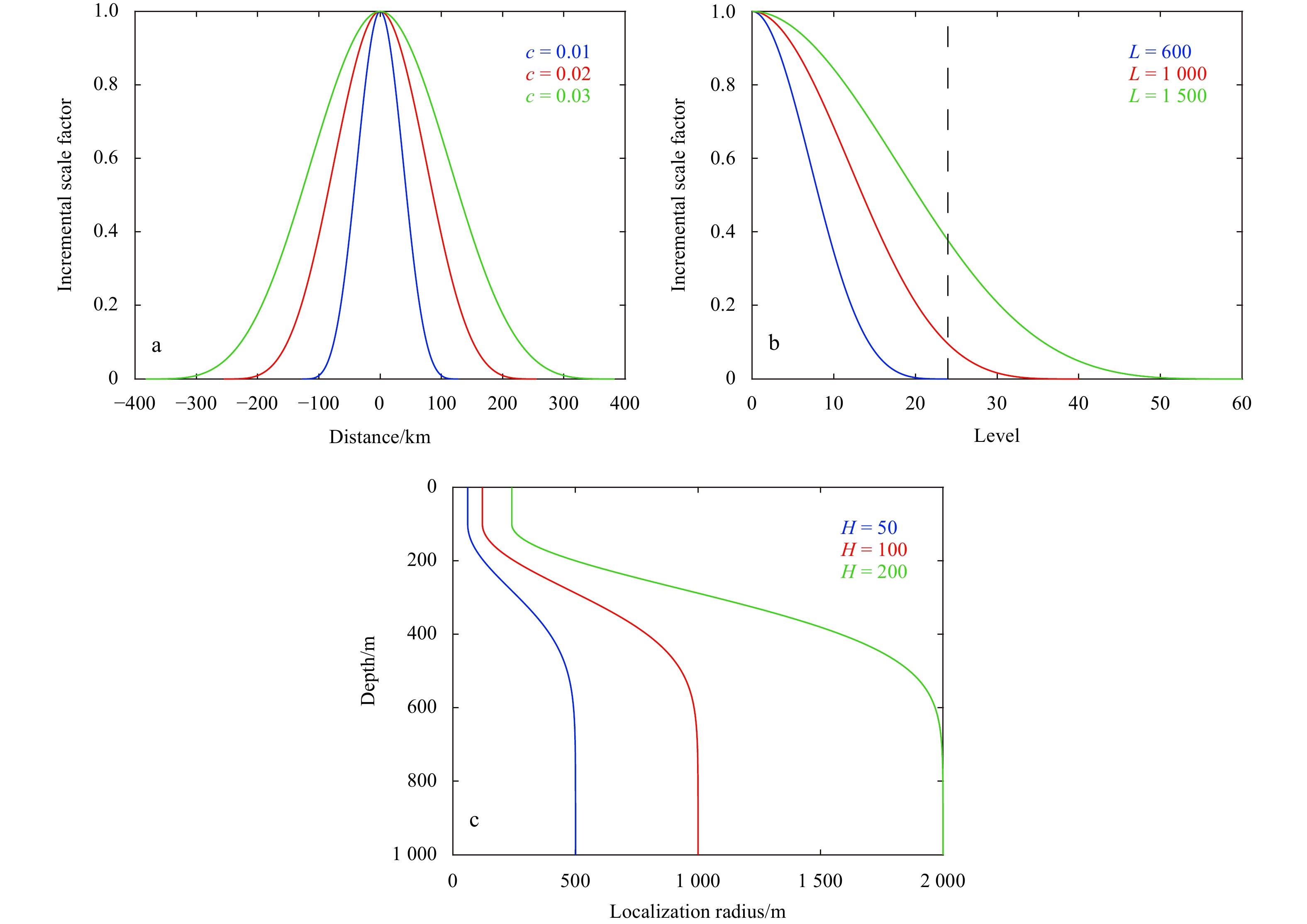
The vertical local radius function for T/S profiles is designed as Eq. (3). The functional design is adapted to the vertical S-coordinates of the ROMS, and the local radii corresponding to different observation depths are shown in Fig. 2c.
| $$ {l}'_{{\rm{v}}}=\left\{\begin{array}{*{20}{l}}2\cdot c\cdot H\cdot b,& h < -100,\\ 2\cdot c\cdot H\left\{a\cdot \left[1-\mathrm{exp}\left(-\dfrac{h-{h}_{1}}{{{h}_{2}}^{2}}\right)\right]+b\right\},& h\geqslant -100,\end{array}\right. $$ | (3) |
where
All experiments presented in this paper use 40 particles or ensembles. The optimal localization parameter
It is important for initial state ensembles to consider the main physical quantities that govern the evolution of the state of atmospheric and oceanic systems (Hoteit et al., 2008). A similar method to Hoteit et al. (2013) is adopted to generate the initial ensemble. First, integrate the model over a long period of time (2007–2014). Second, extract the dominant variability from the long model trajectory via empirical orthogonal function (EOF) analysis. Finally, generate the initial ensemble by an exact second-order sampling scheme (Pham, 2001):
| $$ x_0^i=x+\sqrt{N}{\boldsymbol{L}}_{0}{\text{σ}}_{i}^{\rm{T}} , $$ | (4) |
where x is the initial state of assimilation extracted from the long model trajectory;
To increase the spread of prior ensembles during assimilation, atmospheric forcing variables are perturbed following Chen et al. (2020a):
| $$ f_i={f}+0.2\sqrt{N}{\boldsymbol{L}}{{{\text{σ}}}}_{i}^{\rm{T}} , $$ | (5) |
where f are the perturbed variables, including surface wind stress and surface net heat flux. The generation of the perturbed variables is similar to the initial ensemble perturbation. EOF analysis is used to extract the main variability of the variables. The rest of the forcing variables are not perturbed.
Several questions are considered when designing the experiments. First, can the simultaneous assimilation of S-SST and AT-SSH outperform single surface observational variable assimilation? Second, is there different performance regarding different assimilation methods? If yes, what are the differences? Third, does the LWEnKF assimilation system have advantages in predicating mesoscale eddy?
The experimental design is shown in Table 1.
| Experiment | Method | Assimilated variables |
| ExpA | Control run | none |
| ExpB1 | LWEnKF | AT-SSH |
| ExpB2 | S-SST | |
| ExpB3 | AT-SSH, S-SST | |
| ExpC1 | EnKF | AT-SSH |
| ExpC2 | S-SST | |
| ExpC3 | AT-SSH, S-SST | |
| ExpD1 | LPF19 | AT-SSH |
| ExpD2 | S-SST | |
| ExpD3 | AT-SSH, S-SST | |
| ExpE1 | LWEnKF | AT-SSH, S-SST, T/S profiles |
| ExpE2 | EnKF | AT-SSH, S-SST, T/S profiles |
| ExpE3 | LPF19 | AT-SSH, S-SST, T/S profiles |
 DownLoad:
CSV
DownLoad:
CSV
In Table 1, ExpA is a control experiment without assimilation; ExpB, ExpC and ExpD assimilate only satellite observations; and ExpE adds additional T/S profiles. The assimilation experiments were conducted from October 3, 2013 to February 1, 2014, for a total of 120 days, which is identical to 30 assimilation cycles (four-day assimilation window). Within a window, observations within ±2 days of the analysis time are assimilated.
This section focuses on the discussion of the experimental results of ExpA−ExpD and explores whether simultaneous assimilation of S-SST and AT-SSH can achieve better results than single variable assimilation.
In Fig. 3, the dotted lines show the root mean square errors (RMSEs) of the three methods with only S-SST assimilation, solid lines denote the results with both AT-SSH and S-SST assimilation, and the black solid line shows the result of the control experiment. In the control experiment, the RMSE increased gradually with time without constraints from observations. Based on the RMSE trends, the three assimilation methods improved the observation variable SST, but the assimilation effect of the LPF19 is not ideal. The RMSE of the LPF19 shows the same trend as that of the control experiment, while the assimilation effect of the EnKF and LWEnKF is obvious. Compared to the control experiment, the EnKF and LWEnKF reduce the RMSE by 41.95% and 47.99% according to the forecast results (Fig. 3a) for assimilating S-SST alone, respectively. The four-day forecast in figures means the forecast results at the fourth forecast day. For the analysis results (Fig. 3b), the EnKF and LWEnKF reduce the average RMSE by 55.61% and 59.82%, respectively. When both S-SST and AT-SSH are assimilated, the forecast results (Fig. 3a) show that EnKF and LWEnKF reduce the average RMSE by 51.97% and 52.33%, respectively. For the analysis results (Fig. 3b), the EnKF and LWEnKF reduce the average RMSE by 61.15% and 61.73%, respectively. The readers should note that the percentages are calculated using the data before the two significant digits are retained, so the average RMSEs in the figure are equal and the calculated percentages are slightly different. For both AT-SSH and S-SST assimilation, the EnKF and LWEnKF show better assimilation effects than for S-SST assimilation alone based on the RMSE time series and the statistical average RMSE results. This result indicates that AT-SSH assimilation has a positive effect on the simulation of SST. The LWEnKF is comparable with the EnKF for S-SST assimilation alone. In the case of both AT-SSH and S-SST assimilation, the LWEnKF is no worse than the EnKF.
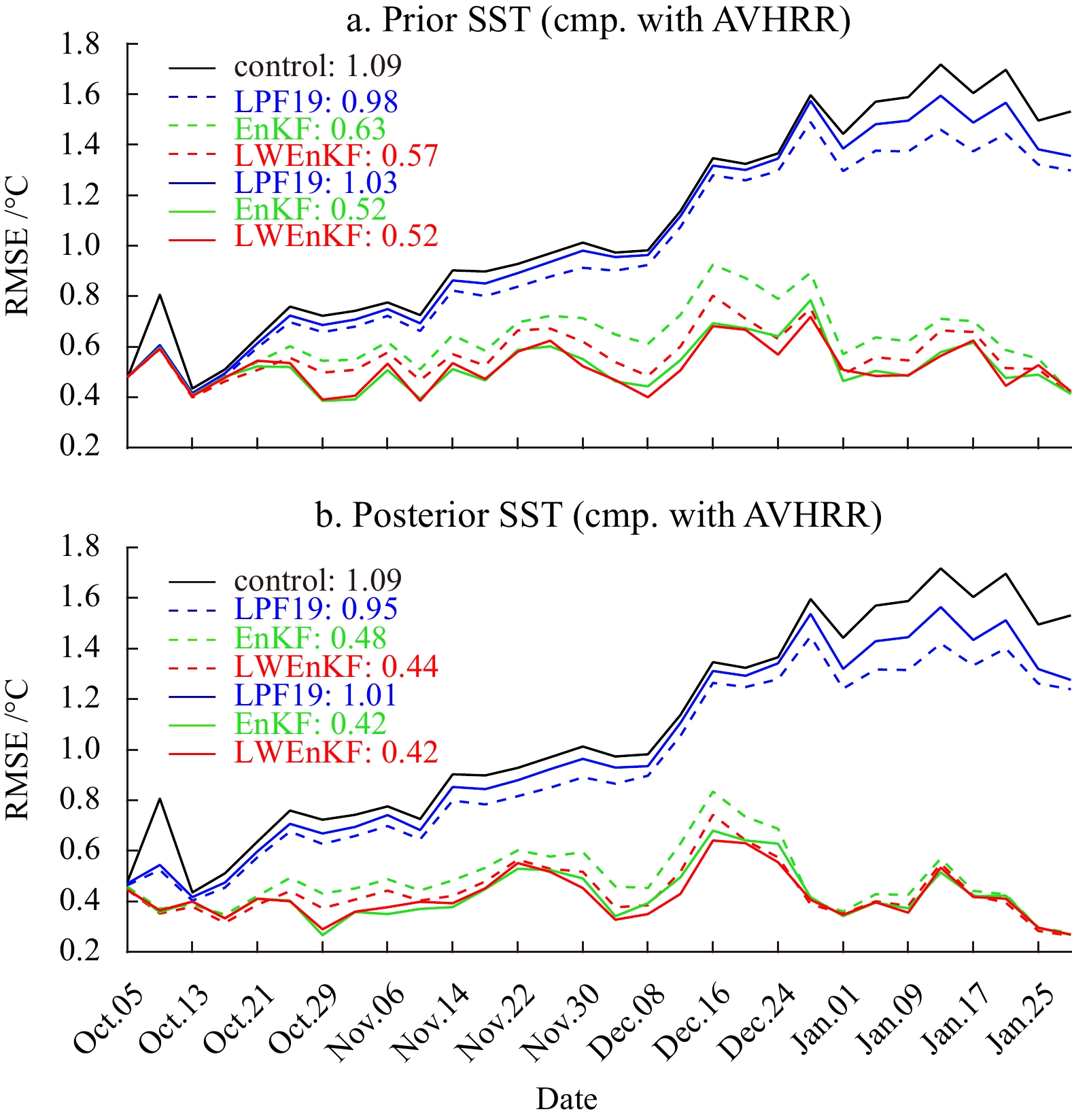
In Fig. 4, the dotted lines show the RMSEs of the three methods with only AT-SSH assimilation, the solid lines are the results with both AT-SSH and S-SST assimilation, and the black solid line shows the result of the control experiment. The trends of the RMSEs of the three methods are basically the same, and RMSEs fluctuate greatly at the beginning and tend to be stable in the later stage. Compared to the control experiment, the EnKF and LWEnKF reduce the RMSE by 36.60% and 30.58% according to the forecast results (Fig. 4a) for assimilating AT-SSH alone, respectively. For the analysis results (Fig. 4b), the EnKF and LWEnKF reduce the average RMSE by 50.47% and 44.29%, respectively. When both S-SST and AT-SSH are assimilated, the forecast results (Fig. 4a) show that the EnKF and LWEnKF reduce the average RMSE by 36.66% and 38.89%, respectively. For the analysis results (Fig. 4b), the EnKF and LWEnKF reduce the average RMSE by 49.53% and 50.81%, respectively.
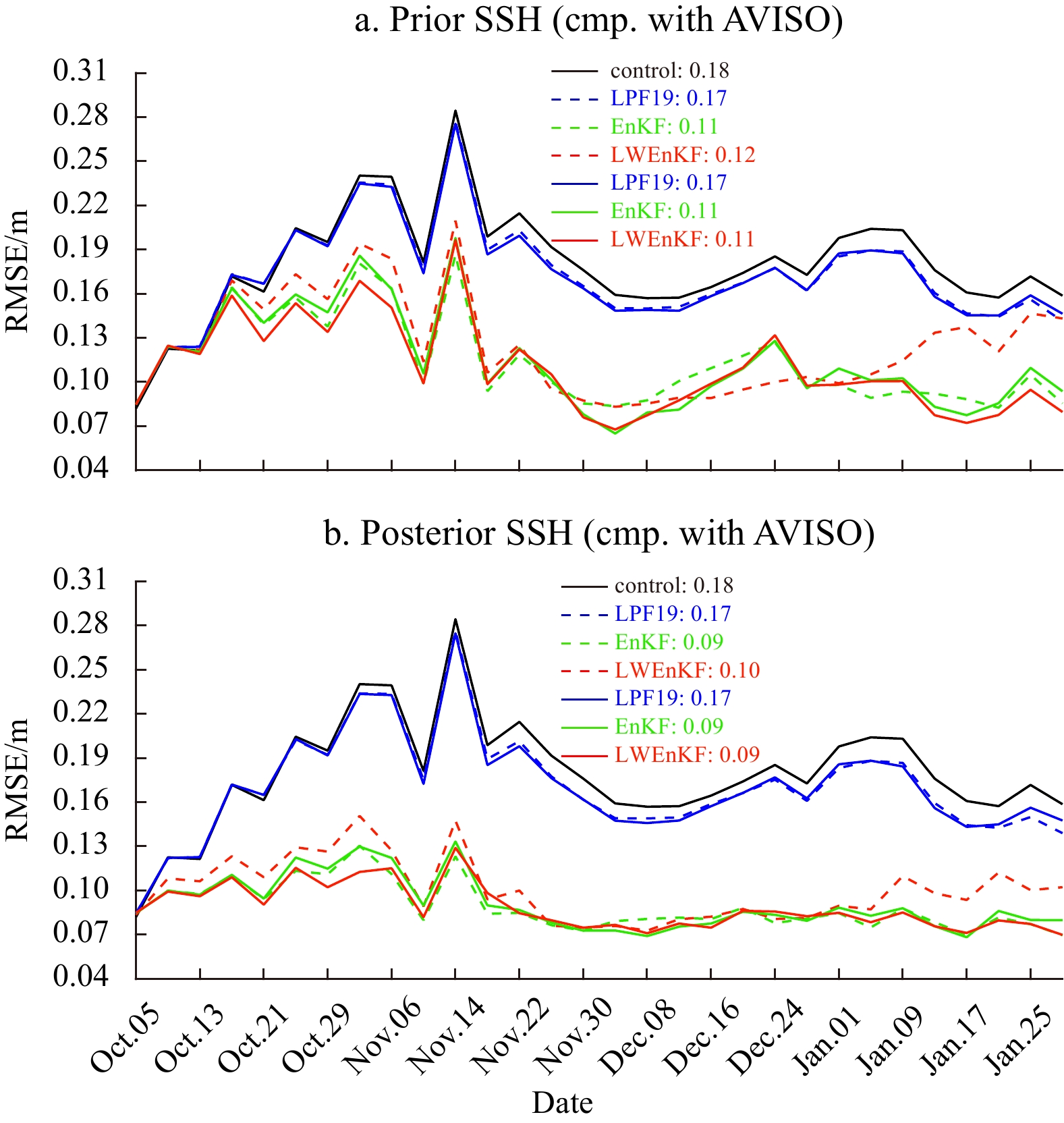
The assimilation of both AT-SSH and S-SST does not show a better effect than AT-SSH assimilation alone based on the RMSE time series and the statistical average RMSE results. This result indicates that S-SST assimilation has a limited influence on the SSH simulation, as opposed to the positive effect of AT-SSH assimilation on SST simulation. For AT-SSH assimilation alone, the LWEnKF does not have the same effect as the EnKF, but the LWEnKF can be comparable to the EnKF for both AT-SSH and S-SST assimilation.
Whether considering single variable assimilation or joint variable assimilation, the LPF19 is not ideal for the simulation of SST and SSH. The assimilation effects of the EnKF and LWEnKF are much better than those of the LPF19. For SSH and SST prediction and analysis, the LWEnKF performs no worse than the EnKF.
ExpE assimilates EN4.2.1 T/S profiles, including T/S profiles from both Argo and CTD and temperature profiles from XBT. There are 577 T/S profiles in total, of which 446 are from Argo. The locations of all the profiles are marked in Fig.1 with red points. The Argo data are uniformly distributed in the whole assimilation period, and the data from XBT and CTD are less. The T/S profiles from Argo are used to validate the performance of the assimilation system. The RMSEs of T/S profiles are calculated to evaluate the performance of different assimilation methods.
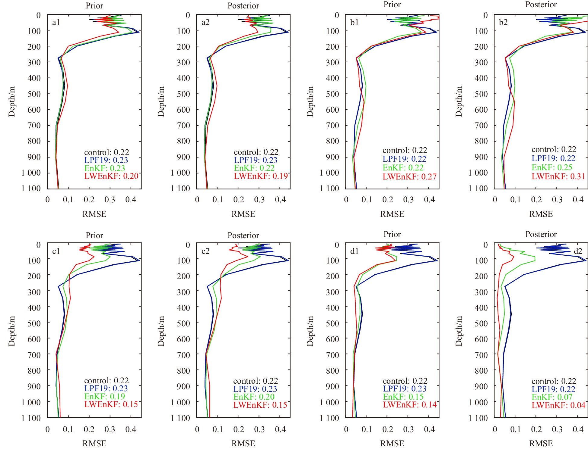
Figure 5 shows the RMSEs of the temperature profiles. It should be noted that no matter what data are assimilated, there is no significant difference between the results of LPF (blue lines) and those of the control test (black lines), and assimilation does not affect. Hence the focus is only put on EnKF and LWEnKF hereafter.

In the experiment of AT-SSH assimilation only (Fig. 5b), the prior and posterior results are not as good as the control experiment above 200 m, and AT-SSH does not bring positive adjustment to the internal ocean temperature. When S-SST is only assimilated (Fig. 5a), the temperature field in the upper layer of the ocean is well constrained, and there is no similar situation with AT-SSH only assimilated, and the temperature field in the internal ocean is well adjusted. Compared to the control experiment, the RMSEs decrease above 200 m when assimilating AT-SSH and S-SST together (Fig. 5c). When all the data including T/S profiles are assimilated (Fig. 5d), the RMSE curves of the EnKF and LWEnKF have roughly the same shapes. The RMSE values increase with depth and reach the maximum value near 150 m depth. Below 150 m, RMSE values decrease with increasing depth. When comparing the three methods, the EnKF and LWEnKF are shown to be significantly better than the LPF19, and the LWEnKF has the smallest mean RMSE. The LWEnKF is significantly better than the EnKF at depths below 100 m and is equivalent to the EnKF at depths of above 100 m. In terms of posterior RMSE, LWEnKF and EnKF assimilation remarkably adjust the prior field, while the LPF19 assimilation effect is not visible. From the average RMSEs, for the prior, the LWEnKF reduces by 22.63% compared to the EnKF, and for the posterior, it reduces by 55.11%.
Figure 6 shows the RMSEs of the salinity profiles. The significant feature of the RMSE curves is that they fluctuate greatly in the upper layer. The experiments conducted in this study do not assimilate sea surface salinity (SSS) data. Compared to temperature data assimilation, the results of the model deviate from the actual upper ocean salinity without the constraint of SSS observations. The model is unstable after the assimilation of the salinity profiles, and the RMSE fluctuates at depths of shallower than 100 m. However, under the constraint of S-SST data, the RMSE of the temperature profiles does not have similar instability.

No matter what data are assimilated, there is no improvement in the salinity field for LPF compared with the control experiment. The results of EnKF and LWEnKF are not much better than those of the control experiment when AT-SSH (Fig. 6a) or S-SST (Fig. 6b) are assimilated alone. The situation improves slightly when S-SST and AT-SSH are assimilated together (Fig. 6c). EnKF and LWEnKF show a slightly better prediction effect than the control experiment above 200 m and LWEnKF is obviously better than EnKF.
When all the data including T/S profiles are assimilated (Fig. 6d), the LWEnKF has the smallest mean RMSE, and its effect is better than that of the EnKF at depths of below 100 m. From the posterior RMSE, the assimilations of the LWEnKF and EnKF make visible adjustments to the forecast, and the effect of the LPF19 assimilation seems null (also see in Fig. 7) and therefore the results from LPF19 will not be discussed hereafter. From the average RMSEs, for the prior, the LWEnKF reduces by 11.58% compared to the EnKF, and for the posterior, it reduces by 35.22%.

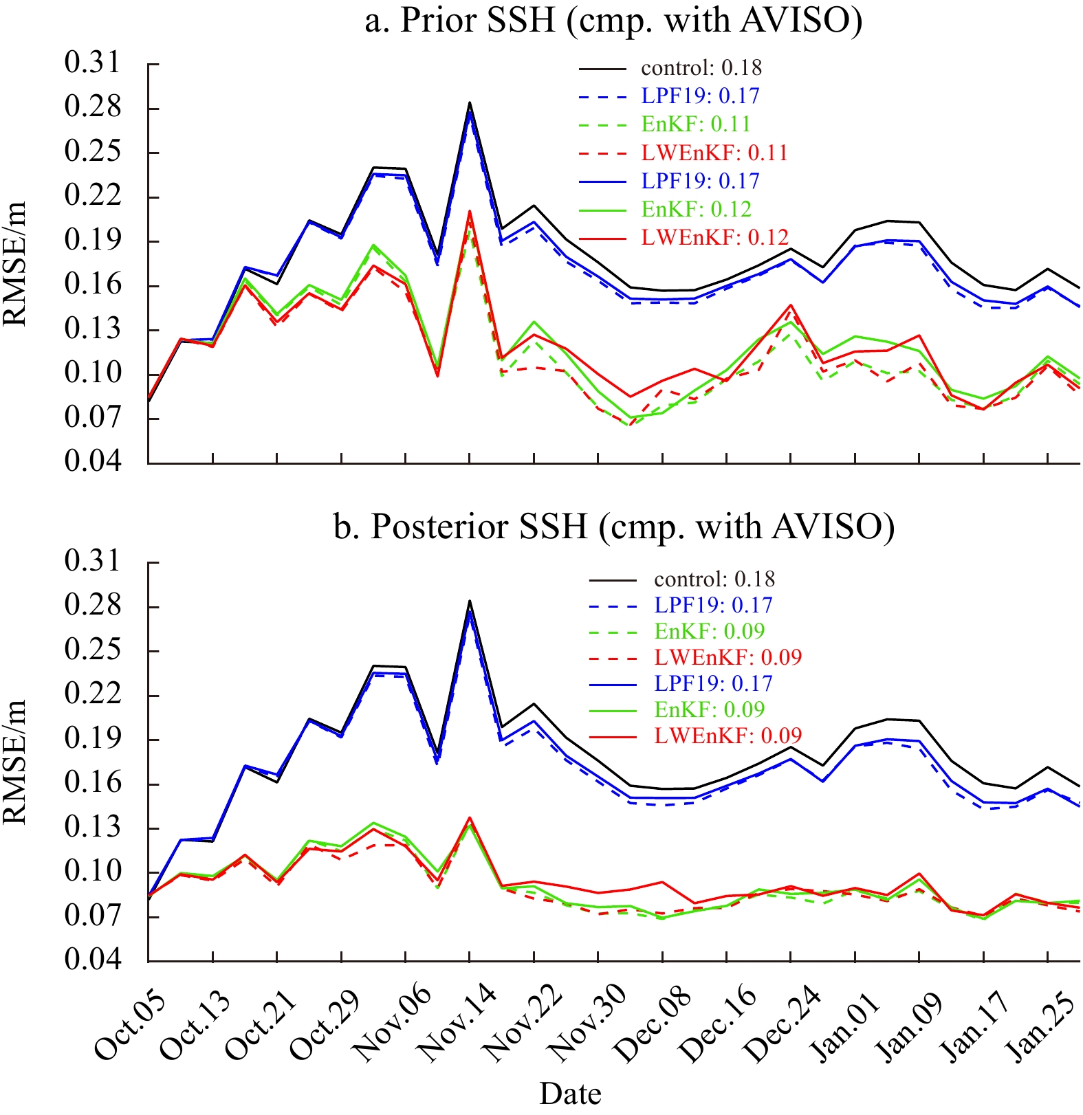
To explore the changes brought by the assimilation of T/S profiles to SSH, the RMSEs of SSH are shown in Fig. 7. There is no significant difference in the RMSEs of SSH before and after T/S profiles assimilation. From the RMSEs values, the effect of the assimilation of the T/S profiles on SSH is limited. It may be because the T/S profiles are too sparse for the model domain, and it is difficult to make obvious adjustments to SSH.
To display the sea surface state more intuitively and verify the prediction performance of the assimilation system, the results from ExpE1 and ExpE2 are compared with the result from ExpA as well as the grid data products on the following three dates: (1) December 4, 2013, when the warm eddy was generated and in a stable stage; (2) December 28, 2013, when the cold and warm eddy coexisted and (3) January 17, 2014, when the cold and warm eddy development process was in the last stage.
Figure 8 shows the SLA distribution and sea surface currents. The red dots in Figs 8d–f represent the locations of assimilated AT-SSH data of the previous time window. The LWEnKF and EnKF assimilation systems have slightly different sea surface states, but either system successfully predicts the cold and warm eddy processes. In the initial stage of warm eddy generation on December 4, 2013, compared with AVISO SLAs, the forecasted SLAs of the two systems are weaker, but the distribution ranges are more widespread than that of AVISO SLA. Compared to that of the EnKF, the forecasted warm eddy of the LWEnKF is closer to that of AVSIO. The currents near the warm eddy predicted by the EnKF are weaker than those predicted by OSCAR, and the currents on the west side of the warm eddy predicted by the LWEnKF are slightly weaker than that of OSCAR. The characteristics of the flow field clearly show that the warm eddy is probably the result of the Kuroshio current crossing the Luzon Strait and invading the SCS. Previous studies have shown that warm and cold eddies are often accompany each other (Nan et al., 2011). Zhang et al. (2013) discussed the formation mechanism of a cold eddy on the back edge of a warm eddy in detail.

On December 28, 2013, a cold and warm eddy pair appeared, and the shapes of the cold and warm eddies were stable. The LWEnKF and EnKF systems forecasted the cold eddy well. Compared to AVISO SLA, the EnKF forecasts show a weak cold eddy, while the LWEnKF and AVISO show similar cold eddy strengths. For the currents near the cold eddy, the LWEnKF forecast is in good agreement with OSCAR, and the performance of the EnKF forecast is generally poor. Neither the LWEnKF method nor the EnKF method are ideal for the prediction of the warm eddy, which is much weaker in the LWEnKF and EnKF than in AVISO, and the warm eddy predicted by the EnKF nearly disappears. Moreover, the prediction results of the two methods show that there are two large-scale cyclonic eddies in the southern part of the study area, which are much larger than the cyclonic eddy on the east side of Luzon Island in the AVISO SLA. This phenomenon is caused by the uneven spatial distribution of assimilated AT-SSH. The observed distribution is sparse in the sea, and assimilation cannot effectively constrain the models. According to the locations (red dots) of assimilated AT-SSH data in the previous time window, the observation distribution is relatively sparse in the area in which the prediction effect is not ideal.
The warm eddy moved southwest along the continental shelf. On January 7, 2014, the shape of the warm eddy remained stable, and the cold eddy had a tendency to converge with the large-scale cold eddy in the south, but its structure was still stable. The LWEnKF effectively predicted the state of cold and warm eddies at this time, and its currents corresponded well to those of OSCAR. The strength of the forecasted cold eddy was slightly stronger than that of AVISO. By comparison, the prediction effect of the EnKF was not ideal, the warm eddy basically disappeared, and the cold eddy was nearly extinct. Without observations constraints, the prediction results of the control experiment (Figs 8j–i) are not ideal and are significantly different from the grid data. In comparison, the prediction effect of the LWEnKF assimilation system is remarkable.
Figure 9 shows the SST corresponding to SLA for three days. In initial stages of the formation of the warm eddy on December 4, 2013, the high-temperature region in the center of the warm eddy predicted by the two methods shows a good correspondence with that of the AVHRR. On December 28, 2013, cold and warm eddy structures can be observed from the AVHRR SST, and the LWEnKF prediction results show the corresponding low-temperature structure in the center of the cold eddy. However, the cold eddy intensity is weaker in the LWEnKF than in the AVHRR, and the high-temperature structure of the predicted warm eddy is not significant. It is difficult to observe the cold and warm eddy structures in the EnKF prediction results, and its predictions are not ideal. On January 7, 2014, the cold eddy structure of the AVHRR SST was stable, and the high-temperature structure of the warm vortex was clearly visible. The low-temperature structure of the cold eddy can be observed from the LWEnKF forecast results, and the strength of the cold eddy in LWEnKF is weaker than that in the AVHRR. However, the prediction results do not capture the characteristics of warm eddies. Although the temperature field predicted by the EnKF corresponds well with the AVHRR in most sea areas, the EnKF fails to predict the temperature structures of cold and warm eddies. The prediction effect of control experiment is obviously different from the grided data.

Based on the current, SLA and SST distributions, the LWEnKF system can accurately predict the surface structure characteristics of mesoscale eddies.
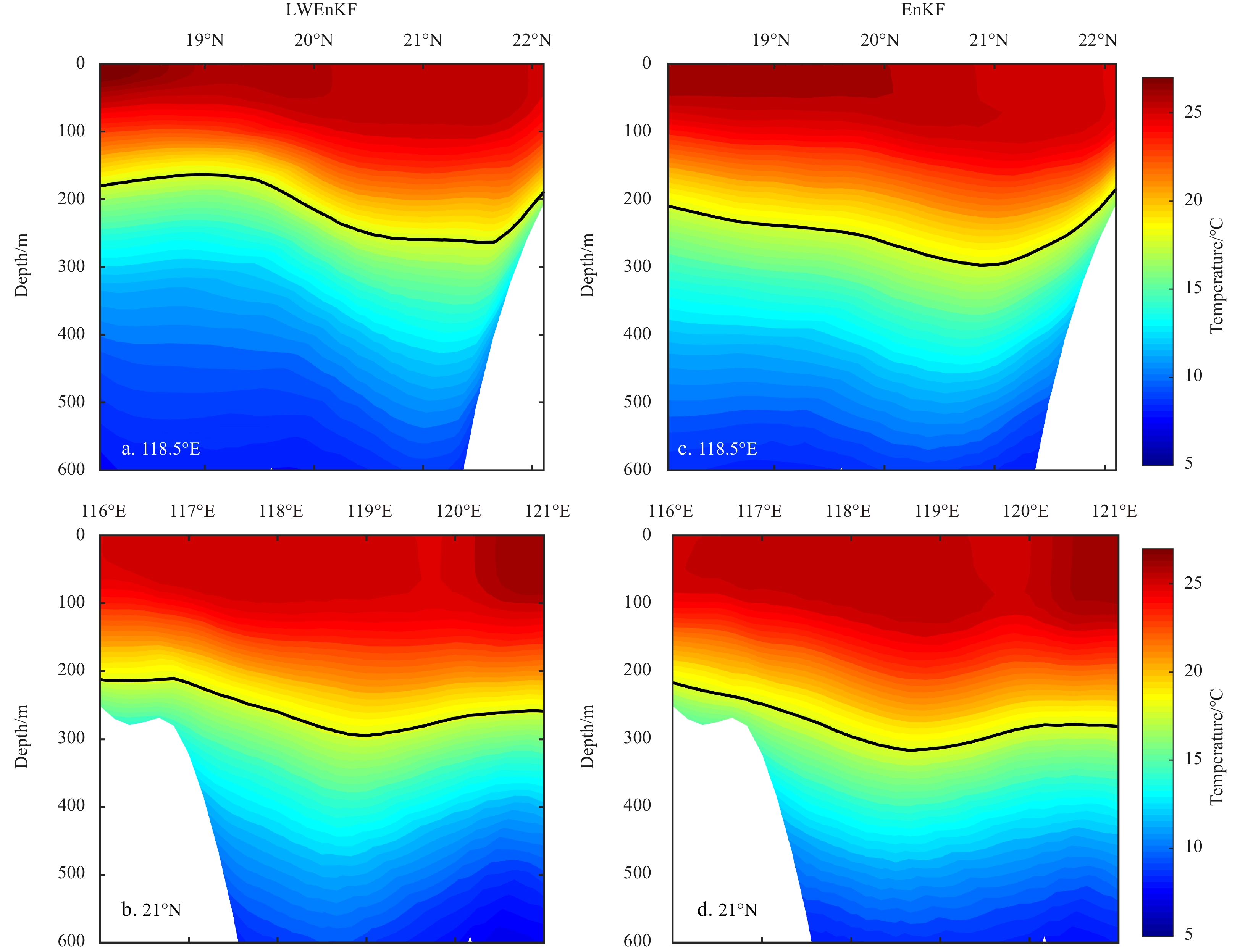
A mesoscale warm eddy, which was found stable from its surface structure on December 4, 2013 (Fig. 8a), ranging from 19°–22°N and 117°–121°E, is specifically extracted to compare the performance among different assimilation experiments. Figure 10 shows the prediction results of the ExpB3, ExpC3, ExpE1 and ExpE2 in this region. Due to the low vertical resolution of the model, the results are only shown above 600 m.

Figure 10 shows the horizontal distribution of temperature at different depths, i.e., the three-dimensional structure. The high-temperature region of the warm eddy can be clearly seen at different depths from the results of the LWEnKF forecast (Figs 10a–f). The high-temperature center of the warm eddy is not consistent at different depths, and the high-temperature center gradually deviates to the southwest from the 200 m layer to the 600 m layer. The warm eddy is tilted down to the southwest vertically, and the direction of tilt is consistent with the direction of warm eddy motion. According to Zhang et al. (2016), this tilted structure of the mesoscale eddy in the SCS is related to the terrain of the continental slope. Due to the topographic
The temperature slices of no assimilation of T/S profiles are shown in Figs 10m–x. Compared them with the forecast results of LWEnKF (Figs 10a-f), the difference is quite obvious. From the RMSEs of the vertical temperature profiles (Fig. 5), both schemes (LWEnKF and EnKF) have better performance after assimilating additional T/S profiles. Furthermore, compared with the result from adopting the EnKF scheme, the predicated temperature field among 100−600 m shows smaller RMSEs when using the LWEnKF scheme, whereas both schemes assimilate additional T/S profiles.
Figures 11 and 12 show the temperature and potential density section of the warm eddy on December 4, respectively, which are the forecast results of ExpE1 and ExpE2. The longitude and latitude correspond to the dotted white lines in Fig. 10 (21°N, 118.5°E). Both temperature and potential density isolines tend to deepen in the eddy region. The solid black lines in Fig. 11 indicate the 18°C isotherm and represent the location of the thermocline. Zhang et al. (2013) captured this warm eddy process through mooring array observations. The time series of temperature obtained by his observations showed that the 18°C isotherm was between 100 m and 200 m depth before the warm eddy arrived, and the isotherm was close to 250 m depth when the eddy passed. According to the 18°C isotherm shown in Fig. 11, the depth of the thermocline predicted by the EnKF is deeper than that of the LWEnKF, and the LWEnKF is more consistent with the actual observations given by Zhang et al. (2016). The potential density can reflect the properties of water masses. Figure 12 shows significant changes in potential density in the eddy area. The warm eddy water has unique properties of temperature and salinity.

The mesoscale warm eddy process is closely related to the Kuroshio current flowing through the Luzon Strait, from the perspective of only surface currents. Previous studies based on sea surface state suggest that the Kuroshio current often invades the SCS in the form of a loop current when flowing through the Luzon Strait and is often accompanied by spinoff or detaching of a warm mesoscale eddy (Caruso et al., 2006; Jia and Chassignet, 2011).
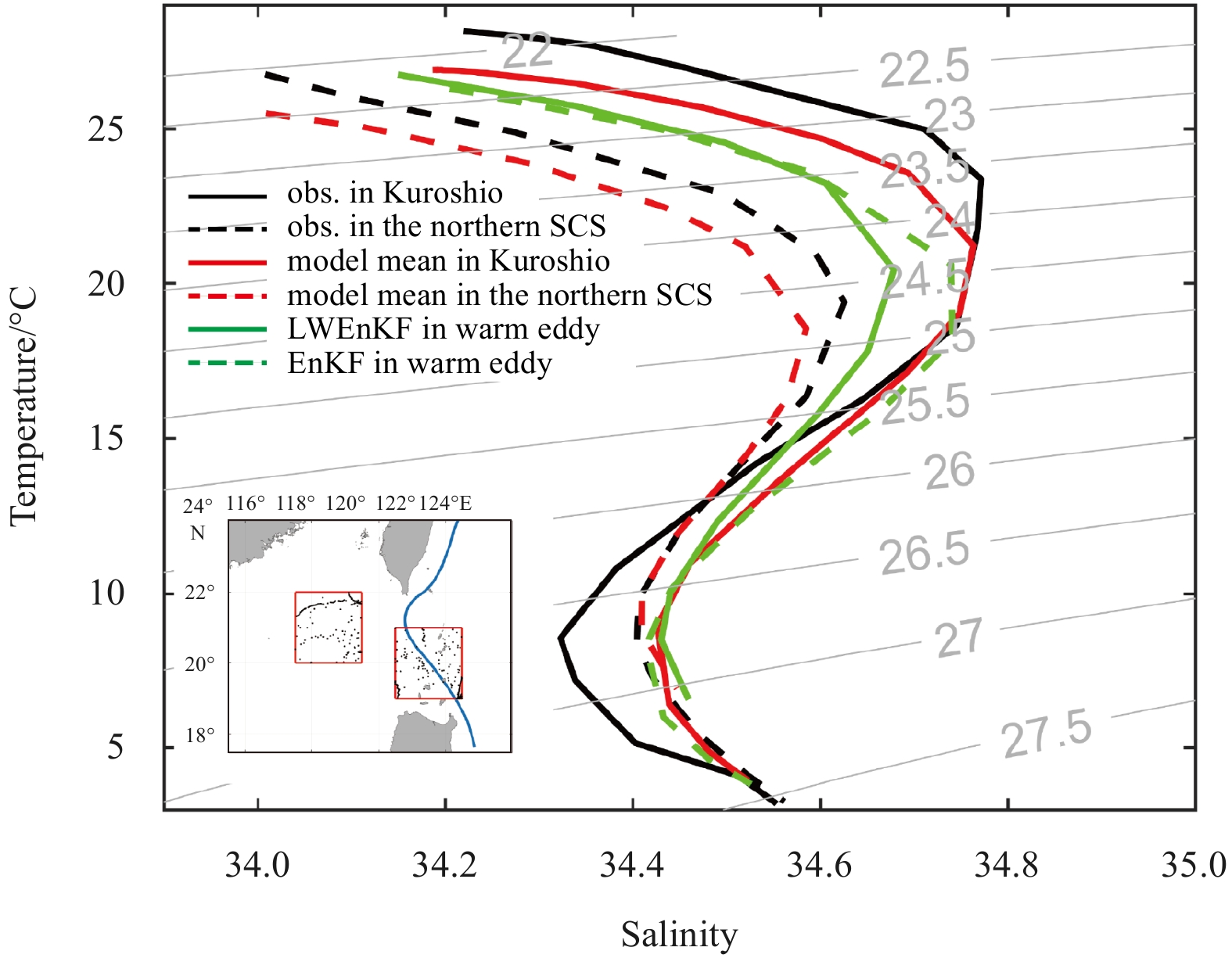
The water mass properties of the SCS and Kuroshio current is considered to explore the source of the mesoscale warm eddy. Figure 13 shows T/S diagrams of the water masses from the SCS (20°–22°N, 117.5°–119.5°E) and the Kuroshio Current along the Luzon Strait (19°–21°N, 120.5°–122.5°E). The black lines in Fig. 13 show the average of all salinity and temperature profiles of the EN4.2.1 dataset for 2011 to 2014. From the observations of the temperature and salinity properties, there are obvious differences between Kuroshio and SCS waters. The former shows the characteristics of high temperature and high salinity in the surface and subsurface water, and its maximum salinity can reach 34.8. The middle layer is characterized by low temperature and low salinity, and the lowest salinity reaches 34.3. Although the SCS water shows a similar S-shaped curve, its maximum salinity in the subsurface layer is only 34.6, and its minimum salinity in the middle layer is greater than 34.4. The red lines in Fig. 13 are the averages of the LWEnKF system forecast results from October 3, 2013 to February 1, 2014. T/S diagrams obtained from the forecast are consistent with historical observations and can reflect the temperature and salinity characteristics of Kuroshio and SCS waters.

The green solid line shows the T/S diagram of the warm eddy region (20°–22°N, 117.5°–119.5°E) predicted by the LWEnKF system for December 4, 2013. The T/S diagram of warm eddy water is positioned between those of Kuroshio and SCS waters, and the temperature and salinity characteristics of warm eddy water have properties of mixed Kuroshio and SCS waters. This is consistent with the conclusion that warm eddy water breaks off from the Kuroshio Current, enters the SCS and mixes with SCS water. This result is also consistent with the observations of Zhang et al. (2016) in the SCS, and the LWEnKF system prediction results are reasonable. The green dotted line shows the results of the EnKF. However, near the thermocline (potential density 24–25), the warm eddy mixing property predicted by the EnKF is not obvious. Compared with the LWEnKF, the EnKF shows the characteristics of high temperature and high salt, which also correspond to the previous observation results of temperature slices.
In the along-track satellite data assimilation experiment conducted in this paper, the LWEnKF was found to be significantly better than the LPF19, and the effect of the LWEnKF was found to be comparable to that of the EnKF only from the statistical RMSE results of SST and SLA tests. However, based on the distributions of SLA, SST and surface ocean currents, the LWEnKF prediction results are more reasonable than the EnKF prediction results. In this study, velocity observations were not assimilated. For unobserved variables, the EnKF represents the relationship between different state variables through covariance and cannot consider the information of higher-order moments (such as kurtosis and skewness). The LWEnKF estimates the complete PDF by particle weight and can obtain more accurate posterior state variables than the EnKF. The theoretical advantages of the LWEnKF are reflected in this study.
Based on the vertical coordinates of the ROMS model, a vertical localization radius function is designed for the assimilation of T/S profiles. Although this function is introduced in all three assimilation systems, the LWEnKF has the best prediction and assimilation effect for the temperature and salinity fields in the ocean based on the vertical distribution of RMSE values. The RMSE values near the thermocline (100–200 m) are relatively large, which may be due to the simulated temperature and salinity fields near the thermocline deviating from actual conditions. Based on only the statistical RMSE results, the assimilation can significantly improve the prediction, but the prediction effect near the thermocline is not ideal.
The LWEnKF assimilation system has successfully predicted the mesoscale warm eddy process and has a good description of the temperature structure of the eddy above 600 m depth. This warm eddy is vertically tilted down toward the southwest, which is due to the topographic
The prediction effect of the LPF19 assimilation system is not ideal, and the assimilation does not significantly improve the initial state field of the model, although the localization parameter
Notably, the uneven spatial distribution of observations has a significant impact on the prediction effect. For AT-SSH, there are only three altimeter satellite datasets during the whole assimilation period. The observations within one assimilation window do not uniformly cover the whole sea, and the sparsity of observations affects the prediction ability. The LWEnKF shows stronger adaptability than the EnKF for heterogeneous observations. Nevertheless, it is meaningful to conduct further research on the influence of the spatial distribution of observations on prediction ability under the framework of the LWEnKF.
Thanks to Ding Liu for providing the axis of Kuroshio.
| [1] |
Anderson J L. 2003. A local least squares framework for ensemble filtering. Monthly Weather Review, 131(4): 634–642. doi: 10.1175/1520-0493(2003)131<0634:ALLSFF>2.0.CO;2
|
| [2] |
Anderson J L. 2007. An adaptive covariance inflation error correction algorithm for ensemble filters. Tellus A, 59(2): 210–224. doi: 10.1111/j.1600-0870.2006.00216.x
|
| [3] |
Bonjean F, Lagerloef G S E. 2002. Diagnostic model and analysis of the surface currents in the tropical Pacific Ocean. Journal of Physical Oceanography, 32(10): 2938–2954. doi: 10.1175/1520-0485(2002)032<2938:DMAAOT>2.0.CO;2
|
| [4] |
Caruso M J, Gawarkiewicz G G, Beardsley R C. 2006. Interannual variability of the Kuroshio intrusion in the South China Sea. Journal of Oceanography, 62(4): 559–575. doi: 10.1007/s10872-006-0076-0
|
| [5] |
Chen Yan, Zhang Weimin, Wang Pinqiang. 2020a. An application of the localized weighted ensemble Kalman filter for ocean data assimilation. Quarterly Journal of the Royal Meteorological Society, 146(732): 3029–3047. doi: 10.1002/qj.3824
|
| [6] |
Chen Yan, Zhang Weimin, Zhu Mengbin. 2020b. A localized weighted ensemble Kalman filter for high-dimensional systems. Quarterly Journal of the Royal Meteorological Society, 146(726): 438–453. doi: 10.1002/qj.3685
|
| [7] |
Chustagulprom N, Reich S, Reinhardt M. 2016. A hybrid ensemble transform particle filter for nonlinear and spatially extended dynamical systems. SIAM/ASA Journal on Uncertainty Quantification, 4(1): 592–608. doi: 10.1137/15M1040967
|
| [8] |
Farchi A, Bocquet M. 2018. Review article: comparison of local particle filters and new implementations. Nonlinear Processes in Geophysics, 25(4): 765–807. doi: 10.5194/npg-25-765-2018
|
| [9] |
Gaspari G, Cohn S E. 1999. Construction of correlation functions in two and three dimensions. Quarterly Journal of the Royal Meteorological Society, 125(554): 723–757. doi: 10.1002/qj.49712555417
|
| [10] |
Good S A, Martin M J, Rayner N A. 2013. EN4: quality controlled ocean temperature and salinity profiles and monthly objective analyses with uncertainty estimates. Journal of Geophysical Research: Oceans, 118(12): 6704–6716. doi: 10.1002/2013JC009067
|
| [11] |
Hoteit I, Hoar T, Gopalakrishnan G, et al. 2013. A MITgcm/DART ensemble analysis and prediction system with application to the Gulf of Mexico. Dynamics of Atmospheres and Oceans, 63: 1–23. doi: 10.1016/j.dynatmoce.2013.03.002
|
| [12] |
Hoteit I, Pham D T, Triantafyllou G, et al. 2008. A new approximate solution of the optimal nonlinear filter for data assimilation in meteorology and oceanography. Monthly Weather Review, 136(1): 317–334. doi: 10.1175/2007MWR1927.1
|
| [13] |
Ingleby B, Huddleston M. 2007. Quality control of ocean temperature and salinity profiles -historical and real-time data. Journal of Marine Systems, 65(1–4): 158–175.
|
| [14] |
Jia Yinglai, Chassignet E P. 2011. Seasonal variation of eddy shedding from the Kuroshio intrusion in the Luzon Strait. Journal of Oceanography, 67(5): 601–611. doi: 10.1007/s10872-011-0060-1
|
| [15] |
Lee Y, Majda A J. 2016. State estimation and prediction using clustered particle filters. Proceedings of the National Academy of Sciences of the United States of America, 113(51): 14609–14614. doi: 10.1073/pnas.1617398113
|
| [16] |
Li Yi, Toumi R. 2017. A balanced Kalman filter ocean data assimilation system with application to the South Australian Sea. Ocean Modelling, 116: 159–172. doi: 10.1016/j.ocemod.2017.06.007
|
| [17] |
Metzger E J, Smedstad O M, Thoppil P G, et al. 2014. US Navy operational global ocean and Arctic ice prediction systems. Oceanography, 27(3): 32–43. doi: 10.5670/oceanog.2014.66
|
| [18] |
Nan Feng, Xue Huijie, Xiu Peng, et al. 2011. Oceanic eddy formation and propagation southwest of Taiwan. Journal of Geophysical Research: Oceans, 116(C12): C12045. doi: 10.1029/2011JC007386
|
| [19] |
Papadakis N, Mémin E, Cuzol A, et al. 2010. Data assimilation with the Weighted Ensemble Kalman Filter. Tellus A, 62(5): 673–697. doi: 10.1111/j.1600-0870.2010.00461.x
|
| [20] |
Penny S G, Miyoshi T. 2016. A local particle filter for high-dimensional geophysical systems. Nonlinear Processes in Geophysics, 23(6): 391–405. doi: 10.5194/npg-23-391-2016
|
| [21] |
Pham D T. 2001. Stochastic methods for sequential data assimilation in strongly nonlinear systems. Monthly Weather Review, 129(5): 1194–1207. doi: 10.1175/1520-0493(2001)129<1194:SMFSDA>2.0.CO;2
|
| [22] |
Poterjoy J. 2016. A localized particle filter for high-dimensional nonlinear systems. Monthly Weather Review, 144(1): 59–76. doi: 10.1175/MWR-D-15-0163.1
|
| [23] |
Poterjoy J, Wicker L, Buehner M. 2019. Progress toward the application of a Localized Particle Filter for numerical weather prediction. Monthly Weather Review, 147(4): 1107–1126. doi: 10.1175/MWR-D-17-0344.1
|
| [24] |
Rebeschini P, van Handel R. 2015. Can local particle filters beat the curse of dimensionality?. The Annals of Applied Probability, 25(5): 2809–2866
|
| [25] |
Sebastien B, Anne C, Sai S G, et al. 2013. Weighted ensemble transform Kalman filter for image assimilation. Tellus A, 65(1): 18803. doi: 10.3402/tellusa.v65i0.18803
|
| [26] |
Shen Zheqi, Tang Youmin, Gao Yanqiu. 2016. The theoretical framework of the ensemble-based data assimilation method and its prospect in oceanic data assimilation. Haiyang Xuebao (in Chinese), 38(3): 1–14
|
| [27] |
Shen Zheqi, Tang Youmin, Li Xiaojing. 2017. A new formulation of vector weights in localized particle filters. Quarterly Journal of the Royal Meteorological Society, 143(709): 3269–3278. doi: 10.1002/qj.3180
|
| [28] |
van Leeuwen P J, Cheng Yuan, Reich S. 2015. Nonlinear Data Assimilation. Cham: Springer, 31–41
|
| [29] |
van Leeuwen P J, Künsch H R, Nerger L, et al. 2019. Particle filters for high-dimensional geoscience applications: a review. Quarterly Journal of the Royal Meteorological Society, 145(723): 2335–2365. doi: 10.1002/qj.3551
|
| [30] |
Wang Pinqiang, Zhu Mengbin, Chen Yan, et al. 2020. Implicit equal-weights Variational particle smoother. Atmosphere, 11(4): 338. doi: 10.3390/atmos11040338
|
| [31] |
Wang Pinqiang, Zhu Mengbin, Chen Yan, et al. 2021. Ocean satellite data assimilation using the implicit equal-weights variational particle smoother. Ocean Modelling, 164: 101833. doi: 10.1016/j.ocemod.2021.101833
|
| [32] |
Zhang Zhiwei, Tian Jiwei, Qiu Bo, et al. 2016. Observed 3D structure, generation, and dissipation of oceanic Mesoscale eddies in the South China Sea. Scientific Reports, 6(1): 24349. doi: 10.1038/srep24349
|
| [33] |
Zhang Yongchui, Wang Ning, Zhou Lin, et al. 2020. The surface and three-dimensional characteristics of mesoscale eddies: a review. Advances in Earth Science, 35(6): 568–580
|
| [34] |
Zhang Zhiwei, Zhao Wei, Tian Jiwei, et al. 2013. A mesoscale eddy pair southwest of Taiwan and its influence on deep circulation. Journal of Geophysical Research: Oceans, 118(12): 6479–6494. doi: 10.1002/2013JC008994
|
| 1. | Raquel Toste, Carina Stefoni Böck, Maurício Soares da Silva, et al. CODAR data assimilation into an integrated ocean forecasting system for the Brazilian Southeastern coast. Ocean Modelling, 2024, 188: 102331. doi:10.1016/j.ocemod.2024.102331 | |
| 2. | Zheming Pang, Yajun Wang, Fang Yang. Application of optimized Kalman filtering in target tracking based on improved Gray Wolf algorithm. Scientific Reports, 2024, 14(1) doi:10.1038/s41598-024-59610-6 | |
| 3. | Huizan Wang, Yan Chen, Weimin Zhang. Some progress on ocean data assimilation in China: Introduction of the special section “Ocean Data Assimilation”. Acta Oceanologica Sinica, 2022, 41(2): 1. doi:10.1007/s13131-021-1982-0 |

Figures(13) / Tables(1)

Supported by:
Beijing Renhe Information Technology Co. Ltd

Meng Shen, Yan Chen, Pinqiang Wang, Weimin Zhang. Assimilating satellite SST/SSH and in-situ T/S profiles with the Localized Weighted Ensemble Kalman Filter[J]. Acta Oceanologica Sinica, 2022, 41(2): 26-40. doi: 10.1007/s13131-021-1903-2

| Experiment | Method | Assimilated variables |
| ExpA | Control run | none |
| ExpB1 | LWEnKF | AT-SSH |
| ExpB2 | S-SST | |
| ExpB3 | AT-SSH, S-SST | |
| ExpC1 | EnKF | AT-SSH |
| ExpC2 | S-SST | |
| ExpC3 | AT-SSH, S-SST | |
| ExpD1 | LPF19 | AT-SSH |
| ExpD2 | S-SST | |
| ExpD3 | AT-SSH, S-SST | |
| ExpE1 | LWEnKF | AT-SSH, S-SST, T/S profiles |
| ExpE2 | EnKF | AT-SSH, S-SST, T/S profiles |
| ExpE3 | LPF19 | AT-SSH, S-SST, T/S profiles |
DownLoad:
CSV
 DownLoad:


 DownLoad: