Li Gao, Yingbin Wang. Influences of environmental factors on the spawning stock-recruitment relationship of Portunus trituberculatus in the northern East China Sea[J]. Acta Oceanologica Sinica, 2021, 40(8): 145-159. doi: 10.1007/s13131-021-1801-7
Citation:
Li Gao, Yingbin Wang. Influences of environmental factors on the spawning stock-recruitment relationship of Portunus trituberculatus in the northern East China Sea[J]. Acta Oceanologica Sinica, 2021, 40(8): 145-159. doi: 10.1007/s13131-021-1801-7
Li Gao, Yingbin Wang. Influences of environmental factors on the spawning stock-recruitment relationship of Portunus trituberculatus in the northern East China Sea[J]. Acta Oceanologica Sinica, 2021, 40(8): 145-159. doi: 10.1007/s13131-021-1801-7
Citation:
Li Gao, Yingbin Wang. Influences of environmental factors on the spawning stock-recruitment relationship of Portunus trituberculatus in the northern East China Sea[J]. Acta Oceanologica Sinica, 2021, 40(8): 145-159. doi: 10.1007/s13131-021-1801-7
School of Fishery, Zhejiang Ocean University, Zhoushan 316022, China
Funds:
The National Key Research and Development Program of China under contract Nos 2017YFA0604902 and 2019YFD0901304; the Public Welfare Technology Application Research Project of Zhejiang under contract No. LGN21C190009.
Based on the Ricker-type models, the spawning stock-recruitment (S-R) relationship of Portunus trituberculatus was analysed under the impacts of environmental factors (including red tide area (AORT), sea level height (SLH), sea surface salinity (SSS) and typhoon landing times (TYP)) in the northern East China Sea in 2001 and 2014. Besides the traditional Ricker model, two other Ricker-type S-R models were built: Ricker model with ln-linear environmental impact (Ricker-type 2) and Ricker model with ln-quadratic polynomial environmental impact (Ricker-type 3). Results showed that AORT, SLH, SSS and TYP had great influences on the recruitment of P. trituberculatus. When SSS reached 29 and 31, recruitment decreased from 20.7×10³ million to 8.3×10³ million individuals. In this case, recruitment declined, whereas AORT and TYP increased. Analysis of the S-R model showed that the Akaike information criterion (AIC) value of the traditional Ricker model was 14.619, which remarkably decreased after addition of the environmental factors. Different numbers of environmental factors were added to the Ricker model, and the best result was obtained when four factors were added to the model together. Moreover, Ricker-type 2 model, with the AIC value of −5.307, was better than Ricker-type 3 model (add above four environmental factors at the same time). The findings indicated that the mechanisms by which various environmental factors affect the S-R relationship are different.
Portunus trituberculatus is the most widely fished crab, accounts for one-quarter of the crab caught commercially worldwide (Liu et al., 2013) and is amongst the most important economic species in China, especially in the East China Sea. The P. trituberculatus catch in the East China Sea accounts for 50% of the total yield of the three main fishing areas of the East China Sea, the Yellow Sea, and the Bohai Sea (Song et al., 2012). The northern East China Sea is the largest production area of P. trituberculatus in the East China Sea and yields over 40% of the total catch (Yu et al., 2003). The P. trituberculatus catch in the northern East China Sea has increased continuously since 2010, which indicates that the recruitment stock (R) of this crab may significantly increase. In 2017, the Ministry of Agriculture of the PRC decided to carry out a pilot project for the total allowable catch management of P. trituberculatus in the northern Zhejiang fishing ground. Thus, scientific stock assessment of this species in the study area is very important and necessary.
In order to give scientific assessment results and management recommendations for P. trituberculatus, it is essential to have knowledge of the spawning stock-recruitment (S-R) relationship (Myers, 2002) and the estimations of S-R relationship are also an important part of the development of an optimal harvest strategy (Zheng and Kruse, 2003). Scientists believe that a higher spawning stock biomass (S) does not necessarily lead to abundant recruitment (Myers et al., 1996), which indicates that recruitment may be independent of the spawning stock. Considering that recruitment represents survivors suffering from different environmental conditions, the effects of environmental factors on recruitment may be stronger than those effects of the spawning stock. Therefore, interest in environmental impacts on recruitment continuous to increase. Sakuramoto (2013) indicates that introducing environmental factors to the S-R relationship model is necessary to better understand fish population dynamics. Several research studies also show that changes in the marine environment determine the distribution of Ommastrephidae resources to some extent (Anderson and Rodhouse, 2001; Palacios et al., 2006). Environmental factors, such as water temperature, interfere with the population compensation of Thunnus albacares (Feng et al., 2010).
The Ricker S-R model, which was proposed in 1954, has been frequently used to study the relationship between spawning stock and recruitment (Hilborn and Walters, 1992). It was also used to study the effects of environmental factors on the S-R relationship (Pécuchet et al., 2015). For instance, Lin et al. (2018) studies the influence of sea surface temperature and Pacific decadal oscillation on the spawning and recruitment of Scomber japonicus and compared the performance of Ricker models with one and two environmental factors. Results show that Ricker models with two environmental factors can accurately describe the S-R relationship (Lin et al., 2018). Many similar studies are also conducted on the effects of environmental factors on S-R relationships by using Ricker-type models (Galindo-Cortes et al., 2010; Shih et al., 2014).
It is reported that the abundance and catch of P. trituberculatus in the East China Sea are affected by environmental factors (Wang et al., 2017a, 2017b). The recruitment of P. trituberculatus, which determines the abundance of future resources, is also mainly influenced by environmental factors. The objective of this study is to improve the understanding of variations in the recruitment of P. trituberculatus in the northern East China Sea and the effects of environmental factors on recruitment. On this study, the authors analysed the correlations between selected environmental factors, compared the Ricker model with two newly built Ricker-type S-R models considering environmental factors and selected the most suitable model.
2.
Materials and methods
2.1
Data sources
2.1.1
Fishery data
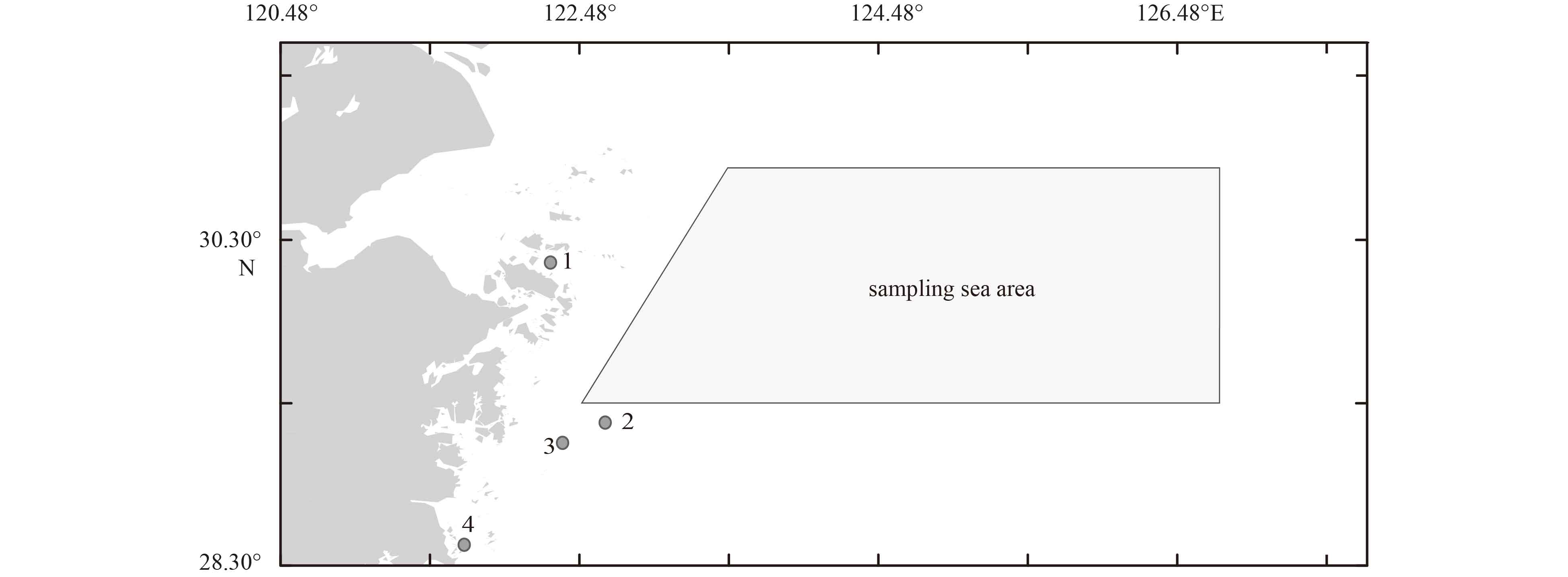
The experimental sample of P. trituberculatus was obtained from May 2015 to May 2016 in the northern East China Sea (29.30°–30.50°N, 122.48°–126.75°E), except when closed fishing season (Fig. 1). P. trituberculatus samples (the seas area in Fig. 1 is the area where the commercial fishing vessel operates, and the individuals of P. trituberculatus were randomly sampled from these vessels) were obtained twice each month, and the sampling fishing gear included crab cages, gillnets, and a single otter trawl. A total of 769 P. trituberculatus individuals were collected. The carapace width (CW, mm), carapace length (CL, mm) and body weight (W, g) of each crab were measured. The samples were grouped according to the CL, and the average weight and proportion of the different size P. trituberculatus were measured to determine the structural composition of the P. trituberculatus in the survey area. Therefore, P. trituberculatus with CW ranging from 60 mm to 80 mm were defined as the recruitment group (Sun et al., 2018).
Figure
1.
Map of sampling area of P. trituberculatus during 2015 and 2016. The points represent the enhancement and releasing areas centered on Zhoushan (1), Ningbo (2), Taizhou (3), and Wenzhou (4).
The abundance of P. trituberculatus during these years are calculated based on the catch data by using Eqs (A1) and (A2). A detailed description of the parameters is given in the Appendix A.
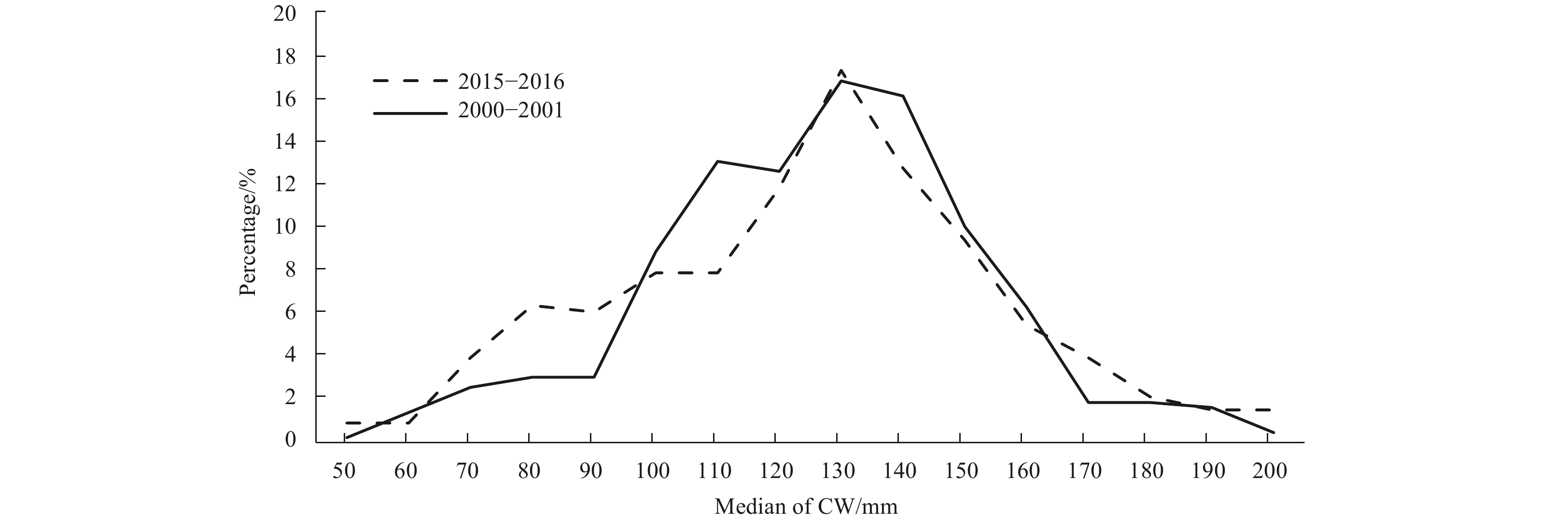
The parameters of natural and fishing mortality come from the studies of Wang et al. (2017a). The comparison of the CW composition to the catch of P. trituberculatus was made in the study sea (Fig. 2), which is not significantly different (P=1). The CW composition in 2015–2016 came from the sample, and the 2000–2001 came from Song et al. (2012). Therefore, the assumption of CW composition to P. trituberculatus in this study are not significantly changed. And spawning stock and recruitment for each year are estimated based on the proportion information obtained from a survey of P. trituberculatus during 2015 and 2016. Recruitment values from 2001 to 2014 are calculated according to the catch and proportions of CW frequencies measured in the survey samples in these two years.
Figure
2.
The CW composition of the catch of P. trituberculatus in the northern East China Sea during 2000–2001 and 2015–2016.
P. trituberculatus is a species released in the study areas for stock enhancement. The annual quantity of releasing crab from the fisheries administration department were obtained. Then, according to the coefficients of natural mortality during the early life history, the abundance of P. trituberculatus resources that survived to the fishing stage was estimated based on the formula of Appendix A. Before 2010, the releasing quantity of P. trituberculatus in the northern East China Sea area is relatively small, and the data are not available. Therefore, on the basis of releasing quantity in 2011, the assumption number of releasing crab in the following year is 10% higher than that of the previous year, and then push forward in turn to obtain the estimated annual release (private communication with fishery managers). Equation (A1) is used to calculate the subsequent abundance coming from the releasing stock when the releasing stock reaches the recruitment specification. Taking into account the large scale releasing activities (the releasing of P. trituberculatus are implemented in most areas of Zhejiang Province, especially in Zhoushan, Ningbo, Taizhou, and Wenzhou), it has a greater impact on the natural population of P. trituberculatus (Fig. 1). Therefore, the biomass coming from the releasing is removed (spawning stock and recruitment) from the fishery statistical data.
2.1.2
Environmental factors
The abundance of fishery resources generally involves a dynamic process. The main factors affecting this process include population number, fishing activities and changes to the marine environment (Sakuramoto, 2005). Considering the effect of environmental variables on the recruitment of P. trituberculatus, the selection of the following main environmental factors: area of red tide (AORT), El Niño index (EINI), sea level height (SLH), sea surface salinity (SSS), typhoon landing times (TYP), and sea surface temperature (SST) in the study area. Among them, the environmental factors which had significant influence on the recruitment of P. trituberculatus were screened out, and the effects of insignificant factors were deleted.
In order to select the environmental factors that have significant effects on the recruitment, the environmental factors have been screened. First of all, the GLM function in R (version 3.5.3) was used to analyze the relevant environmental and biological data from 2001 to 2014, and the regression equation including parent quantity and all environmental independent variables was established. Then the stepwise regression analysis method was used to subtract the environmental factor with small contribution rate and no significance (the selection criterion is Akaike information criterion (AIC)). The environmental factors were continuously subtracted until the value of the environmental factor AIC was no longer reduced. Finally, the remaining independent variables were evaluated, and the effects of the remaining environmental variables on the recruitment are significant (P<0.05). Pearson correlation analysis of the selected environmental factors and the recruitment of P. trituberculatus were made. Histogram and correlation ellipses were also used to analyze the correlation between environmental factors and recruitment. Meanwhile, in order to avoid multicollinearity, the Pearson’s correlation coefficient analysis on environmental variables was used before adding to the Ricker model. The environmental data of SLH and SSS are obtained from http://www.cpc.ncep.noaa.gov, and AORT data are obtained from the China Ocean Yearbook. The monthly data of TYP are obtained from http://tcdata.typhoon.org.cn/dlrdqx_zl.html.
2.2
Analysis methods
2.2.1
S-R model
Between the two traditional S-R relationships, namely, the Ricker and Boverton-Holt models, the former is more sensitive to environmental influences (Zhao et al., 2003). Therefore, the Ricker model is chosen as the basis for analysing the S-R relationship in the current study (Appendix B).
2.2.2
Model-selection criteria
To evaluate the candidate models and select the best one, the model-selection approach based on the principle of parsimony in which several competing hypotheses (candidate models) are adopted and simultaneously confronted with data (Hobbs and Hilborn, 2006; Johnson and Omland, 2004). The AIC and the Bayesian information criterion (BIC) are valid for selecting the most suitable S-R relationships (Wang et al., 2005). The optimal S-R relationship model in this paper is selected according to AIC and BIC standards (Appendix B).
The residual versus fitted, normal quantile-quantile (Q-Q), scale–location and residual versus leverage relationships are used to analyse the two Ricker-type models with environmental factors. The values of recruitment predicted by the above models from 2001 to 2014 are compared with the observed values, and the fitting degree is used as the standard to select the most suitable model reflecting the S-R relationship of P. trituberculatus in the study area.
2.2.3
Model validation
S-R data of P. trituberculatus in the study area from 2015 to 2017 are used to validate the Ricker-type S-R models by comparing the estimated recruitment with the observed recruitment, and then verify the accuracy of the most suitable model.
3.
Results
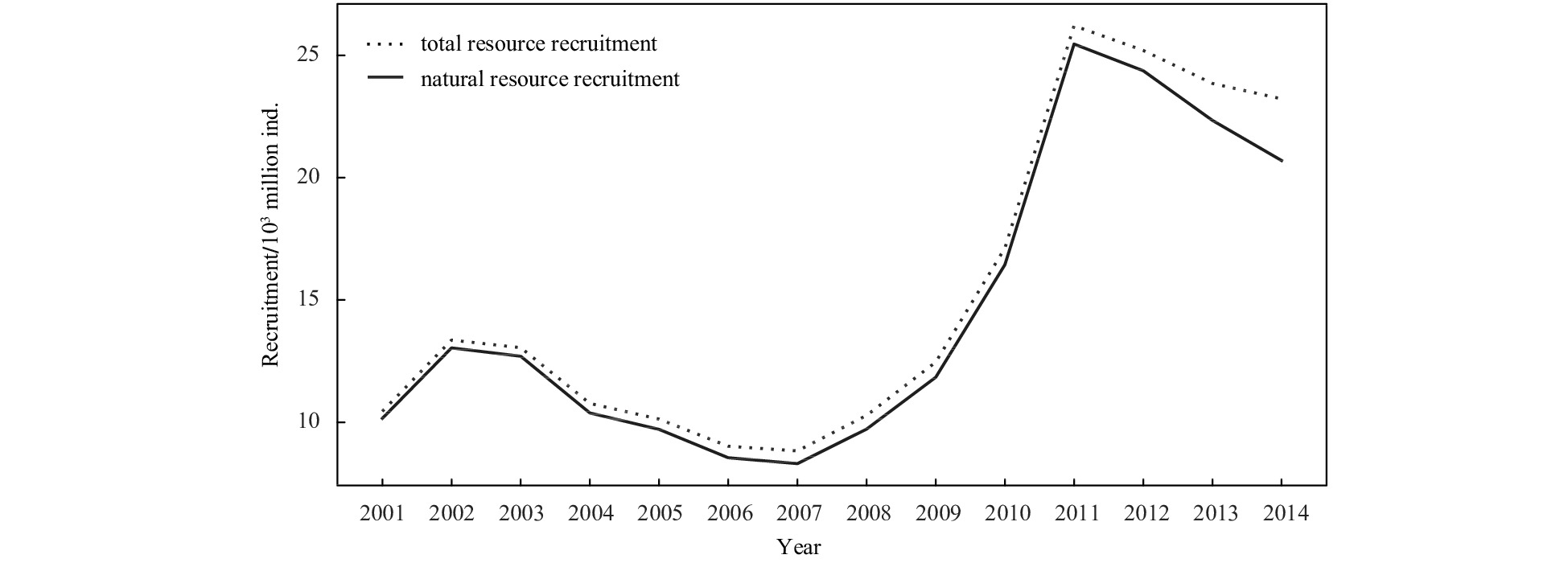
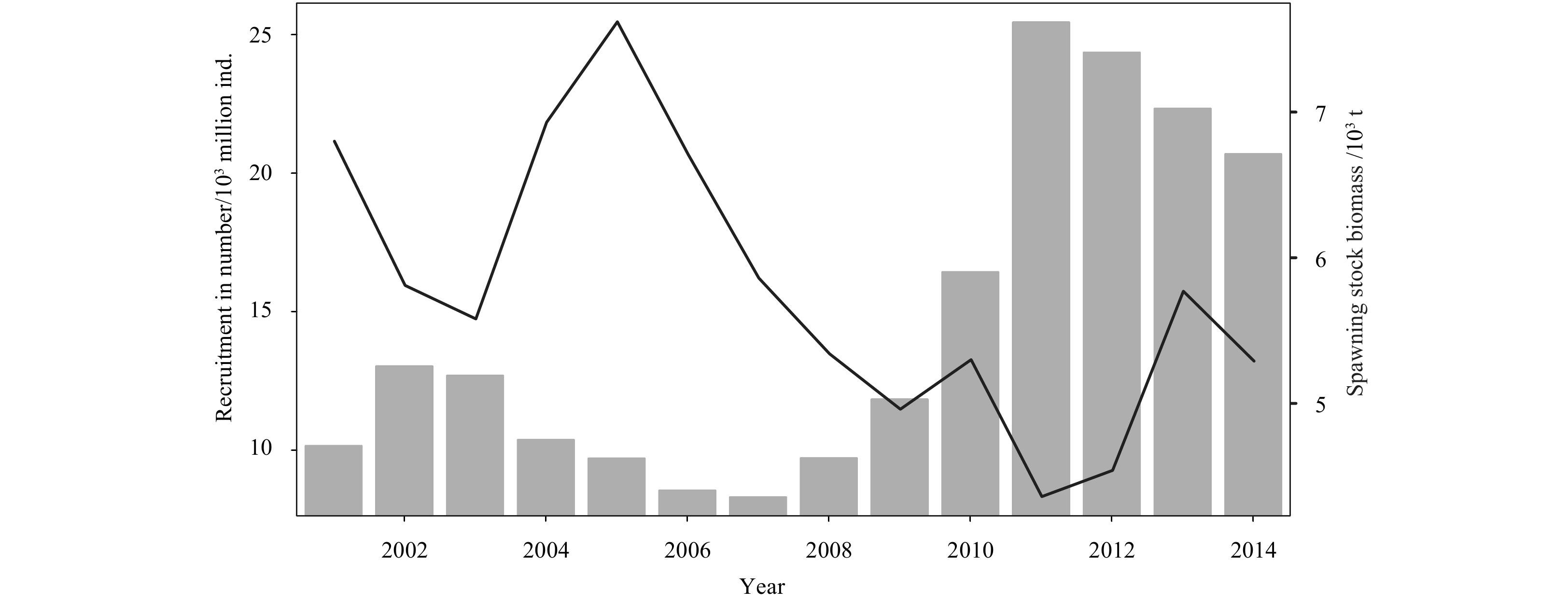
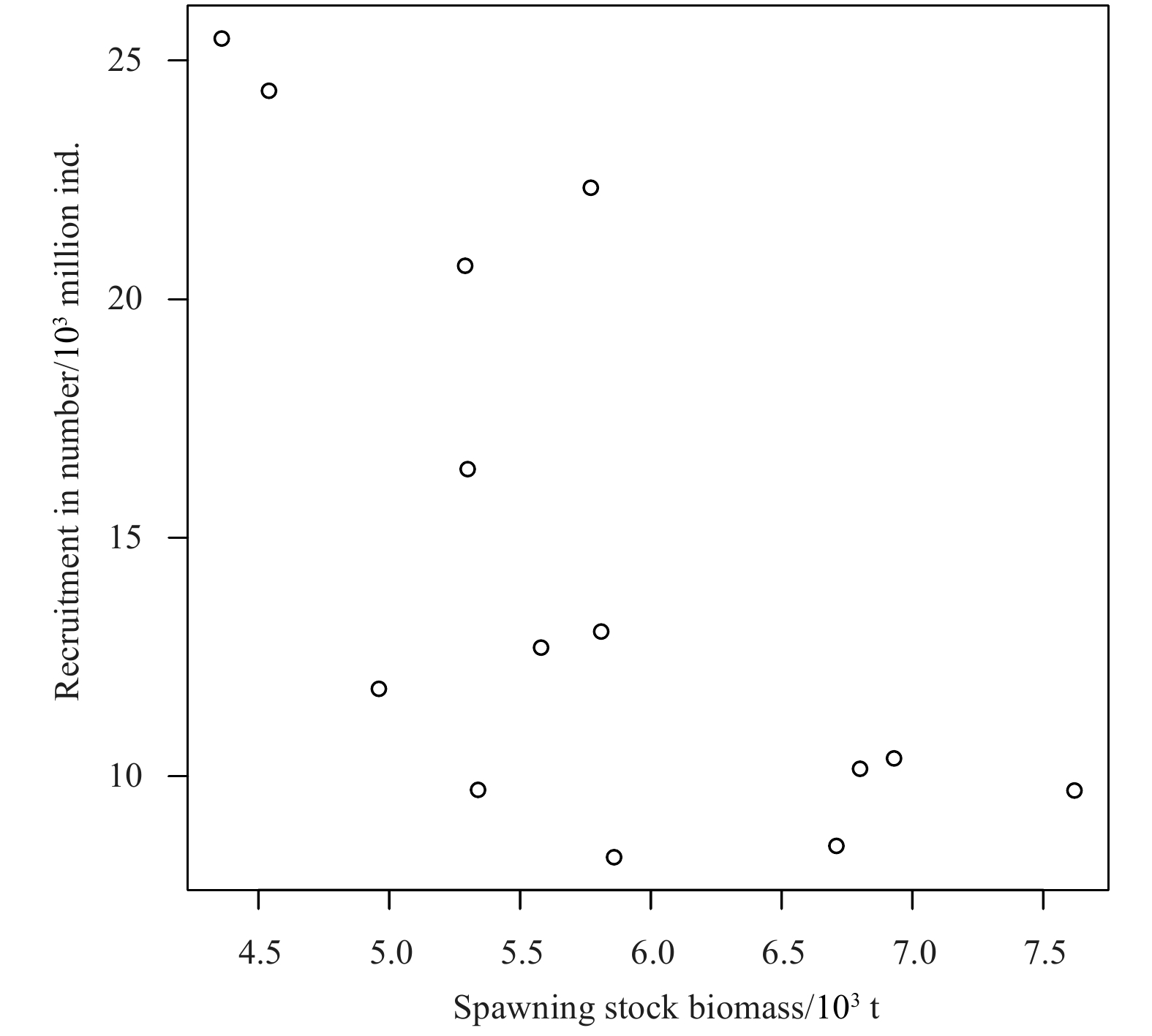
Figure 3 shows that the fit between the total recruitment and recruitment obtained from the natural resources of P. trituberculatus in the period of 2001–2014 is very high. This finding indicates that variations in recruitment are less affected by stock enhancement. The annual variation of spawning stock and recruitment shows that recruitment decreases with increasing spawning stock (Fig. 4). Hence, spawning stock and recruitment were negatively correlated from 2001 to 2014.
Figure
3.
The comparison of the natural resource recruitment and total resource recruitment during 2001–2014.
The results of the gradual screening of environmental factors (Table 1) showed that the SST and EINI are excluded from environmental factors. Simultaneously, the remaining environmental factors are significant difference (P<0.05) (Table 2), and the AORT, SLH, SSS and TYP are selected as the final study variables.
Table
1.
Stepwise regression process of environmental variable selection
One-step model
Degree of freedom
Deviance
AIC
Initial value
−
−
−3.754
-SST
1
0.196
−3.996
-EINI
1
0.206
−5.307
-AORT
1
0.356
0.313
-TYP
1
0.410
2.300
-SLH
1
0.435
3.117
-SSS
1
0.481
4.529
-S
1
0.576
7.061
Note: SST indicates sea surface temperature, EINI indicates El Niño index, AORT indicates red tide area, TYP indicates typhoon landing times, SLH indicates sea level height, SSS indicates sea surface salinity, S indicates spawning stock biomass. The initial value represents the AIC value for all variables. The symbol “–” (the hyphen) in the first column represents the elimination of variables one by one in the regression process.
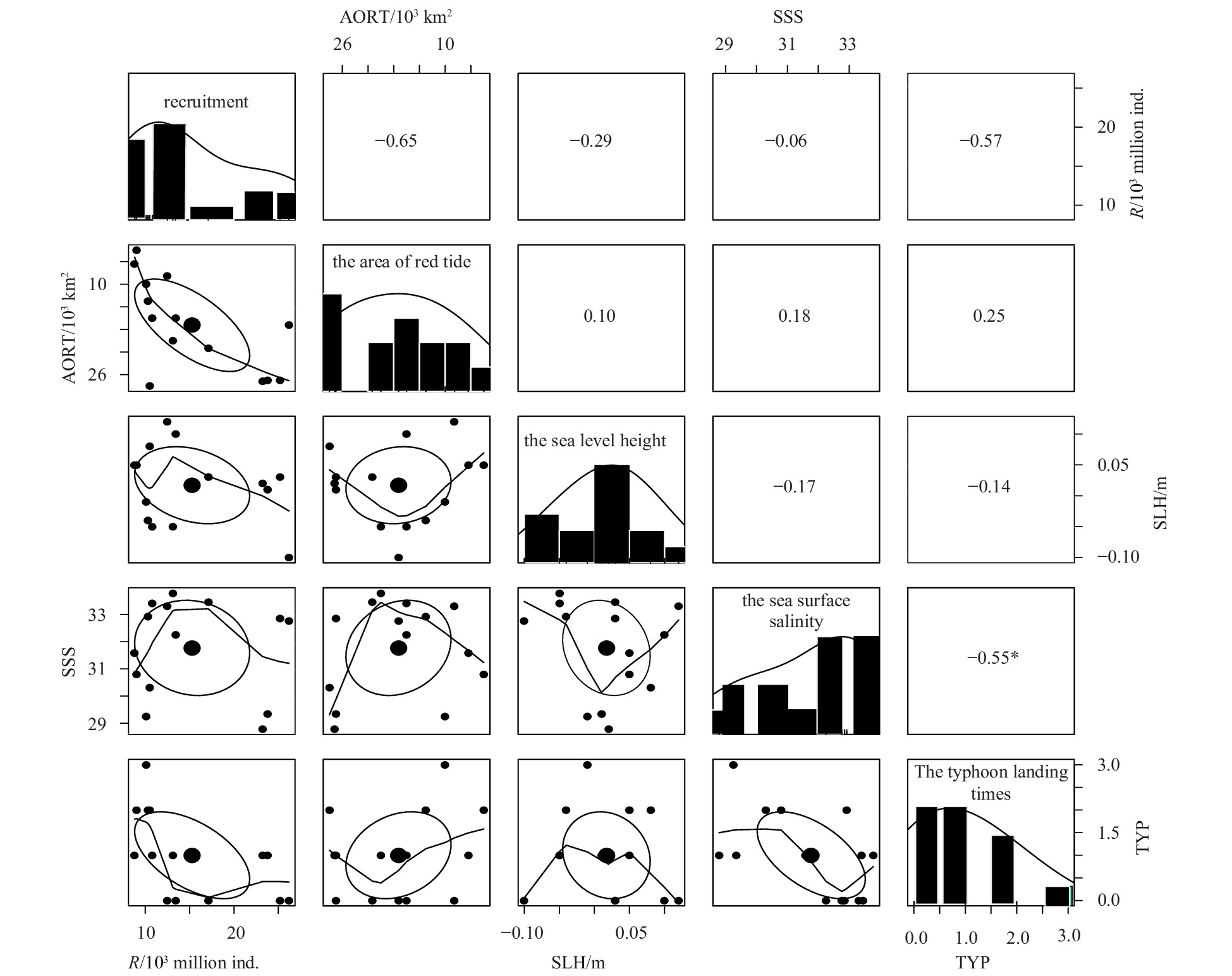
In addition, the correlation analysis of the selected environmental factors showed that the correlation between SSS and TYP was less than 5%. The histogram in Fig. 5 displays the distribution of each environmental factor. In Fig. 5, the elliptical graphics in each scatter plot are called correlation ellipses, and the big solid point represents the center of each ellipse. The correlation between the two variables is represented by the shape of the ellipse. The longer the ellipse is stretched, the stronger the correlation is. Conversely, the closer the shape of an ellipse is to a circle, the weaker the correlation between the two variables are. The curves plotted in the scatter diagrams are described as “loess smooth”, which represents general relationships between changes in the X- and Y-axis. Figure 5, for example, shows that the relative ellipses of Rt+1 and AORT are stretched, which indicates a strong correlation between two variables. This finding is confirmed by the large symmetric correlation coefficient (−0.65) obtained. In addition, the curves of Rt+1 and AORT show that recruitment decreases with increasing AORT.
Figure
5.
Pearson’s correlation coefficient and screening results of environmental variables in the northern East China Sea from 2001 to 2014. Recruitment means Rt+1, where Rt+1 refers to the recruits in the year t+1; *means significant at a significance level of 5%, P value=0.04; and the numbers surrounding the figure are the variable values of the 5×5 matrix, which represent the numerical range of each variable.
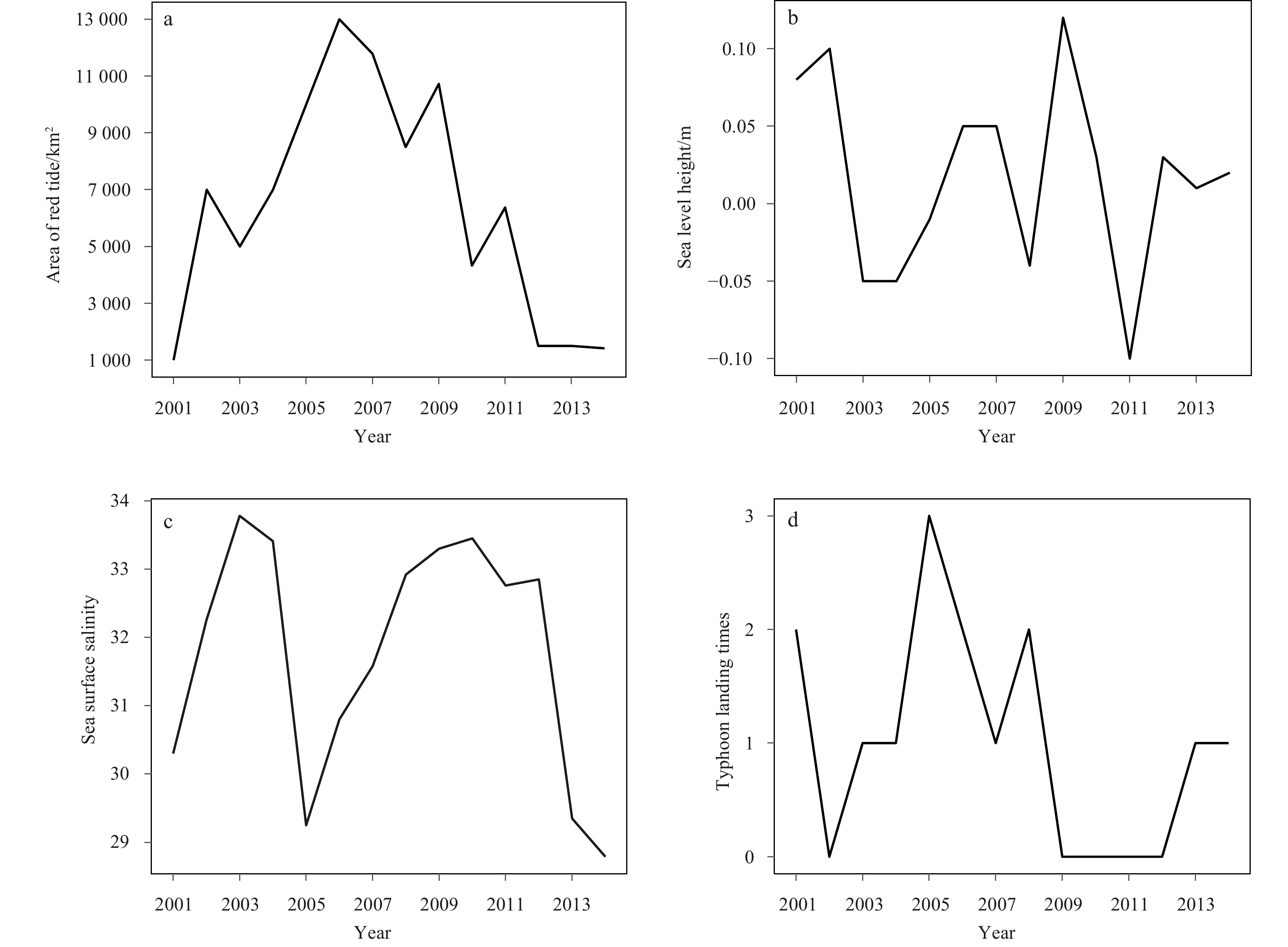
Figure 6 shows the variations of the four environmental factors from 2001 to 2014. The AORT in the study area increased sharply from 1 000 km2 to 13 000 km2 from 2001 to 2006 (Fig. 6a). After 2006, AORT decreased gradually to approximately 1 420 km2, although two turning points could be observed. Figure 6b shows an up/down variation of SLH from −0.05 m to 0.05 m. The highest and lowest SLH in 2009 and 2011were 0.12 m and −0.1 m, respectively. Figure 6c shows the change of SSS, which first increased and then decreased during 2001–2005. SSS dropped to 29.25 in 2005 and rose every year prior to 2010. After 2010, SSS continuously decreased to a minimum of 28.79 in 2014. Figure 6d shows the variation of TYP, which reveals a maximum value of 3 in 2005. Except in 2002 and 2009–2012, all TYP values were between 1 and 2.
Figure
6.
The variation of environmental factors with time. a. The year trend of the area of red tide; b. the year trend of the sea level height; c. the year trend of sea surface salinity; d. the year trend of typhoon landing times in the northern East China Sea from 2001 to 2014.
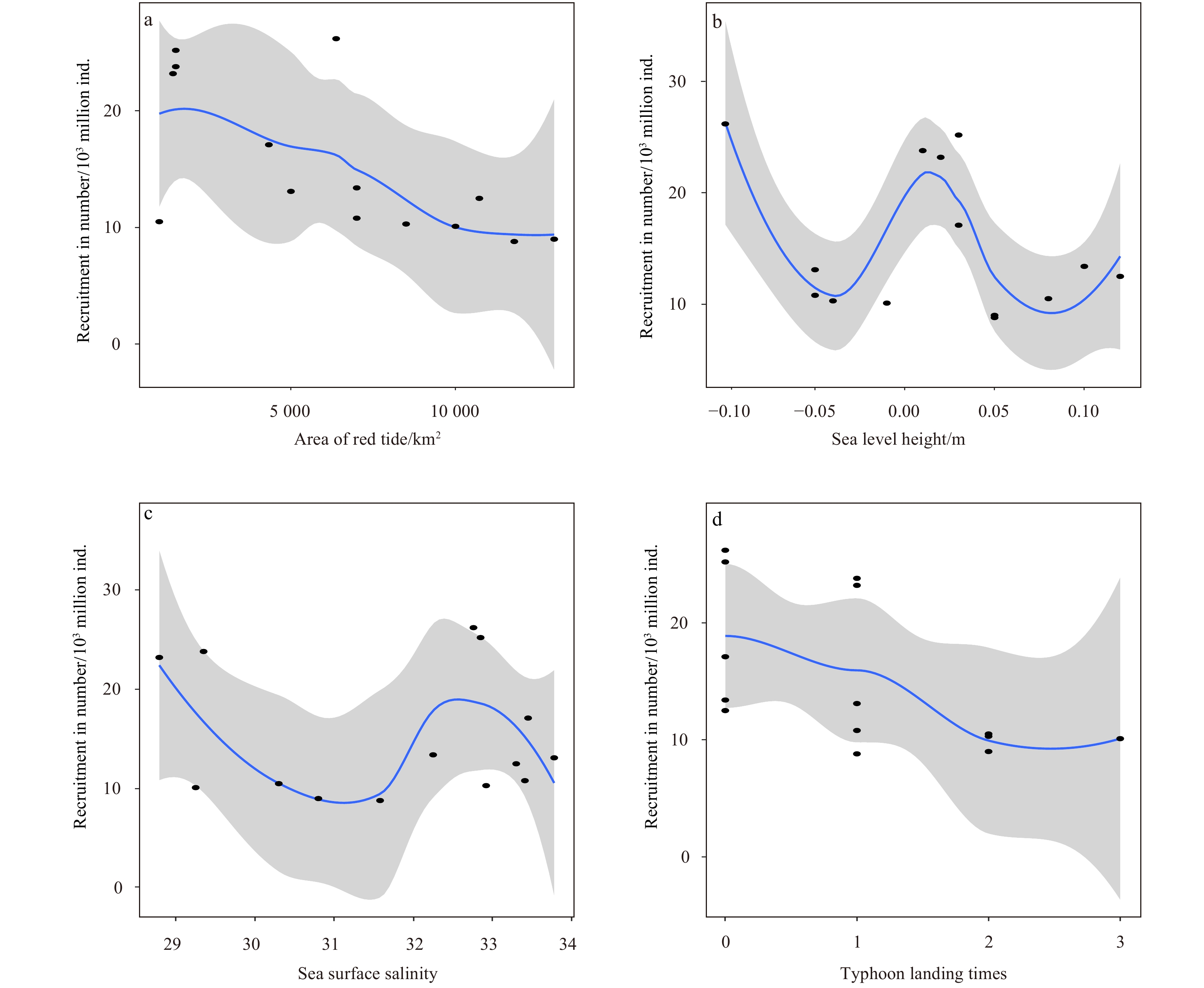
By comparing the changes of environmental factors and recruitments of P. trituberculatus with years, the results showed the recruitment varied greatly in the year when the environmental factors changed greatly. Recruitment of P. trituberculatus decreased with the increase of AORT and had a negative correlation with AORT (Fig. 7a). Moreover, in Fig. 7b that the effect of sea level height on the recruitment of P. trituberculatus is complex. When the SLH was between −0.10 m and −0.05 m, the recruitment of P. trituberculatus was reduced. When the SLH was between 0.01 m and 0.075 m, the recruitment of P. trituberculatus also decreased with the increase of SLH. However, when the SLH changed from −0.05 m to 0.01 m, the recruitment of P. trituberculatus increased with the increase of the SLH. Figure 7c shows the relationship between SSS and changes in the recruitment of P. trituberculatus. When SSS was approximately 28.5, the maximum recruitment was approximately 23 billion individuals. The recruitment of P. trituberculatus decreased with increasing salinity, until approximately 31.5, beyond which recruitment increased sharply with continuous increases in salinity. When SSS>32.5, recruitment decreased once more. In Fig. 7d there is a clear trend that the recruitment of P. trituberculatus decreased with the increase of TYP.
Figure
7.
Change trend of the influence of environmental factors on R of P. trituberculatus. The gray area indicating the 95% confidence interval.
Overall, the Ricker model with environmental factors has an advantage over the traditional Ricker model. Figure 8 indicates that the S-R relationship does not present the trend of the traditional Ricker curve. Comparing the two Ricker-type models with environmental factors with the traditional Ricker model is showed, that the AIC and BIC of the traditional Ricker model are 10.513 and 12.430 (Table 3), which are greater than those of the two Ricker-type models with environmental factors (Tables 4 and 5). This finding suggests that environmental factors have a significant effect on the recruitment of P. trituberculatus. Different quantities of environmental factors are added to the Ricker model as the two kinds of candidate environment-based Ricker models, and find that the smallest AIC and BIC values appear in the models with four environmental factors. While the fit relationship between the model incorporating one environmental factor and S-R is the worst, with AIC and BIC of 3.186 3 and 5.742 5, respectively. For the Ricker-type 2 model, when adding four environmental factors, the AIC and BIC values are −5.307 2 and −0.833 8, respectively, which are the minimum values of the Ricker-type 2 candidate model (Table 4). Similarly, when the different quantity of environmental factors are added to the Ricker-type 3 model, different results are obtained, and the minimum AIC and BIC appear in the model with four environmental factors, whose values equal to −1.811 and 2.023, respectively (Table 5). Therefore, the model with four environmental factors in Ricker-type 2 is considered to be the optimal model since its AIC and BIC values are smaller. The specific forms of Model 2 (the optimal model in Ricker-type 2) and Model 3 (the optimal model in Ricker-type 3) can be expressed as follows:
Figure
8.
Scatter plot of spawning stock biomass and recruitment of P. trituberculatus during 2001–2014.
Table
4.
Comparison of the significant test results of the Ricker-type 2 (an environment-based Ricker model in which with log-linear environmental impact) with different quantity of environmental factors for Portunus trituberculatus in the northern East China Sea
NEF
Environmental factor
Coefficients
Estimate
Std. error
t value
P value
1
AORT
Intercept
3.490 04
0.395 57
8.823
2.55×10⁻⁶***
Coefficients of S
−0.397 71
0.070 35
−5.653
0.000 148***
Coefficients of AORT
−0.052 31
0.016 21
−3.227
0.008 055**
AIC
3.186 3
BIC
5.742 5
2
AORT, SLH
Intercept
3.471 59
0.393 99
8.811
5×10⁻⁶***
S
−0.392 72
0.070 16
−5.597
0.000 228***
AORT
−0.051 05
0.016 17
−3.156
0.010 224*
SLH
−1.077 83
1.022 99
−1.054
0.316 858
AIC
3.712 5
BIC
6.907 8
3
AORT, SLH, SSS
Intercept
5.819 77
1.534 47
3.793
0.004 265**
S
−0.454 42
0.076 28
−5.957
0.000 213***
AORT
−0.041 73
0.016 21
−2.574
0.029 975*
SLH
−1.366 05
0.971 95
−1.405
0.193 448
SSS
−0.064 40
0.040 86
−1.576
0.149 434
AIC
2.299 8
BIC
6.134 1
4
AORT, SLH, SSS, TYP
Intercept
6.841 21
1.210 75
5.650
0.000 481***
Coefficients of S
−0.300 44
0.079 38
−3.785
0.005 351**
Coefficients of AORT
−0.030 80
0.012 80
−2.406
0.042 794*
Coefficients of SLH
−2.469 03
0.830 23
−2.974
0.017 765*
Coefficients of SSS
−0.118 02
0.036 19
−3.261
0.011 515*
Coefficients of TYP
−0.258 27
0.091 95
−2.809
0.022 885*
AIC
−5.307 2
BIC
−0.833 8
Note: NEF represents the quantity of environmental factors that are added to the model. “*”is the significance code, “***” means P value ∈ [0, 0.001], “**” means P value ∈ (0.001, 0.01], “*” means P value ∈ (0.01, 0.05], “.” means P value ∈ (0.05, 0.1], no code means P value ∈ (0.1, 1). Generally, the P value less than 0.05 (typically ≤0.05) means statistically significant.
Table
5.
Comparison of the significant test results of the Ricker-type 3 (an environment-based Ricker model in which with ln-quadratic polynomial environmental impact) with different quantity of environmental factors for Portunus trituberculatus in the northern East China Sea
NEF
Environmental factor
Coefficients
Estimate
Std. error
t value
P value
1
AORT
Intercept
3.641 02
0.426 90
8.529
3.54×10⁻⁶***
Coefficients of S
−0.423 51
0.073 82
−5.737
0.000 131***
Coefficients of ln(AORT)
−0.214 87
0.078 03
− 2.754
0.018 769*
AIC
5.173
BIC
7.729
2
AORT, SSS
Intercept
9.494 91
1.724 19
5.507
0.000 184***
Coefficients of S
−0.443 71
0.064 57
−6.872
2.68×10⁻⁵***
Coefficients of ln(AORT+SSS)
−1.671 12
0.470 43
−3.552
0.004 533**
AIC
1.814 8
BIC
4.371 1
3
AORT, SSS, SLH
Intercept
8.210 82
2.028 39
4.048
0.002 33**
Coefficients of S
−0.471 68
0.068 03
−6.933
4.03×10⁻⁵***
Coefficients of ln(AORT+SSS)
−1.365 81
0.533 14
−2.562
0.028 28*
Coefficients of ln(SLH2)
−0.052 80
0.045 61
−1.158
0.273 96
AIC
2.054 5
BIC
5.249 8
4
AORT, SSS, SLH, TYP
Intercept
7.445 20
1.769 73
4.207
0.002 28**
Coefficients of S
−0.339 89
0.084 21
−4.036
0.002 95**
Coefficients of ln(AORT+SSS)
−1.353 87
0.455 80
−2.970
0.015 69*
Coefficients of ln(SLH2)
−0.079 82
0.040 94
−1.949
0.083 04 .
Coefficients of (TYP+1)
−0.362 84
0.167 66
−2.164
0.058 67 .
AIC
−1.811
BIC
2.023
Note: NEF represents the quantity of environmental factors that are added to the model. “*”is the significance code, “***” means P value ∈ [0, 0.001], “**” means P value ∈ (0.001, 0.01], “*” means P value ∈ (0.01, 0.05], “.” means P value ∈ (0.05, 0.1], no code means P value ∈ (0.1, 1). Generally, the P value less than 0.05 (typically ≤0.05) means statistically significant.
The selected SLHs is notably negative in some years. The square of SLH is used to avoid the problem of negative numbers, which are not logarithmic (Campbell, 2004).
3.4
Model validation
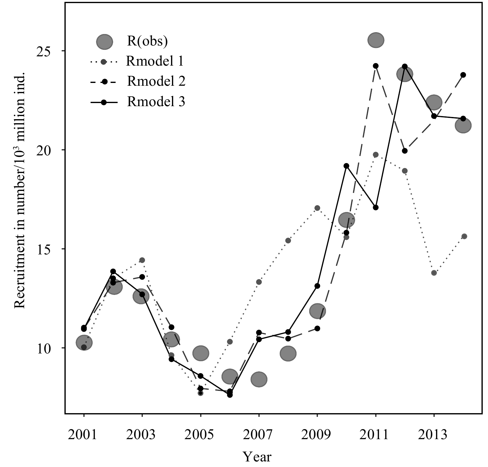
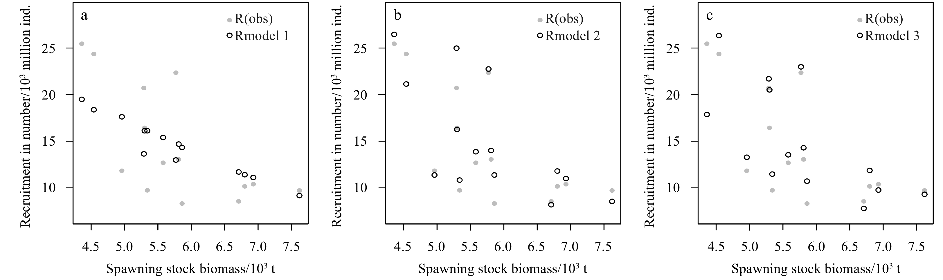
The fitted diagnostic results of Model 2 and Model 3 are shown in Fig. 9. From the Figs 9a and e, the residual and estimated values were irrelevant. In addition, the normal Q-Q plots (Figs 9b and f) of the two models indicate that the residuals of the models have normal distributions. In this regard, slight differences are observed amongst the models. The scale-location results (Figs 9c and g) show that the residuals in Models 2 are randomly distributed (the more random the distribution, the better the model). The values of 0.5 and 1 in the residuals and leverage curves are usually used as criteria for judging outliers. By comparing the results of Model 2 (Fig. 9d) and Model 3 (Fig. 9h), there is an outlier in the lower right corner of Fig. 9h, whose value is greater than 0.5. The research indicate that data points with large residuals (outliers) or high leverage can distort the outcome and accuracy of a regression (Kim et al., 2001). In other words, this outlier greatly contributes to the deviation of the model from the actual situation. In this case, if the abnormal points are removed, the model parameters will change greatly, which indicates that the model is not regarded as sufficiently. Thus, Model 3 does not comply with the criteria for the optimal model. Recruitment values during 2001–2014 are predicted using the established models (including the Ricker model, Model 2 and Model 3) and fitted to the observed Rt+1 (Figs 10 and 11). Results show that Model 2 fits Rt+1 better than Model 3, which is consistent with the results of AIC and BIC model selection. In summary, the model validation results show that Model 2 is more reasonable than Model 3 for describing the effects of environmental factors on S-R relationship.
Figure
9.
Fitted diagnostic diagram of Ricker-type S-R model. Figures 9a–d represent the result of Model 2 (Ricker model with ln-linear environmental impact (Ricker-type 2)) and Figs 9e–h represent the result Model 3 (Ricker model with ln-quadratic polynomial environmental impact (Ricker-type 3)): Figures 9a and e are the residual vs. fitted values, Figs 9b and f are the normal Q-Q plots, Figs 9c and g are the scale-location results, Figs 9d and h are the residuals vs. leverage. The solid line indicates the trend of the Y-axis changing with the X-axis, the dotted line indicates the criteria for judging outliers.
Figure
10.
Comparison of different Ricker models from 2001 to 2014. R(obs) is the observed recruitment value, Rmodel 1, Rmodel 2 and Rmodel 3 are the predicted value of Model 1 (traditional Ricker model), Model 2 (an optimal model in Ricker-type 2 model with ln-linear environmental impact), Model 3 (an optimal model in Ricker-type 3 model with ln-quadratic polynomial environmental impact), respectively.
Figure
11.
Comparison of different S-R model fitting. R (obs) is the observed recruitment value, Rmodel 1 (a) is the predicted values of the traditional Ricker model. Rmodel 2 (b), Rmodel 3 (c) are the predicted values of Ricker-type 2 model (an optimal model in Ricker-type 2 model with ln-linear environmental impact) and Ricker-type 3 model (an optimal model in Ricker-type 3 model with ln-quadratic polynomial environmental impact), respectively.
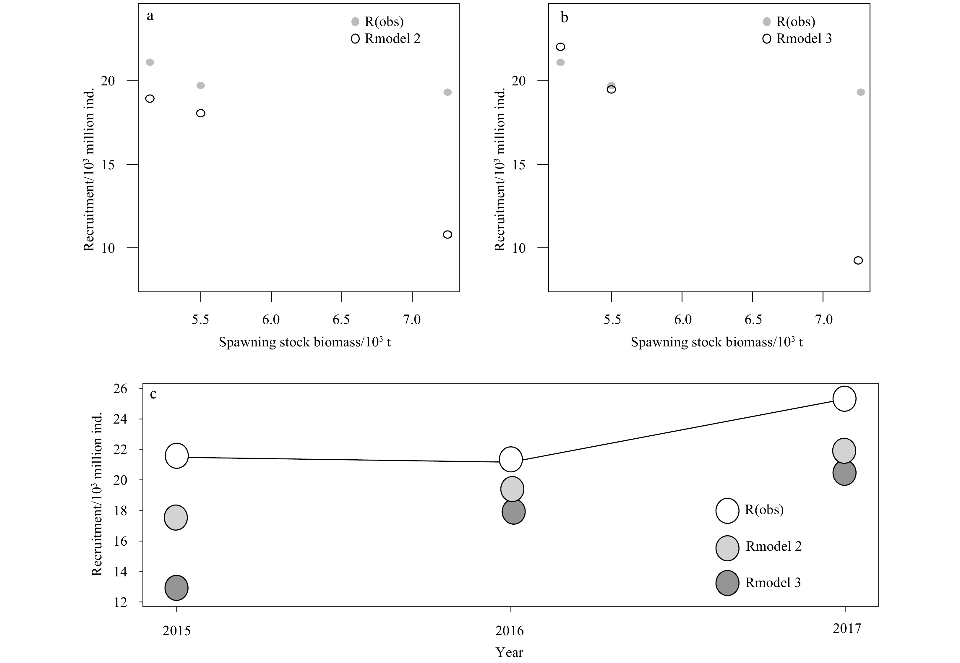
The predicted recruitment values for 2015–2017 using two Ricker-type models, Model 2 and Model 3 are compared with the observed values. The prediction results of Model 2 are closer to the observed values than Model 3 (Fig. 12).
Figure
12.
Comparison of Ricker-type model predictions for 2015–2017. Rmodel 2, Rmodel 3 represent the recruitment values predictions for Model 2 (an optimal model in Ricker-type 2 model with ln-linear environmental impact), Model 3 (an optimal model in Ricker-type 3 model with ln-quadratic polynomial environmental impact), respectively, and R (obs) is the observed recruitment value. The figure shows the comparison of the predicted and observed values of the two Ricker-type models (a, b), and the comprehensive comparison of the two models (c).
In this study, the effects of four environmental factors on the S-R relationships in the northern East China Sea were analysed. It is indicated that the effects of these four environmental factors on the recruitment of P. trituberculatus are significant. They can be divided into two categories: (1) AORT and TYP, which cause continuous decreases in the recruitment of P. trituberculatus, and (2) SLH and SSS, which lead to fluctuations in the recruitment of P. trituberculatus. Assume that TYP and AORT can directly destroy the living environment of marine organisms by disrupting their feeding base and affecting their distribution. Hence, the recruitment of P. trituberculatus will continuously decline under these factors.
Red tide is an important marine disaster. It destroys the marine ecological balance, endangers marine fisheries and aquatic resources and even threatens human health (Kirkpatrick et al., 2004). Red tide can cause death in various marine species, including fish (Neely and Campbell, 2006; Wang et al., 2001; Flaherty and Landsberg, 2011), shellfish and benthic organisms (Arzul et al., 1994). Rashed-Un-Nabi et al. (2010) found that the biomass of phytoplankton in seawater is generally high and that large diurnal variations of dissolved oxygen and pH occur after a red tide bloom. Moreover, anaerobic environments, which threaten the survival of various organisms, easily develop at the bottom of the water column. Considering that the red tide season occurs simultaneously with the spawning season of P. trituberculatus in the northern East Chinese seas (Lou et al., 2006), the newly hatched larvae have poor viability, which will lead to a decrease in recruitment. Amongst other Chinese seas, the occurrence and area of red tide are largest in the East China Sea (Zhu et al., 2009). Therefore, AORT is a significant factor affecting the recruitment of P. trituberculatus.
Several studies have indicated that important economic fish, shrimp, crab, and shellfish disappear as the sea level rises (Paulay, 1990; Schaaf, 1996; Fulford et al., 2014). Increases in SLH result in extreme events, such as tsunamis and storm surges, and bring about large losses in fishery resources (Costa et al., 1994; Jiao et al., 2015). Changes in SLH also damage the habitat of many organisms. The habitat of P. trituberculatus is mainly concentrated in shallow water; such waters are highly susceptible to sea-level changes, which causes significant changes in the recruitment of the species. In spring and summer, P. trituberculatus lays eggs and grows in shallow sea areas approximately 3–5 m from the shore, especially in estuaries. The crabs then migrate to offshore areas of approximately 10–30 m in autumn and winter to overwinter. Increases in SLH have an important effect on the success rate of spawning and survival rate of early juvenile crabs, which make up an important recruitment group. But juvenile crabs are less able to resist and adapt to risks than adult crabs. This study indicates that the recruitment of P. trituberculatus decreases when SLH is between −0.10 m and −0.05 m or between 0.01 m and 0.075 m due to the destruction of their habitat and increased risk of wave attack or storm surges. Therefore, the changes in SLH may have a direct effect on the recruitment of P. trituberculatus.
Salinity is a major environmental factor affecting the survival and development rate of crustacean larvae (Teal, 1958; Giménez, 2003; Baylon and Suzuki, 2007). Salinity can also affect the distribution of crustacean (Hall and Burns, 2003). In a study on suitable salinity levels for the growth of P. trituberculatus zoeae, Zhang and Li (1992) find that the crabs are inclined to grow in the sea of their spawning stocks and that their survival rate is severely reduced if they deviate from the range of salinity appropriate for spawning colonies. High salinity (above 35) could inhibit the hardening of the shell of P. trituberculatus zoeae, thereby causing mass mortality (Lu et al., 2012). It is reported that when the salinity of the cultured water body is controlled at about 25, it will be more beneficial to the molting, synchronization, and growth of P. trituberculatus. Romano and Zeng (2006) studied the effects of high salt environments on the growth and development of P. trituberculatus and concluded that the food intake of P. trituberculatu in this environment would decrease, which could affect its growth rate. Interestingly, the recruitment of P. trituberculatus decreased from 20.7×10³ million individuals to approximately 8.3×10³ million individuals when the salinity is from 29.0 to 31.5. Similar results have been reported by other researchers (Shentu et al., 2015). Thus, the recruitment of P. trituberculatus may be greatly affected when the water salinity exceeds the optimum range.
Typhoon can affect the recruitment of P. trituberculatus, which may led to a decrease of the catch of P. trituberculatus. After the typhoon, the proportion of the catch of crabs in the total catch in the western Guangdong fishing grounds drop from 0.05% to 0.03% (Yu et al., 2015). Considering that a typhoon can rapidly change the water environment within a short time, it inevitably results in physiological and biochemical effects on P. trituberculatus (Wang et al., 2016). Typhoon transit causes a series of stress responses in P. trituberculatus. It can also cause physical dysfunction, body injury and other issues in organisms, resulting in a large number of deaths over a short period of time (Chen et al., 2018). The occurrence of a typhoon is generally accompanied by changes in SST, salinity and seawater nutrients. Fu et al. (2016) investigated the effects of typhoons “Nari” and “Wipha” in 2007 and observed obvious changes in SST and chlorophyll a concentration in the East China Sea; specifically, the SST dramatically dropped. Changes in SST affect the feeding and behavior of P. trituberculatus, causing a decrease in recruitment. The main spawning period of P. trituberculatus in the northern East China Sea occurs from April to July, and the peak period of crab larval growth is from early June to mid-September (Ariyama and Secor, 2010; Ye et al., 2014; Whitehead et al., 2009).
Furthermore, although the results of this study show that the relationships between SST and EINI and the recruitment of P. trituberculatus are not significant, the impact cannot be ignored. It has previously been observed that SST has a significant impact on the catch of P. trituberculatus in the East China Sea, but there is no significant relationship between EINI and catch fluctuation (Yan, 2019). In contrast, Guan and Xuan (2019) reported that both EINI and SST have an impact on the recruitment of P. trituberculatus in the East China Sea. The reason why the above two environmental factors were not significantly related to the recruitment of P. trituberculatus in this study area may be because the SST and recruitment data were using the annual average values, instead of a specific month (August) (Wang et al., 2017b; Yuan et al., 2016) or season (spring spawning season) (Song et al., 2017), which may weaken the influence of SST on recruitment.
4.2
S-R models
In the traditional Ricker model, spawning stock is the only factor affecting the growth of recruitment, which is not suitable for many cases (Zhan, 1995). Cao et al. (2010) find that a model with environmental factors can simulate fluctuations in recruitment over a short period of time. By contrast, the Ricker model without environmental factors can only describe the average trend of recruitment over long periods. Results indicated that the Ricker model with environmental factors can effectively estimate recruitment. The research suggests that the two Ricker-type models considering environmental factors can better describe the S-R relationship than the traditional Ricker model. The natural environment is very complex, but the traditional Ricker model only considers spawning stock as a single factor to predict recruitment, which is inadequate. The growth history of P. trituberculatus is affected by different environmental factors at various stages, which could affect their extent of recruitment. Hence, environmental conditions should be considered when studying the life history of this species because these conditions can play an important role in the growth and development of organisms. Keyl and Wolff (2008) found that variations in fishing stock can be better described if environmental or climatic variability is incorporated into the relevant fishery models, which is consistent with the results on this study. According to the AIC and BIC between Models 2 and Models 3, the model in which all the four environmental factors are added to Ricker-type 2 (ln-linear) presents better results than the Ricker-type 3 (ln-quadratic polynomial).
In the Ricker model, β is an index related to density-dependent mortality, and α is related to density-independent mortality (Zhan, 1995). The effects of environmental factor on the recruitment biomass are usually density-independent, i.e. organisms do not suffer different environmental effects due to different densities. Thus, it is reasonable to add the environmental factors to α. Nevertheless, the relationship between α and environmental factors will affect the performance of S-R relationship. As the research results in this paper show that the multiplicative relationship is better than the additive relationship. Model 2 and Model 3 are not only different in the model structure (ln-linear environmental impact and ln-linear environmental impact, respectively), but also different in the influence mechanism. In the traditional Ricker model, α is a group-independent index. For the Model 3, the environmental factors add to it do not affect the α directly, while for the Model 2, all the environmental factors directly affect the α, which may be consistent with the influence mechanism of the parameter on the recruitment. In the process of adding Model 3 (the additive relationship), it is actually a single environment that individually affects the amount of recruitment. In contrast, the addition of each environmental factor in the process of constructing Model 2 (the multiplicative relationship) will make the final result affected by the parameter α, which is consistent with the influence mechanism of the parameter. In summary, the Model 2 is more reasonable than the Model 3 to describe the effects of environmental factors on S-R.
Cao et al. (2010) showed that changes in environmental factors determine recruitment, that is, the better the environment, the higher the hatching and survival rates of juvenile fish and the higher the recruitment abundance. The fluctuation of resources could be attributed to changes in environmental conditions and numbers of fish parents. Thus, high recruitment is observed when the optimum spawning stock biomass and favorable environmental conditions occur simultaneously (Chen, 2001; Zheng et al., 2008). Many researchers have used simulation methods based on the evaluation of current management policies to study the effects of red tide events on fishery resources, investigate the response to future accidental natural deaths and develop the corresponding fishing strategies (Harford et al., 2018). Thus, the addition of different environmental factors to the Ricker-based model should be suitable for different Ricker-type model and could be very important for improving the fitting accuracy of the S-R model of P. trituberculatus. Considering the effects of environmental factors also contributes to decision-making responses to emergencies or prevention of the reduction of fishing quotas to achieve fishery objectives and management structures.
The results in this paper indicate that environmental factors can give great impact on the S-R relationship of P. trituberculatus, and the position of factors and the number of environmental factors in the Ricker model also have important effects on the S-R relationship of P. trituberculatus. The Ricker-type model with environmental factor can well describe the S-R relationship of P. trituberculatus. Therefore, future effective management and development of the P. trituberculatus ought to take into account the possibility of unexpected events related to climate or the marine environment. Continuously collect and regularly assess the marine environmental data and the fishing data of P. trituberculatus (Ho et al., 2020) is crucial to better understand the relationship between environment and the change of abundance. Simultaneously, it is also important to establish a meteorological warning mechanism to pay attention to the environmental factors and the population dynamics of P. trituberculatus. When P. trituberculatus is affected by environmental factors or the recruitment is not enough to maintain the sustainability of the species, measures such as quota management or stock enhancement should be taken in time.
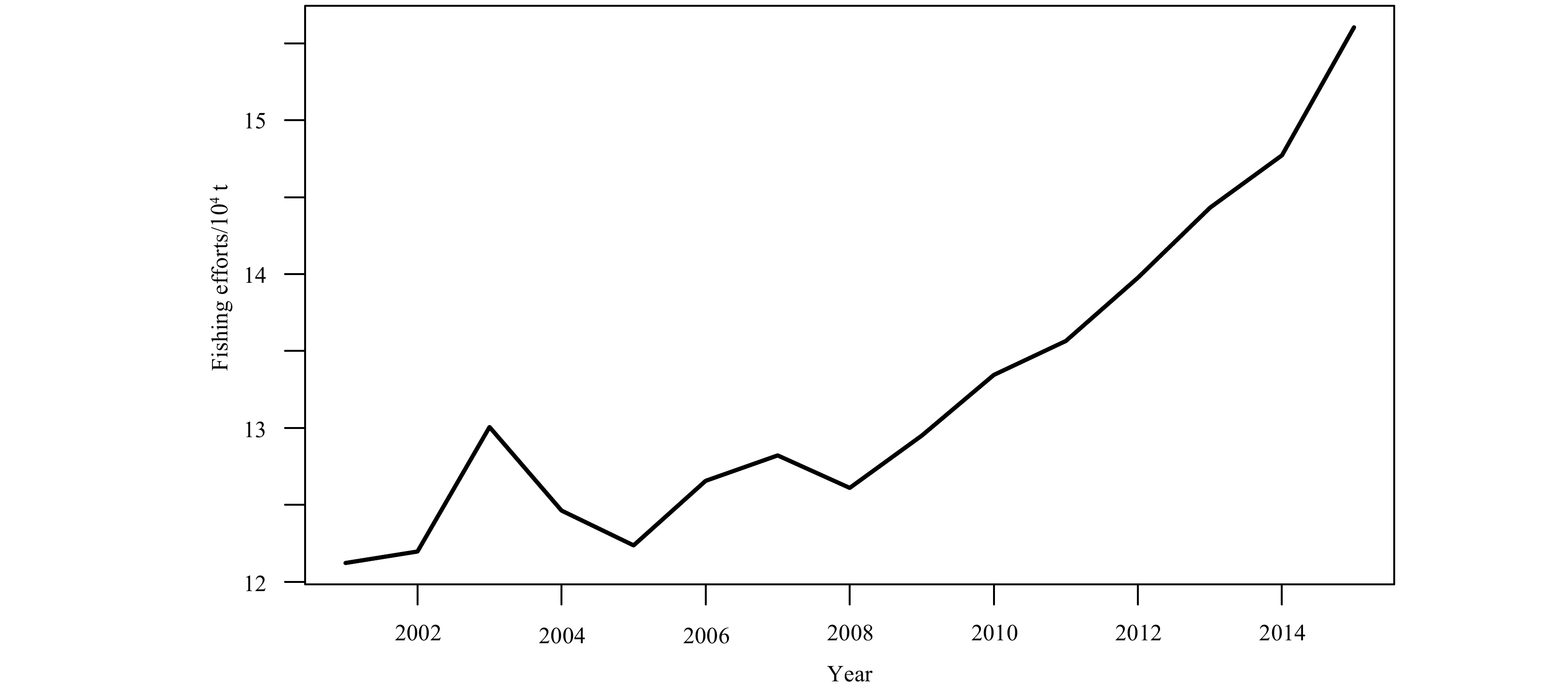
Of course, other factors may also affect recruitment, such as human interference including fishing and releasing. Figure 13 shows the changes of the fishing effort of the P. trituberculatus fishery in the East China Sea from 2001 to 2015. To a certain extent, changes in fishing effort will indirectly affect the size of recruitment by changing the spawning stock. Therefore, it is also important to consider the fishing effort as one impact factor in the future studies for the sustainable development and utilization of P. trituberculatus resources (Fu et al., 2018). It can be seen that the mechanism of the recruitment of P. trituberculatus is complicated. In the future analysis of the S-R relationship of P. trituberculatus, environmental and non-environmental factors should be taken into consideration in order to better evaluate the population dynamics and scientific management of the resource of P. trituberculatus.
Figure
13.
Annual variation of fishing efforts of Portunus trituberculatus in the northern East China Sea during 2001–2015.
In addition, due to the limitations of the data, a small number of environmental factors and short time series are considered in this study. However, the dynamic model established based on the influence of annual environmental change on recruitment has been tested and predicted with good results. This ensures the reliability of the results and has a certain predictability for the supplementation of P. trituberculatus under environmental impact. In future studies, the screening for more environmental factors based on the characteristics of P. trituberculatus growth and development, as well as the living environment is important, so as to establish a more robust S-R model.
Acknowledgements
We gratefully thank the anonymous reviewers for their comments on our draft of this paper.
Anderson C I H, Rodhouse P G. 2001. Life cycles, oceanography and variability: ommastrephid squid in variable oceanographic environments. Fisheries Research, 54(1): 133–143. doi: 10.1016/s0165-7836(01)00378-2
[2]
Ariyama H, Secor D H. 2010. Effect of environmental factors, especially hypoxia and typhoons, on recruitment of the gazami crab Portunus trituberculatus in Osaka Bay, Japan. Fisheries Science, 76(2): 315–324. doi: 10.1007/s12562-009-0198-6
[3]
Arzul G, Gentien P, Crassous M P. 1994. A haemolytic test to assay toxins excreted by the marine dinoflagellate Gyrodinium cf. Aureolum. Water Research, 28(4): 961–965. doi: 10.1016/0043-1354(94)90105-8
[4]
Baylon J, Suzuki H. 2007. Effects of changes in salinity and temperature on survival and development of larvae and juveniles of the crucifix crab Charybdis feriatus (Crustacea: Decapoda: Portunidae). Aquaculture, 269(1–4): 390–401. doi: 10.1016/j.aquaculture.2007.03.024
[5]
Campbell R A. 2004. CPUE standardisation and the construction of indices of stock abundance in a spatially varying fishery using general linear models. Fisheries Research, 70(2–3): 209–227. doi: 10.1016/j.fishres.2004.08.026
[6]
Cao Jie, Feng Bo, Chen Xinjun. 2010. Optimizing stock-recruitment Ricker model for yellowfin tuna (Thunnus albacares) incorporated with average vertical sea temperature in the Indian Ocean. Transactions of Oceanology and Limnology, (1): 153–160
[7]
Chen D G. 2001. Detecting environmental regimes in fish stock-recruitment relationships by fuzzy logic. Canadian Journal of Fisheries and Aquatic Sciences, 58(11): 2139–2148. doi: 10.1139/f01-155
[8]
Chen Xiayue, Ren Yongkuan, Li Lianjun, et al. 2018. Effect of typhoon on the antioxidant system and Na+, K+-ATPase activity in Portunus trituberculatus. Journal of Marine Sciences, 36(3): 101–106
[9]
Costa M J, Costa J, de Almeida P R, et al. 1994. Do eel grass beds and salt marsh borders act as preferential nurseries and spawning grounds for fish? An example of the Mira estuary in Portugal. Ecological Engineering, 3(2): 187–195. doi: 10.1016/0925-8574(94)90045-0
[10]
Feng Bo, Chen Xinjun, Nishida T. 2010. Modeling on stock-recruitment relationship for Yellowfin Tuna (Thunnus albacares) in the Indian Ocean influenced by water temperature. Journal of Guangdong Ocean University, 30(3): 62–66
[11]
Flaherty K E, Landsberg J H. 2011. Effects of a persistent red tide (Karenia brevis) bloom on community structure and species-specific relative abundance of nekton in a Gulf of Mexico estuary. Estuaries and Coasts, 34(2): 417–439. doi: 10.1007/s12237-010-9350-x
[12]
Fu Dongyang, Luan Hong, Pan Delu, et al. 2016. Impact of two typhoons on the marine environment in the Yellow Sea and East China Sea. Chinese Journal of Oceanology and Limnology, 34(4): 871–884. doi: 10.1007/s00343-016-5049-6
[13]
Fu Xiumei, Zhang Mengqi, Liu Yang, et al. 2018. Protective exploitation of marine bioresources in China. Ocean & Coastal Management, 163: 192–204. doi: 10.1016/j.ocecoaman.2018.06.018
[14]
Fulford R S, Peterson M S, Wu W, et al. 2014. An ecological model of the habitat mosaic in estuarine nursery areas: Part II—Projecting effects of sea level rise on fish production. Ecological Modelling, 273: 96–108. doi: 10.1016/j.ecolmodel.2013.10.032
[15]
Galindo-Cortes G, De Anda-Montañez J A, Arreguín-Sánchez F, et al. 2010. How do environmental factors affect the stock–recruitment relationship? The case of the Pacific sardine (Sardinops sagax) of the northeastern Pacific Ocean. Fisheries Research, 102(1–2): 173–183. doi: 10.1016/j.fishres.2009.11.010
[16]
Giménez L. 2003. Potential effects of physiological plastic responses to salinity on population networks of the estuarine crab Chasmagnathus granulata . Helgoland Marine Research, 56(4): 265–273. doi: 10.1007/s10152-002-0127-x
[17]
Guan Weibing, Xuan Fujun. 2019. A research paradigm of climate impacting reproductive dynamics of fishery resources: A case study of Portunus trituberculatus population in the East China Sea. Modern Fisheries Information, 34(4): 279–285. doi: 10.13233/j.cnki.fishis.2019.04.007
[18]
Hall C J, Burns C W. 2003. Responses of crustacean zooplankton to seasonal and tidal salinity changes in the coastal Lake Waihola, New Zealand. New Zealand Journal of Marine and Freshwater Research, 37(1): 31–43. doi: 10.1080/00288330.2003.9517144
[19]
Harford W J, Grüss A, Schirripa M J, et al. 2018. Handle with care: establishing catch limits for fish stocks experiencing episodic natural mortality events. Fisheries Magazine, 43(10): 463–471. doi: 10.1002/fsh.10131
[20]
Hilborn R, Walters C J. 1992. Quantitative fisheries stock assessment: choice, dynamics and uncertainty. London, UK: Chapman & Hall
[21]
Ho C H, Yagi N, Tian Yongjun. 2020. An impact and adaptation assessment of changing coastal fishing grounds and fishery industry under global change. Mitigation and Adaptation Strategies for Global Change, 25(6): 1073–1102. doi: 10.1007/s11027-020-09922-5
[22]
Hobbs N T, Hilborn R. 2006. Alternatives to statistical hypothesis testing in ecology: a guide to self teaching. Ecological Applications, 16(1): 5–19. doi: 10.1890/04-0645
[23]
Jiao Min, Chen Xinjun, Gao Guoping. 2015. Research progress on the impact of climatic change on arctic fishery resources. Chinese Journal of Polar Research, 27(4): 454–462. doi: 10.13679/j.jdyj.2015.4.454
[24]
Johnson J B, Omland K S. 2004. Model selection in ecology and evolution. Trends in Ecology & Evolution, 19(2): 101–108. doi: 10.1016/j.tree.2003.10.013
[25]
Keyl F, Wolff M. 2008. Environmental variability and fisheries: what can models do?. Reviews in Fish Biology and Fisheries, 18(3): 273–299. doi: 10.1007/s11160-007-9075-5
[26]
Kim C, Lee Y, Park B U. 2001. Cook’s distance in local polynomial regression. Statistics & Probability Letters, 54(1): 33–40. doi: 10.1016/s0167-7152(01)00031-1
[27]
Kirkpatrick B, Fleming L E, Squicciarini D, et al. 2004. Literature review of Florida red tide: implications for human health effects. Harmful Algae, 3(2): 99–115. doi: 10.1016/j.hal.2003.08.005
[28]
Lin Qinqin, Chen Xinjun, Dai Libin. 2018. Comparative analysis of stock-recruitment model for Scomber japonicus in the Pacific based on environment factors. Marine Fisheries, 40(3): 279–286. doi: 10.13233/j.cnki.mar.fish.2018.03.003
[29]
Liu Shuang, Sun Jinsheng, Hurtado L A. 2013. Genetic differentiation of Portunus trituberculatus, the world’s largest crab fishery, among its three main fishing areas. Fisheries Research, 148: 38–46. doi: 10.1016/j.fishres.2013.08.003
[30]
Lou Xiulin, Huang Weigen, Mao Xianmou, et al. 2006. Satellite observation of a red tide in the East China Sea during 2005. In: Proceedings Volume 6406, Remote Sensing of the Marine Environment. Goa, India: SPIE, 6406, doi: 10.1117/12.693856
[31]
Lu Yunliang, Wang Fang, Zhao Zhuoying, et al. 2012. Effects of salinity on growth, molt and energy utilization of juvenile swimming crab Portunus trituberculatus. Fisheries Science, 13(4): 237–245. doi: 10.3724/sp.j.1118.2012.00237
[32]
Myers R A. 2002. Recruitment: understanding density-dependence in fish populations. In: Hart P J B, Reynolds J D, eds. Handbook of Fish Biology and Fisheries: Fish Biology. Malden, Maine: Blackwell Science Ltd., 123–148, doi: 10.1002/9780470693803.ch6
[33]
Myers R A, Hutchings J A, Barrowman N J. 1996. Hypotheses for the decline of cod in the North Atlantic. Marine Ecology Progress Series, 138: 293–308. doi: 10.3354/meps138293
[34]
Neely T, Campbell L. 2006. A modified assay to determine hemolytic toxin variability among Karenia clones isolated from the Gulf of Mexico. Harmful Algae, 5(5): 592–598. doi: 10.1016/j.hal.2005.11.006
[35]
Palacios D M, Bograd S J, Foley D G, et al. 2006. Oceanographic characteristics of biological hot spots in the North Pacific: a remote sensing perspective. Deep-Sea Research Part II:Topical Studies in Oceanography, 53(3–4): 250–269. doi: 10.1016/j.dsr2.2006.03.004
[36]
Paulay G. 1990. Effects of late Cenozoic sea-level fluctuations on the bivalve faunas of tropical oceanic islands. Paleobiology, 16(4): 415–434. doi: 10.1017/s0094837300010162
[37]
Pécuchet L, Nielsen J R, Christensen A. 2015. Impacts of the local environment on recruitment: a comparative study of North Sea and Baltic Sea fish stocks. ICES Journal of Marine Science, 72(5): 1323–1335. doi: 10.1093/icesjms/fsu220
[38]
Rashed-Un-Nabi M, Ee L S, Hoque M A, et al. 2010. Effects of red tide on physico-chemical properties of water and phytoplankton assemblage in Sepanggar Bay, Sabah, Malaysia. International Journal of Ecology & Enviromental Sciences, 36(4): 245–251
[39]
Romano N, Zeng Chaoshu. 2006. The effects of salinity on the survival, growth and haemolymph osmolality of early juvenile blue swimmer crabs, Portunus pelagicus. Aquaculture, 260(1–4): 151–162. doi: 10.1016/j.aquaculture.2006.06.019
[40]
Sakuramoto K. 2005. Does the Ricker or Beverton and Holt type of stock-recruitment relationship truly exist?. Fisheries Science, 71(3): 577–592. doi: 10.1111/j.1444-2906.2005.01002.x
[41]
Sakuramoto K. 2013. A recruitment forecasting model for the Pacific stock of the Japanese sardine (Sardinops melanostictus) that does not assume density-dependent effects . Agricultural Sciences, 4(6A): 1–8. doi: 10.4236/as.2013.46a001
[42]
Schaaf A. 1996. Sea level changes, continental shelf morphology, and global paleoecological constraints in the shallow benthic realm: a theoretical approach. Palaeogeography, Palaeoclimatology, Palaeoecology, 121(3–4): 259–271. doi: 10.1016/0031-0182(95)00085-2
[43]
Shentu Jikang, Xu Yongjian, Ding Zhangni. 2015. Effects of salinity on survival, feeding behavior and growth of the juvenile swimming crab, Portunus trituberculatus (Miers, 1876) . Chinese Journal of Oceanology and Limnology, 33(3): 679–684. doi: 10.1007/s00343-015-4218-3
[44]
Shih C L, Chen Y H, Hsu C C. 2014. Modeling the effect of environmental factors on the ricker stock-recruitment relationship for North Pacific albacore using generalized additive models. Terrestrial, Atmospheric and Oceanic Sciences Journal, 25(4): 581–590. doi: 10.3319/tao.2014.01.27.01(oc
[45]
Song Chao, Hou Junli, Zhao Feng, et al. 2017. Macrobenthos community structure and its relationship with environment factors in the offshore wind farm of the East China Sea Bridge in spring and autumn. Marine Fisheries, 39(1): 21–29. doi: 10.3969/j.issn.1004-2490.2017.01.003
[46]
Song Haitang, Yu Cungen, Xue Lijian. 2012. The East China Sea Economic Crustacean Fisheries Biology (in Chinese). Beijing: China Ocean Press
[47]
Sun Jie, Wang Yingbin, Wang Xiaogang. 2018. Effects of three major marine disasters on recruitment of swimming crab portunus trituberculatus in sea area of northern Zhejiang province. Fisheries Science, 37(6): 728–734. doi: 10.16378/j.cnki.1003-1111.2018.06.002
[48]
Teal J M. 1958. Distribution of fiddler crabs in Georgia salt marshes. Ecology, 39(2): 185–193. doi: 10.2307/1931862
[49]
Wang Zhaohui, Chen Jufang, Xu Ning, et al. 2001. Relationship between seasonal variations in Gymnodinium spp. population and environmental factors in Daya Bay, the South China Sea. Acta Ecologica Sinica, 21(11): 1825–1832
[50]
Wang Yanjun, Liu Qun, Ren Yiping. 2005. Comparision of AIC and BIC in the selection of stock-recruitment relationships. Periodical of Ocean University of China, 35(3): 397–403. doi: 10.16441/j.cnki.hdxb.2005.03.009
[51]
Wang Xuming, Wang Weiqi, Tong Chuan. 2016. A review on impact of typhoons and hurricanes on coastal wetland ecosystems. Acta Ecologica Sinica, 36(1): 23–29. doi: 10.1016/j.chnaes.2015.12.006
[52]
Wang Yingbin, Wang Xiaogang, Ye Ting, et al. 2017a. Spawner-recruit analysis of portunus (Portunus) Trituberculatus (Miers, 1876) in the case of stock enhancement implementation: a case study in Zhejiang Sea Area, China. Turkish Journal of Fisheries and Aquatic Sciences, 17(2): 293–299. doi: 10.4194/1303-2712-v17_2_08
[53]
Wang Yingbin, Ye Ting, Wang Xiaogang, et al. 2017b. Impact of main factors on the catch of Portunus trituberculatus in the northern East China Sea. Pakistan Journal of Zoology, 49(1): 13–17. doi: 10.17582/journal.pjz/2017.49.1.13.17
[54]
Whitehead J C, Poulter B, Dumas C F, et al. 2009. Measuring the economic effects of sea level rise on shore fishing. Mitigation and Adaptation Strategies for Global Change, 14(8): 777. doi: 10.1007/s11027-009-9198-1
[55]
Yan Wenchao. 2019. Study on the relationship between the catch fluctuation of Portunus trituberculatus and the human disturbance and environment factors in Zhejiang fishery (in Chinese) [dissertation]. Zhoushan: Zhejiang Ocean University
[56]
Ye Haijun, Tang Danlig, Pan Gang. 2014. The contribution of typhoon Megi on phytoplankton and fishery productivity in the South China Sea. Ecological Science, 33(4): 657–663. doi: 10.14108/j.cnki.1008-8873.2014.04.005
[57]
Yu Jie, Chen Guobao, Chen Zuozhi, et al. 2015. Theimpacts of typhoon "Kai-tak" on fishery in west Guangdong fishing ground. Marine Environmental Science, 34(3): 411–419. doi: 10.13634/j.cnki.mes.2015.03.016
[58]
Yu Cungen, Song Haitang, Yao Guangzhan, et al. 2003. Study on rational utilization of crab resources in the inshore waters of Zhejiang. Marine Fisheries, 25(3): 136–141. doi: 10.3969/j.issn.1004-2490.2003.03.008
[59]
Yuan Wei, Jin Xianshi, Shan Xiujuan. 2016. Population biology and relationship with environmental factors of swimming crab in the Changjiang River Estuary and adjacent waters. Fisheries Science, 35(2): 105–110. doi: 10.16378/j.cnki.1003-1111.2016.02.002
[60]
Zhan Bingyi. 1995. Fish Stock Assessment (in Chinese). Beijing: China Agriculture Press
[61]
Zhang Debo, Li Aiguo. 1992. The study of salinity and suitable salinity of the survival lower limit of Portunus trituberculatus zoea larva . Marine Science, 16(1): 8–10
[62]
Zhao X, Hamre J, Li F, et al. 2003. Recruitment, sustainable yield and possible ecological consequences of the sharp decline of the anchovy (Engraulis japonicus) stock in the Yellow Sea in the 1990s. Fisheries Oceanography, 12(4–5): 495–501. doi: 10.1046/j.1365-2419.2003.00262.x
[63]
Zheng Jie, Kruse G H. 2003. Stock-recruitment relationships for three major Alaskan crab stocks. Fisheries Research, 65(1–3): 103–121. doi: 10.1016/j.fishres.2003.09.010
[64]
Zheng Fang, Liu Qun, Wang Yanjun. 2008. Study of impacts of environmental factors on stock and recruitment relationship of the anchovy stock in the Yellow Sea. South China Fisheries Science, 4(2): 15–20. doi: 10.3969/j.issn.2095-0780.2008.02.003
[65]
Zhu Dadi, Lu Douding, Wang Yunfeng, et al. 2009. The low temperature characteristics in Zhejiang coastal region in the early spring of 2005 and its influence on harmful algae bloom occurrence of Prorocentrum donghaiense. Haiyang Xuebao, 31(6): 31–39. doi: 10.3321/j.issn:0253-4193.2009.06.004
Myeongseop Kim, Sungjun Kim, Dabin Lee, et al. Spatiotemporal Protein Variations Based on VIIRS-Derived Regional Protein Algorithm in the Northern East China Sea. Remote Sensing, 2024, 16(5): 829. doi:10.3390/rs16050829
2.
Satoshi Takeshima, Shigeki Dan, Katsuyuki Hamasaki. Hitchhiking on drifting seaweed reduces predation risk in juveniles of the swimming crab Portunus tritberculatus. Hydrobiologia, 2024. doi:10.1007/s10750-024-05661-9
3.
Jiameng Chen, Xiayue Chen, Changkao Mu, et al. Comparative transcriptome analysis reveals the growth and development in larval stages of the swimming crab Portunus trituberculatus. Frontiers in Marine Science, 2023, 10 doi:10.3389/fmars.2023.1172214
4.
Li Gao, Xuan Bai, Yingbin Wang. Dynamic prediction of the ricker-type model of Portunus trituberculatus on the basis of marine environmental factors. Frontiers in Marine Science, 2022, 9 doi:10.3389/fmars.2022.850317
Li Gao, Yingbin Wang. Influences of environmental factors on the spawning stock-recruitment relationship of Portunus trituberculatus in the northern East China Sea[J]. Acta Oceanologica Sinica, 2021, 40(8): 145-159. doi: 10.1007/s13131-021-1801-7
Li Gao, Yingbin Wang. Influences of environmental factors on the spawning stock-recruitment relationship of Portunus trituberculatus in the northern East China Sea[J]. Acta Oceanologica Sinica, 2021, 40(8): 145-159. doi: 10.1007/s13131-021-1801-7
Table
1.
Stepwise regression process of environmental variable selection
One-step model
Degree of freedom
Deviance
AIC
Initial value
−
−
−3.754
-SST
1
0.196
−3.996
-EINI
1
0.206
−5.307
-AORT
1
0.356
0.313
-TYP
1
0.410
2.300
-SLH
1
0.435
3.117
-SSS
1
0.481
4.529
-S
1
0.576
7.061
Note: SST indicates sea surface temperature, EINI indicates El Niño index, AORT indicates red tide area, TYP indicates typhoon landing times, SLH indicates sea level height, SSS indicates sea surface salinity, S indicates spawning stock biomass. The initial value represents the AIC value for all variables. The symbol “–” (the hyphen) in the first column represents the elimination of variables one by one in the regression process.
Table
4.
Comparison of the significant test results of the Ricker-type 2 (an environment-based Ricker model in which with log-linear environmental impact) with different quantity of environmental factors for Portunus trituberculatus in the northern East China Sea
NEF
Environmental factor
Coefficients
Estimate
Std. error
t value
P value
1
AORT
Intercept
3.490 04
0.395 57
8.823
2.55×10⁻⁶***
Coefficients of S
−0.397 71
0.070 35
−5.653
0.000 148***
Coefficients of AORT
−0.052 31
0.016 21
−3.227
0.008 055**
AIC
3.186 3
BIC
5.742 5
2
AORT, SLH
Intercept
3.471 59
0.393 99
8.811
5×10⁻⁶***
S
−0.392 72
0.070 16
−5.597
0.000 228***
AORT
−0.051 05
0.016 17
−3.156
0.010 224*
SLH
−1.077 83
1.022 99
−1.054
0.316 858
AIC
3.712 5
BIC
6.907 8
3
AORT, SLH, SSS
Intercept
5.819 77
1.534 47
3.793
0.004 265**
S
−0.454 42
0.076 28
−5.957
0.000 213***
AORT
−0.041 73
0.016 21
−2.574
0.029 975*
SLH
−1.366 05
0.971 95
−1.405
0.193 448
SSS
−0.064 40
0.040 86
−1.576
0.149 434
AIC
2.299 8
BIC
6.134 1
4
AORT, SLH, SSS, TYP
Intercept
6.841 21
1.210 75
5.650
0.000 481***
Coefficients of S
−0.300 44
0.079 38
−3.785
0.005 351**
Coefficients of AORT
−0.030 80
0.012 80
−2.406
0.042 794*
Coefficients of SLH
−2.469 03
0.830 23
−2.974
0.017 765*
Coefficients of SSS
−0.118 02
0.036 19
−3.261
0.011 515*
Coefficients of TYP
−0.258 27
0.091 95
−2.809
0.022 885*
AIC
−5.307 2
BIC
−0.833 8
Note: NEF represents the quantity of environmental factors that are added to the model. “*”is the significance code, “***” means P value ∈ [0, 0.001], “**” means P value ∈ (0.001, 0.01], “*” means P value ∈ (0.01, 0.05], “.” means P value ∈ (0.05, 0.1], no code means P value ∈ (0.1, 1). Generally, the P value less than 0.05 (typically ≤0.05) means statistically significant.
Table
5.
Comparison of the significant test results of the Ricker-type 3 (an environment-based Ricker model in which with ln-quadratic polynomial environmental impact) with different quantity of environmental factors for Portunus trituberculatus in the northern East China Sea
NEF
Environmental factor
Coefficients
Estimate
Std. error
t value
P value
1
AORT
Intercept
3.641 02
0.426 90
8.529
3.54×10⁻⁶***
Coefficients of S
−0.423 51
0.073 82
−5.737
0.000 131***
Coefficients of ln(AORT)
−0.214 87
0.078 03
− 2.754
0.018 769*
AIC
5.173
BIC
7.729
2
AORT, SSS
Intercept
9.494 91
1.724 19
5.507
0.000 184***
Coefficients of S
−0.443 71
0.064 57
−6.872
2.68×10⁻⁵***
Coefficients of ln(AORT+SSS)
−1.671 12
0.470 43
−3.552
0.004 533**
AIC
1.814 8
BIC
4.371 1
3
AORT, SSS, SLH
Intercept
8.210 82
2.028 39
4.048
0.002 33**
Coefficients of S
−0.471 68
0.068 03
−6.933
4.03×10⁻⁵***
Coefficients of ln(AORT+SSS)
−1.365 81
0.533 14
−2.562
0.028 28*
Coefficients of ln(SLH2)
−0.052 80
0.045 61
−1.158
0.273 96
AIC
2.054 5
BIC
5.249 8
4
AORT, SSS, SLH, TYP
Intercept
7.445 20
1.769 73
4.207
0.002 28**
Coefficients of S
−0.339 89
0.084 21
−4.036
0.002 95**
Coefficients of ln(AORT+SSS)
−1.353 87
0.455 80
−2.970
0.015 69*
Coefficients of ln(SLH2)
−0.079 82
0.040 94
−1.949
0.083 04 .
Coefficients of (TYP+1)
−0.362 84
0.167 66
−2.164
0.058 67 .
AIC
−1.811
BIC
2.023
Note: NEF represents the quantity of environmental factors that are added to the model. “*”is the significance code, “***” means P value ∈ [0, 0.001], “**” means P value ∈ (0.001, 0.01], “*” means P value ∈ (0.01, 0.05], “.” means P value ∈ (0.05, 0.1], no code means P value ∈ (0.1, 1). Generally, the P value less than 0.05 (typically ≤0.05) means statistically significant.
Figure 1. Map of sampling area of P. trituberculatus during 2015 and 2016. The points represent the enhancement and releasing areas centered on Zhoushan (1), Ningbo (2), Taizhou (3), and Wenzhou (4).
Figure 2. The CW composition of the catch of P. trituberculatus in the northern East China Sea during 2000–2001 and 2015–2016.
Figure 3. The comparison of the natural resource recruitment and total resource recruitment during 2001–2014.
Figure 4. Time series of spawning stock biomass (line) and recruitment (bars) of P. trituberculatus in the northern East China Sea during 2001–2014.
Figure 5. Pearson’s correlation coefficient and screening results of environmental variables in the northern East China Sea from 2001 to 2014. Recruitment means Rt+1, where Rt+1 refers to the recruits in the year t+1; *means significant at a significance level of 5%, P value=0.04; and the numbers surrounding the figure are the variable values of the 5×5 matrix, which represent the numerical range of each variable.
Figure 6. The variation of environmental factors with time. a. The year trend of the area of red tide; b. the year trend of the sea level height; c. the year trend of sea surface salinity; d. the year trend of typhoon landing times in the northern East China Sea from 2001 to 2014.
Figure 7. Change trend of the influence of environmental factors on R of P. trituberculatus. The gray area indicating the 95% confidence interval.
Figure 8. Scatter plot of spawning stock biomass and recruitment of P. trituberculatus during 2001–2014.
Figure 9. Fitted diagnostic diagram of Ricker-type S-R model. Figures 9a–d represent the result of Model 2 (Ricker model with ln-linear environmental impact (Ricker-type 2)) and Figs 9e–h represent the result Model 3 (Ricker model with ln-quadratic polynomial environmental impact (Ricker-type 3)): Figures 9a and e are the residual vs. fitted values, Figs 9b and f are the normal Q-Q plots, Figs 9c and g are the scale-location results, Figs 9d and h are the residuals vs. leverage. The solid line indicates the trend of the Y-axis changing with the X-axis, the dotted line indicates the criteria for judging outliers.
Figure 10. Comparison of different Ricker models from 2001 to 2014. R(obs) is the observed recruitment value, Rmodel 1, Rmodel 2 and Rmodel 3 are the predicted value of Model 1 (traditional Ricker model), Model 2 (an optimal model in Ricker-type 2 model with ln-linear environmental impact), Model 3 (an optimal model in Ricker-type 3 model with ln-quadratic polynomial environmental impact), respectively.
Figure 11. Comparison of different S-R model fitting. R (obs) is the observed recruitment value, Rmodel 1 (a) is the predicted values of the traditional Ricker model. Rmodel 2 (b), Rmodel 3 (c) are the predicted values of Ricker-type 2 model (an optimal model in Ricker-type 2 model with ln-linear environmental impact) and Ricker-type 3 model (an optimal model in Ricker-type 3 model with ln-quadratic polynomial environmental impact), respectively.
Figure 12. Comparison of Ricker-type model predictions for 2015–2017. Rmodel 2, Rmodel 3 represent the recruitment values predictions for Model 2 (an optimal model in Ricker-type 2 model with ln-linear environmental impact), Model 3 (an optimal model in Ricker-type 3 model with ln-quadratic polynomial environmental impact), respectively, and R (obs) is the observed recruitment value. The figure shows the comparison of the predicted and observed values of the two Ricker-type models (a, b), and the comprehensive comparison of the two models (c).
Figure 13. Annual variation of fishing efforts of Portunus trituberculatus in the northern East China Sea during 2001–2015.


 DownLoad:


 DownLoad:


 DownLoad: