


Figure
1.
Locations of the sampling stations in the East China Sea.
| Citation: | Tianwei Shang, Xueyan Jiang, Chenqing Yu. 234U/238U as a potential tracer for tracking water masses mixing in the northern East China Sea[J]. Acta Oceanologica Sinica, 2021, 40(4): 23-31. doi: 10.1007/s13131-021-1773-7

|
The East China Sea (ECS) shelf is one of the most extensive continental shelves in the world and most of the ECS is occupied by a continental shelf with depth shallower than 200 m (Yanao and Matsuno, 2013). A number of intricate water masses were found to be the most appropriate choices for studying in the ECS. In the northern part of the ECS, the Changjiang River, which is the prominent source of freshwater, flows southward in spring but northeastward in summer, with a mean outflow of 3×10⁴ m3/s (Yang et al., 2005). The Changjiang River water mixes with seawater to form the Changjiang Diluted Water (CDW), which has the properties of lower temperature and salinity compared to seawater. In addition, as the Changjiang River discharge ranked fourth worldwide, the CDW is the primary source of freshwater mass on this shallow continental shelf (Chen, 2009). The Yellow Sea Coastal Current (YSCC), which influences the northern ECS, flows southward year-round (Wang et al., 2016; Li et al., 2019). In the southern part of the ECS, the Kuroshio water (KW) is the most important element of the ECS circulation system, it’s mainstream flows northeastward along the Okinawa Trough and rejoins the adjacent Pacific Ocean through the Tokara Strait (Lie and Cho, 2016). The KW is a unique carrier of heat, salt and oceanic materials of subtropical open-ocean origin to the ECS (Iseki et al., 2003; Liu et al., 2007; Lie and Cho, 2016).
The formation of water masses throughout the whole ECS region depends on the relative contribution of different factors and processes, such as, inflow of river discharge, Kuroshio, air-sea interaction, sea surface heat exchange, wind stress, and others. In order to better understand the complex processes of water mixing and formation, new insights are needed regarding detailed distributions and characteristics of the water masses of the continental shelf in the ECS.
Water mass analysis and identification have been one of the primary research topics in physical oceanography. After the T-S diagram was introduced by Helland-Hansen (1916), the relationship between temperature and salinity had been applied widely to the study of mixing processes in the ocean (Jacobsen, 1927). Many studies of water masses distribution have used this classical and common method in the ECS (Jacobsen, 1927; Han et al., 2001). Based on the classical T-S diagram, Tomczak (1981) subsequently devised the optimum multiparameter (OMP) method, an inverse modeling technique based on the theory of matrix, for the analysis of distributions of water masses. The OMP method allows for the use of a set of linear mixing equations with hydrological properties (number: m) as the parameters to quantify the mixture ratios of source water masses (number: n), where n>m. It has been successfully applied to oceanic water (Maamaatuaiahutapu et al., 1992, 1994; Klein and Tomczak, 1994; Budillon et al., 2003; Tomczak and Liefrink, 2005), and subsequently become a standard tool for the quantitative description of water mass structures (Dinauer and Mucci, 2018). Besides temperature and salinity, other conservative parameters can also be applied to the OMP method. However, there are two restrictions of the additional parameters: (1) conservative, they must maintain their value in all processes except mixing; (2) independent, any parameter possesses a nonlinear relationship with another parameters (Tomczak, 1981; Thompson and Edwards, 1981; Mackas et al., 1987). Nutrient concentrations, dissolved oxygen, trace elements (e.g., Ba), and radioactive isotopes (e.g., 134Cs, 137Cs and 226Ra) have been used as useful parameters to determine the mixing ratio of water masses (Poole and Tomczak, 1999; Zhang et al., 2007; Gasparin et al., 2014; Liu et al., 2017; Zhao et al., 2018). Whereas, nutrient concentration and dissolved oxygen are not strictly conservation because their distribution are not only subjected to change through circulation and mixing processes, but also affected by the oxidation of biological detritus (Poole and Tomczak, 1999). Furthermore, Chen et al. (1995) pointed out that both temperature and salinity are not strictly conservative in the subtropical marginal seas where precipitation and evaporation vary greatly.
Natural uranium (U) is composed of three alpha radioactive isotopes and their natural abundances are 99.2745% of 238U, 0.7200% of 235U, and 0.0054% of 234U, respectively. The grand-daughter 234U (the half-life period is 245 ka) belongs to the 238U (the half-life period is 4.5 Ga) decay series and is particularly noteworthy, because 234U has an obviously shorter half-life compared to its grand-parent nuclide. A state of secular equilibrium can be achieved in close system after 5 half-lives of 234U. However, there is a common phenomenon discovered since the early 20th century. The 234U and 238U radionuclides in water environment are not in the state of secular equilibrium in the earth’s lithosphere and hydrosphere. This disequilibrium between 234U and 238U in nature was thought to reflect preferential releasing of 234U with respect to its 238U parent into the hydrological environment (Kigoshi, 1971; Sui et al., 2014). The disequilibrium is based on the combined effects, including (1) direct recoil of 234Th (subsequent decay into its daughter 234U) from the mineral grain boundaries, (2) preferential leaching of 234U embedded in recoil tracks (Fleischer, 1980; Andersen et al., 2009) and (3) preferential oxidation of 234U compared to 238U (Adloff and Roessler, 1991). Therefore, terrestrial waters are characterized by the 234U loss from the solid and normally display a representative 234U excess feature. For instance, the modern seawater yields a 234U/238U activity ratio of 1.147 ± 0.001 (Robinson et al., 2004; Andersen et al., 2009), and the river water generally reveals larger 234U excesses with the 234U/238U activity ratio ranging mostly between 1.2 and 1.3 (Chabaux et al., 2003).
Previous studies indicated that the turnover time of the ECS shelf water was approximately 1.3 a, substantially lower than the residence time of U (200–400 ka) in the ocean (Tan et al., 2018; Wang et al., 2018). The 234U/238U activity ratio is different between the oceans and rivers (Andersen et al., 2009). Studies have shown that dissolved U behaves differently in estuaries. For example, results showed conservative behaviors of U in Mississippi River estuaries and Galveston Bay in Texas (Swarzenski and McKee, 1998; Guo et al., 2007). U removal was reported for the Amazon River Estuary (McKee et al., 1987; Swarzenski et al., 1995), the Ganges-Brahmaputra mixing zone (Carroll and Moore, 1993), the southeastern United States (Moore and Shaw, 2008) and the Kalix River Estuary (Porcelli et al., 1997, 2001). Zhou et al. (2016) also reported removal of dissolved U in the Changjiang River Estuary at high salinity. It was also discovered that although the behaviors of dissolved U in estuaries were not uniform, the 234U/238U activity ratio exhibits conservative behavior at high salinity during the mixing process in estuaries and coastal environment (Jiang et al., 2007; Zhou et al., 2016; Liu et al., 2018). The ECS is a river-dominated marginal sea and located between the Asian continent and the Pacific Ocean. Water masses of the ECS bear the signal produced from continent and ocean (Wang et al., 2019). Thus, the 234U/238U activity ratio can be utilized as an additional parameter to identify the contributions of water masses in the ECS. Over recent years, the sensitivity and precision of U isotopic measurements by multi-collector inductively coupled plasma mass spectrometry (MC-ICP-MS) have been further improved. The 234U/238U activity ratio can thus be measured more accurately (Andersen et al., 2009). In this study, we reported three transect profiles of U concentrations and 234U/238U activity ratios. In order to better understand the distribution of the main water masses on the continental shelf of the northern ECS, the relative contributions of water masses were quantified by using salinity, temperature and the 234U/238U activity ratio as the parameters of OMP method.
A total of 96 seawater samples, with 31 samples in vertical profiles, were collected by a CTD rosette system on the R/V Dongfanghong II from March 27 to April 15, 2017. The locations of the sampling stations are shown in Fig. 1. The water depth gradually deepens from west to east. Temperature and salinity of all seawater samples were measured in situ by the Sea-Bird 911 CTD (conductivity-temperature-depth sensor) system instrument.
The seawater samples collected using Niksin bottles were filtered through 0.2 μm membrane (cellulose acetate), and then immediately acidified with concentrated nitric acid (AR grade, Sigma-Aldrich) to pH of less than 2 on board. Finally, the samples were stored in polyethylene plastic bottles under room temperature before laboratory analyses. Chemical pretreatments were performed in a class 1 000 clean lab with class 100 workstations at the Ocean University of China. All samples were spiked with a 233U-236U tracer (Chen et al., 1986; Cheng et al., 2000; Shen et al., 2002). The detailed chemical pretreatments are described in Wang et al. (2017). The recovery of the procedure was better than 90%. The U concentration and isotopic ratio (234U/238U) were analyzed on a MC-ICP-MS (Thermo Fisher Neptune Plus) at the Institute of Geology and Geophysics, Chinese Academy of Sciences. The total procedural blank of 238U was (5±5) pg, which contributed less than 2‰ to the content of U in the measured samples. Precision of 234U/238U with MC-ICP-MS analyses was evaluated with NBS-CRM-112A and was consistently better than 2‰.
The OMP analysis (Tomczak, 1981; Thompson and Edwards, 1981; Mackas et al., 1987; Tomczak and Large, 1989) can be used to determine the mixture ratio of water masses through the parameters of hydrological properties in a certain region, whether the mixing processes are diapycnal or isopycnal mixing. The OMP solves a system of linear equations with the contribution of each source water type (SWT, specific properties characterizing a water mass) as variables and the hydrological properties as the parameters:
| $$ \left[ {\begin{array}{*{20}{c}} 1&1& \cdots &1\\ {{Y_{11}}}&{{Y_{12}}}& \cdots &{{Y_{1n}}}\\ {{Y_{21}}}&{{Y_{22}}}& \cdots &{{Y_{2n}}}\\ \vdots & \vdots & \qquad & \vdots \\ {{Y_{{{m}}1}}}&{{Y_{m2}}}& \cdots &{{Y_{mn}}} \end{array}} \right]\left[ {\begin{array}{*{20}{c}} {{X_1}}\\ {{X_2}}\\ \vdots \\ {{X_n}} \end{array}} \right] = \left[ {\begin{array}{*{20}{c}} 1\\ {Y^{{\rm{obs}}}_1}\\ {Y^{{\rm{obs}}}_2}\\ \vdots \\ {Y^{{\rm{obs}}}_m} \end{array}} \right] + \left[ {\begin{array}{*{20}{c}} {{R_{\rm{M}}}}\\ {{R_{{Y_1}}}}\\ {{R_{{Y_2}}}}\\ \vdots \\ {{R_{{Y_m}}}} \end{array}} \right], $$ | (1) |
where Xi (i = 1, 2, ···, n) is the percentage of contribution of each SWT, Yji (j = 1, 2, ···, m) represents the ith parameter value of the jth SWT, R is residual, and obs refer to the data of observed properties.
The system of the equations can be written in a matrix form:
| $$ {{GX}} = {{d}} + {{R}}, $$ | (2) |
where G is the SWT definition matrix, d is the observation vector, X is the unknown solution vector (ratio of each SWT), and R is the residual vector.
The OMP analysis is constrained to fulfill two physically realistic rules: (1) the mass conservation equation has to be satisfied at any station and (2) the contribution of each SWT has to be positive (Pardo et al., 2012). The problem is solved using a non-negative least squares method. Variations in analytical accuracy and the arbitrariness in SWT parameter choices have to be taken into consideration. Therefore, in order to search for the vector X which minimizes the sum of squares of deviation between measured data and estimates of model parameter (Maamaatuaiahutapu et al., 1992), each equation is weighted by the standard deviation ω of each property (Gasparin et al., 2014). So that Eq. (2) becomes
| $$ {{{R}}^{\rm{T}}}{{R}} = {\left( {{{GX}} - {{d}}} \right)^{\rm{T}}}{{{W}}^{{\bf{ - 1}}}}\left( {{{GX}} - {{d}}} \right){\rm{,}} $$ | (3) |
where T is the transposed matrix operator,
The results of temperature, salinity and U isotopes of the samples from the selected stations are shown in Fig. 2.

The distributions of temperature and salinity in Transects D, F and P are showed in Figs 2a and b, e and f, i and j. There was almost no change in temperature and salinity with depth at all stations of Transect D (Figs 2a and b). The shallower water depth (<100 m) and strong vertical mixing of water masses in the Transect D may account for this unstratified phenomenon (Wei et al., 2013). Due to the influence of the CDW, which receives the fresh water from the Changjiang River, a relatively low salinity (25.81) water sample in the inner shelf was observed at the surface around Station D1. But the extent of the CDW impact was restricted because of the lower Changjiang River discharge during the dry season. At Station D5 (Figs 2a and b), both temperature and salinity were relatively low than those at Stations D3 and D7, which may be related to the intrusion of the YSCC. Wei et al. (2013) analyzed the chemical hydrography at 32.3°N transect between the Yellow Sea and the East China Sea, and testified that the cold deep water in the area of 123.5°–125.5°E originate from YSCC in spring. The high salinity area was observed in the vicinity of 123°E (Fig. 2b), which might be influenced by the KW with high salinity. Zhang et al. (2007) have shown that the KW accounted for a large fraction outside the Changjiang River Estuary.
The temperature and salinity tended to increase from the offshore area toward the open sea in Transect P. In offshore area, the salinity in Transect P increased from Station P1 to Station P7, which was similar to that in Transect D. Compared the salinity vertical profiles of Station P1 (Fig. 2j) with Station D1 (Fig. 2b), a short freshwater plume was found at Station P1. Because Station P1 was deeper and farther away from the estuary than Station D1. The distribution of salinity in the Transect F was different from that of Transects D and P. All salinity values of Transect F are greater than 32.9 (Fig. 2f). The temperature at Station F6 could reach above 20°C (Fig. 2e) because Station F6 was situated in the mainstream and influenced by the KW water with high temperature and salinity.
The vertical profiles of 238U concentrations exhibited extremely similar to the salinity cross-sections, consistent with its conservative feature in the ocean (Ku et al., 1977). The correlation diagram between U concentration and salinity in this study was showed at Fig. 3. The concentration of 238U showed an increase in a linear trend with salinity, suggesting that the U concentration was conservative at definite salinity ranged from 25 to 35 (Fig. 3). Seawater of low 238U concentration presented at Station D1 (Fig. 2c). The 238U concentrations from Transect D range from 2.57 μg/L to 3.14 μg/L, and the two values correspond exactly to the minimum (25.81) and maximum (34.09) salinity. Therefore, the lower concentration of 238U at Station D1 may be caused by the lower value of the riverine U input. The 238U concentration range was 2.78–3.18 μg/L for Transect P and 3.03–3.21 μg/L for Transect F (Fig. 2g). The average 238U concentrations were 3.02 μg/L, 3.11 μg/L and 3.14 μg/L for Transects D, P and F, respectively. The 238U concentrations of Transect D and Transect P were slightly lower than those from Transect F on average. There was a maximum concentration (3.21 μg/L) at intermediate depth (50 m) at Station F5 (Fig. 2g).

The results of 234U/238U activity ratio in the three transects are given in Figs 2d, h, l. As illustrated in Fig. 2d, the activity ratio of the upper-layer water of Station D1 had highest value (1.170 ± 0.002) compared to other samples. Due to the far longer oceanic residence time of U (about 4×10⁵ a) than the ocean circulation time (about 1 000 a), seawater had a quite stable 234U/238U activity ratio of 1.147 ± 0.001 (Dunk et al., 2002). However, Zhou et al. (2015) reported that the range of the average value of 234U/238U activity ratio in the Changjiang River was between 1.374 and 1.424, much higher than the average seawater value. This indicated that the Changjiang River influenced not only the surface water at Station D1, but also the bottom water with a value of 1.159±0.002. The average activity ratio of Station D3 (1.148±0.002) was the same as that of Station D7 (1.148±0.002) (Fig. 2d), and salinity of the two stations was greater than 33, indicating that the waters in the two stations may originate from the same water mass of open ocean. As shown in Fig. 2l, due to the slight influence of the Changjiang River, the 234U/238U activity ratio tended to decrease from the offshore area to the open sea in transect P and eventually reached a stable value of open ocean. The values of 234U/238U activity ratio had relatively small range (1.144–1.151) with an average of 1.147±0.002 in Transect F (Fig. 2h).
In the natural environment, in contrast to nutrients and DO, the fractionation between 234U and 238U is not affected by biogeochemical processes in marine environments, the only way that can cause the fractionation is physical weathering of rock and sediment, which does not occur in the water column. Therefore the 234U/238U activity ratio is a conservation property during water mass mixing, and can be used as an effective parameter in the OMP method for the analysis of water masses, especially when combined with salinity and temperature.
One can modify the above matrix (Eq. (1)) to get a set of new formulas:
| $$ \begin{split} & {X}_{1}+{X}_{2}+{X}_{3}=1+{R}_{\rm{M}}{,} \\ & {X}_{1}{ T}_{1}+{X}_{2}{T}_{2}+{X}_{3}{T}_{3}={T}_{\rm{obs}}+{R}_{{T}}{,} \\ & {X}_{1}{S}_{1}+{X}_{2}{S}_{2}+{X}_{3}{S}_{3}={S}_{\rm{obs}}+{R}_{{S}}{,} \\ & \frac{{\left[{}^{234}{\rm{U}}\right]}_{1}\times {X}_{1}+{\left[{}^{234}{\rm{U}}\right]}_{2}\times {X}_{2}+{\left[{}^{234}{\rm{U}}\right]}_{3}\times {X}_{3}}{{\left[{}^{238}{\rm{U}}\right]}_{1}\times {X}_{1}+{\left[{}^{238}{\rm{U}}\right]}_{2}\times {X}_{2}+{\left[{}^{238}{\rm{U}}\right]}_{3}\times {X}_{3}}{=AR}_{\rm{obs}}{,} \end{split} $$ | (4) |
where [234U] and [238U] are the radioactivities of 234U and 238U, respectively. AR is the activity ratio of [234U] and [238U]. T and S represent the parameters of temperature and salinity, respectively. Other variables are the same as those in Eq. (1).
A water mass is a collection of water parcels defined by a common formation history and has its origin in a specific formation region of the ocean (Tomczak, 1999). Various water masses are able to mix throughout the ocean at different depths so that a given volume of ocean water can be composed of several water masses (Poole and Tomczak, 1999). The OMP analysis requires representation of water masses by SWTs, and the physical and chemical properties of these SWTs were known (Tomczak and Large, 1989; Poole and Tomczak, 1999). A water mass can be represented by a combination of infinite number of SWTs, while it can also be represented by a single SWT in the formation region, as a result of a localized formation process forming the water mass (Tomczak, 1999). Here, we defined the source water mass as a single SWT in the study region. According to recent studies (Qi et al., 2014; Zhou et al., 2018) and the discrimination of water masses in the T-S diagram (Fig. 4), the northern ECS circulation currents are directly governed by the CEW, KW and YSCC.

The water of Station D1 has the typical characteristics of the lowest salinity (25.81), lower temperature (11.37°C) and the highest 234U/238U activity ratio (1.170 7±0.002 0) in all Transect D samples. Thus, Station D1 was used to represent the hydrological variable of the CEW directly. The YSCC traditionally has a temperature of less than 10°C (Ho et al., 1959). Station C2 located in the offshore area of the Yellow Sea, which has lower temperature (9.64°C) and moderate salinity (32.15). So Station C2 was used to represent the YSCC. Three stations (F6, P7 and E7) had a maximum depth of more than 1 000 m in this study and are located in the main stream of the Kuroshio, so they could represent the KW. The red curve in Fig. 4b showed the Kuroshio parameter based on Zhang et al. (2018). The data of Station E7 is consistent with this curve and Station E7 is closer to the upper stream of Kuroshio compared with Stations F6 and P7. Hence, the water at Station E7 is used as KW in this study. The final matrix of SWTs and their characteristic hydrological definitions which were used for input into the OMP method are listed in Table 1.
| Water masses | ω | |||
| CEW | KW | YSCC | ||
| Salinity | 25.81 | 34.81 | 32.15 | 3.5 |
| Temperature/°C | 11.37 | 24.47 | 9.64 | 1.9 |
| 234U/238U activity ratio | 1.170 7 | 1.148 1 | 1.158 4 | 0.005 0 |
| Note: ω is the standard deviation of each property. CEW: estuarine water of Changjiang River, KW: Kuroshio water, YSCC: Yellow Sea Coastal Current. | ||||
 DownLoad:
CSV
DownLoad:
CSV
The vertical distribution of the percentages of water masses contributions calculated in the three transects are shown in Fig. 5. The percentages of CEW to the ECS gradually decrease with the distance away from the estuary, and reached about less than 10% at 123.5°E (Figs 5a, g). This distinct feature is consistent with previous hydrographic observation (Lian et al., 2016; Zhou et al., 2018). The CEW can only affect shallow offshore waters less than 30 m (Fig. 5g). For the entire Transect F, the CEW can be neglected because its contribution was less than 5% of the water fraction of almost all stations (Fig. 5d). These phenomena confirmed that the region affected by the CEW was restricted in the dry season. As illustrated in Fig. 5b, the percentage of YSCC was more than 75% in Transect D except the two stations near the Changjiang River Estuary (Stations D1 and D3). This indicated the YSCC is the dominated water mass in Transect D. In transect P, the high percentage (>65%) of YSCC appeared at the bottom of Stations P3 and P4 (Fig. 5h), indicating that the colder YSCC sinks to the bottom while flows southward in the ECS. Su et al. (1989) have shown that the YSCC has a tendency to sink to the southeast along the continental shelf at the bottom layer. In Transect F, the YSCC decreased gradually from Station F3 to Station F6, and the KW behaved oppositely (Figs 5f, e). Combined with the extremely low percentage of CEW along Transect F (Fig. 5d), the water masses of the Transect F were mainly composed of KW and YSCC. The KW dominated only in the upper water column of Stations F5, F6 and P7 (Figs 5f, i) means the most northern part of ECS was not affected by the KW except the east edge.

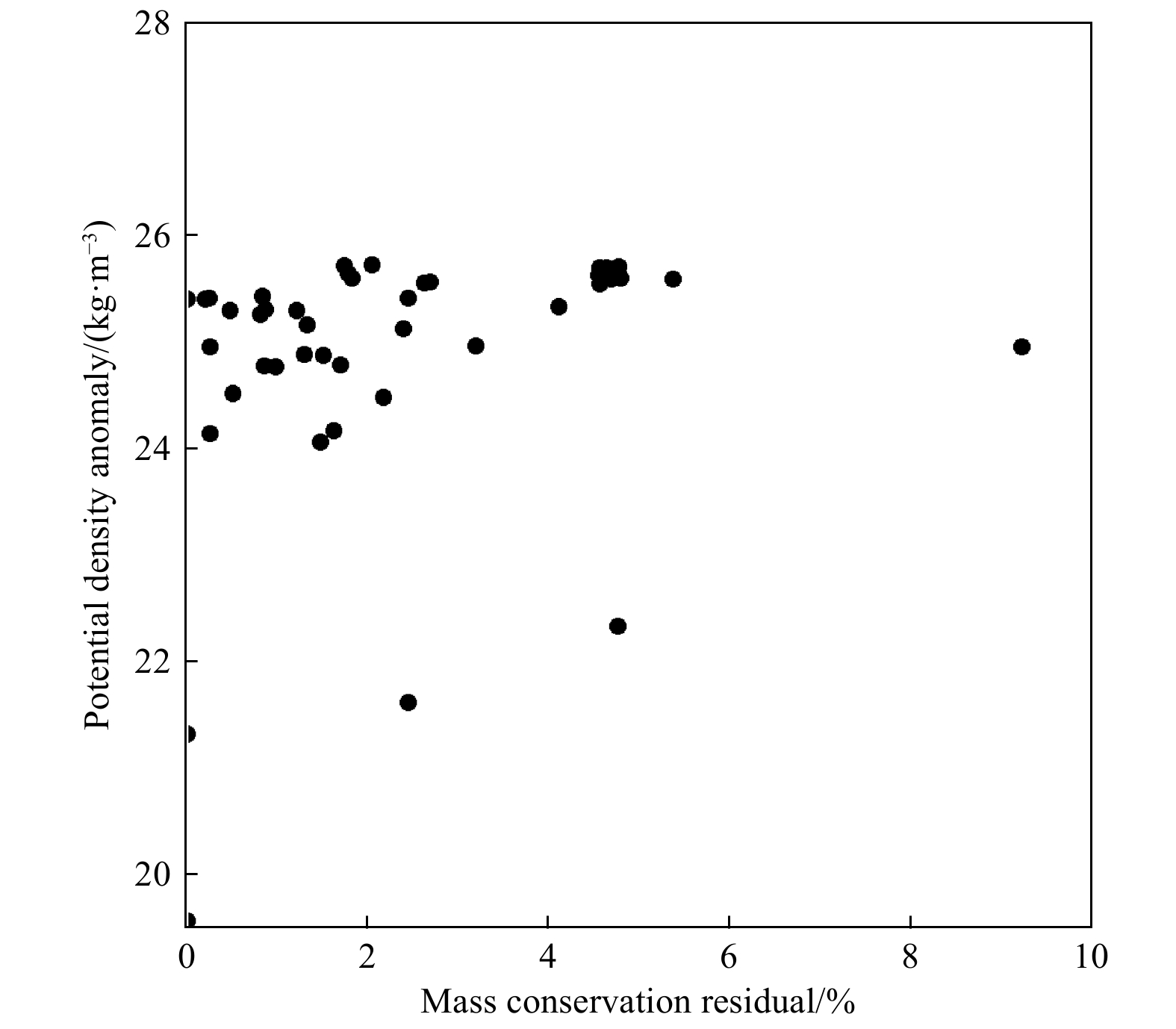
Mass conservation residuals were commonly used to evaluate the uncertainty of the OMP analysis. Traditionally, a mass conservation residual (i.e., R) of less than 7% is the standard used to measure the uncertainty of results in OMP practice (Gasparin et al., 2014; Zhou et al., 2018). As shown in Fig. 6, only one datum of R is about 9%, that means more than 97% of the conservation residuals were lower than 6% in this study. Thus, the results of the OMP analysis were reliable (Zhou et al., 2018).
It should be noted that the submarine groundwater discharge (SGD) is also an important water mass contribution to this area (Gu et al., 2012), which was not envolved as a separate end member of this study, because the water in Station D1, which was chosen as the end member of CEW, is actually a mixing water of CDW, SGD and the coastal sea water. The contributions of SGD and other water masses may be envolved in the future research to give a more accurate description of water mixing in this area. Although this study may only represent a snapshot of the water mixing in the northern part of ECS during spring, the activity ratio of 234U/238U has been successfully used as a parameter in the OMP method in the calculation of the water masses mixing in the northern ECS. This method is suitable to the marginal sea area, especially the estuarine region where the end members of water masses usually have different 234U/238U activity ratios, which is a parameter can not be altered by water column biogeochemical processes occurring in the near shore area.
In this study, 234U/238U activity ratios combined with temperature and salinity suggested that the water mass in the northern ECS is a mixture of CEW, KW and YSCC. The mixing ratios of these three water sources were calculated by the OMP method. The mass conservation residuals in the study area were lower than 6%, indicating that the running results of the OMP analysis were reliable. In spring, the dominant source water in the northern ECS was the YSCC. The CEW can only affect shallow offshore waters less than 30 m. Only the east edge of northern ECS was affected by the KW. This result suggested that the 234U/238U activity ratio as a conservative tracer is suitable to characterize and quantify the various water masses in the ECS, as well as other marginal seas influenced by different water masses with their characteristic 234U/238U activity ratios.
We are grateful to Dr. Teng Cong for the help in using MATLAB. We also thank the laboratory staff for their help during sampling and analysis. We thank the Key Laboratory of Marine Chemistry Theory and Technology of Ministry of Education for the assistance (No. 227). This is MCTL contribution No. 142.
| [1] |
Adloff J P, Roessler K. 1991. Recoil and transmutation effects in the migration behaviour of actinides. Radiochimica Acta, 52–53: 269–274
|
| [2] |
Andersen M B, Erel Y, Bourdon B. 2009. Experimental evidence for 234U-238U fractionation during granite weathering with implications for 234U/238U in natural waters. Geochimica et Cosmochimica Acta, 73(14): 4124–4141. doi: 10.1016/j.gca.2009.04.020
|
| [3] |
Budillon G, Pacciaroni M, Cozzi S, et al. 2003. An optimum multiparameter mixing analysis of the shelf waters in the Ross Sea. Antarctic Science, 15(1): 105–118. doi: 10.1017/S095410200300110X
|
| [4] |
Carroll J, Moore W S. 1993. Uranium removal during low discharge in the Ganges-Brahmaputra mixing zone. Geochimica et Cosmochimica Acta, 57(21–22): 4987–4995
|
| [5] |
Chabaux F, Riotte J, Dequincey O. 2003. U-Th-Ra fractionation during weathering and river transport. Reviews in Mineralogy and Geochemistry, 52(1): 533–576. doi: 10.2113/0520533
|
| [6] |
Chen C T A. 2009. Chemical and physical fronts in the Bohai, Yellow and East China Seas. Journal of Marine Systems, 78(3): 394–410. doi: 10.1016/j.jmarsys.2008.11.016
|
| [7] |
Chen J H, Edwards R L, Wasserburg G J. 1986. 238U, 234U and 232Th in seawater. Earth and Planetary Science Letters, 80(3–4): 241–251
|
| [8] |
Chen C T A, Ruo R, Paid S C, et al. 1995. Exchange of water masses between the East China Sea and the Kuroshio off northeastern Taiwan. Continental Shelf Research, 15(1): 19–39. doi: 10.1016/0278-4343(93)E0001-O
|
| [9] |
Cheng Hai, Edwards R L, Hoff J, et al. 2000. The half-lives of uranium-234 and thorium-230. Chemical Geology, 169(1–2): 17–33
|
| [10] |
Dinauer A, Mucci A. 2018. Distinguishing between physical and biological controls on the spatial variability of pCO2: a novel approach using OMP water mass analysis (St. Lawrence, Canada). Marine Chemistry, 204: 107–120. doi: 10.1016/j.marchem.2018.03.007
|
| [11] |
Dunk R M, Mills R A, Jenkins W J. 2002. A reevaluation of the oceanic uranium budget for the Holocene. Chemical Geology, 190(1–4): 45–67
|
| [12] |
Fleischer R L. 1980. Isotopic disequilibrium of uranium: alpha-recoil damage and preferential solution effects. Science, 207(4434): 979–981. doi: 10.1126/science.207.4434.979
|
| [13] |
Gasparin F, Maes C, Sudre J, et al. 2014. Water mass analysis of the coral sea through an optimum multiparameter method. Journal of Geophysical Research: Oceans, 119(10): 7229–7244. doi: 10.1002/2014JC010246
|
| [14] |
Gu Hequan, Moore W S, Zhang Lei, et al. 2012. Using radium isotopes to estimate the residence time and the contribution of submarine groundwater discharge (SGD) in the Changjiang effluent plume, East China Sea. Continental Shelf Research, 35: 95–107. doi: 10.1016/j.csr.2012.01.002
|
| [15] |
Guo Laodong, Warnken K W, Santschi P H. 2007. Retention behavior of dissolved uranium during ultrafiltration: implications for colloidal U in surface waters. Marine Chemistry, 107(2): 156–166. doi: 10.1016/j.marchem.2007.06.017
|
| [16] |
Han I S, Kamio K, Matsuno T, et al. 2001. High frequency current fluctuations and cross-shelf flows around the pycnocline near the shelf break in the East China Sea. Journal of Oceanography, 57(2): 235–249. doi: 10.1023/A:1011199325842
|
| [17] |
Helland-Hansen B J. 1916. Nogen hydrografiske metoder. Forh Skaudinavioke Naturf Mӧte, 16: 357–359
|
| [18] |
Ho Chongben, Wang Yuanxiang, Lei Zongyou, et al. 1959. A prelimenary study of the formation of Yellow Sea Cold Mass and its properties. Oceanologia et Limnologia Sinica (in Chinese), 2(1): 11–15
|
| [19] |
Iseki K, Okamura K, Kiyomoto Y. 2003. Seasonality and composition of downward particulate fluxes at the continental shelf and Okinawa Trough in the East China Sea. Deep Sea Research Part II: Topical Studies in Oceanography, 50(2): 457–473. doi: 10.1016/S0967-0645(02)00468-X
|
| [20] |
Jacobsen J P. 1927. Eine graphsche methode zur bestimmung des vermischungs-koeffzienten in meere. Gerlands Beitrage Geophsik, 16: 404–412
|
| [21] |
Jiang Xueyan, Yu Zhigang, Ku T L, et al. 2007. Behavior of uranium in the Yellow River plume (Yellow river estuary). Estuaries and Coasts, 30(6): 919–926. doi: 10.1007/BF02841385
|
| [22] |
Kigoshi K. 1971. Alpha-Recoil thorium-234: dissolution into water and the uranium-234/uranium-238 disequilibrium in nature. Science, 173(3991): 47–48. doi: 10.1126/science.173.3991.47
|
| [23] |
Klein B, Tomczak M. 1994. Identification of diapycnal mixing through optimum multiparameter analysis: 2. Evidence for unidirectional diapycnal mixing in the front between North and South Atlantic Central Water. Journal of Geophysical Research: Oceans, 99(C12): 25275–25280. doi: 10.1029/94JC01948
|
| [24] |
Ku T L, Knauss K G, Mathieu G G. 1977. Uranuim in open ocean: concentration and isotopic composition. Deep Sea Research, 24(11): 1005–1017
|
| [25] |
Li Wenjian, Wang Zhenyan, Huang Haijun. 2019. Relationship between the southern Yellow Sea Cold Water Mass and the distribution and composition of suspended particulate matter in summer and autumn seasons. Journal of Sea Research, 154: 101812. doi: 10.1016/j.seares.2019.101812
|
| [26] |
Lian Ergang, Yang Shouye, Wu Hui, et al. 2016. Kuroshio subsurface water feeds the wintertime Taiwan warm current on the inner East China Sea shelf. Journal of Geophysical Research: Oceans, 121(7): 4790–4803. doi: 10.1002/2016JC011869
|
| [27] |
Lie H J, Cho C H. 2016. Seasonal circulation patterns of the Yellow and East China Seas derived from satellite-tracked drifter trajectories and hydrographic observations. Progress in Oceanography, 146: 121–141. doi: 10.1016/j.pocean.2016.06.004
|
| [28] |
Liu Qian, Jiang Xueyan, Sui Juanjuan, et al. 2018. Role of suspended particulate matter in regulating the behavior of dissolved uranium in the Yellow River estuary. Estuaries and Coasts, 41(6): 1667–1678. doi: 10.1007/s12237-018-0392-9
|
| [29] |
Liu Wei, Song Jinming, Yuan Huamao, et al. 2017. Dissolved barium as a tracer of Kuroshio incursion in the Kuroshio region east of Taiwan Island and the adjacent East China Sea. Science China: Earth Sciences, 60(7): 1356–1367. doi: 10.1007/s11430-016-9039-7
|
| [30] |
Liu Jingpu, Xu Kehui, Li Anchun, et al. 2007. Flux and fate of Yangtze River sediment delivered to the East China Sea. Geomorphology, 85(3–4): 208–224
|
| [31] |
Maamaatuaiahutapu K, Garçon V C, Provost C, et al. 1992. Brazil-Malvinas confluence: water mass composition. Journal of Geophysical Research: Oceans, 97(C6): 9493–9505. doi: 10.1029/92JC00484
|
| [32] |
Maamaatuaiahutapu K, Garçon V C, Provost C, et al. 1994. Spring and winter water mass composition in the Brazil–Malvinas Confluence. Journal of Marine Research, 52(3): 397–426. doi: 10.1357/0022240943077064
|
| [33] |
Mackas D L, Denman K L, Bennett A F. 1987. Least squares multiple tracer analysis of water mass composition. Journal of Geophysical Research: Oceans, 92(C3): 2907–2918. doi: 10.1029/JC092iC03p02907
|
| [34] |
McKee B A, DeMaster D J, Nittrouer C A. 1987. Uranium geochemistry on the Amazon shelf: evidence for uranium release from bottom sediments. Geochimica et Cosmochimica Acta, 51(10): 2779–2786. doi: 10.1016/0016-7037(87)90157-8
|
| [35] |
Moore W S, Shaw T J. 2008. Fluxes and behavior of radium isotopes, barium, and uranium in seven Southeastern US rivers and estuaries. Marine Chemistry, 108(3–4): 236–254
|
| [36] |
Pardo P C, Pérez F F, Velo A, et al. 2012. Water masses distribution in the Southern Ocean: improvement of an extended OMP (eOMP) analysis. Progress in Oceanography, 103: 92–105. doi: 10.1016/j.pocean.2012.06.002
|
| [37] |
Poole R, Tomczak M. 1999. Optimum Multiparameter analysis of the water mass structure in the Atlantic Ocean thermocline. Deep Sea Research Part I: Oceanographic Research Papers, 46(11): 1895–1921. doi: 10.1016/S0967-0637(99)00025-4
|
| [38] |
Porcelli D, Andersson P S, Wasserburg G J, et al. 1997. The importance of colloids and mires for the transport of uranium isotopes through the Kalix River watershed and Baltic Sea. Geochimica et Cosmochimica Acta, 61(19): 4095–4113. doi: 10.1016/S0016-7037(97)00235-4
|
| [39] |
Porcelli D, Andersson P S, Baskaran M, et al. 2001. Transport of U-and Th-series nuclides in a Baltic shield watershed and the Baltic Sea. Geochimica et Cosmochimica Acta, 65(15): 2439–2459. doi: 10.1016/S0016-7037(01)00610-X
|
| [40] |
Qi Jifeng, Yin Baoshu, Zhang Qilong, et al. 2014. Analysis of seasonal variation of water masses in East China Sea. Chinese Journal of Oceanology and Limnology, 32(4): 958–971. doi: 10.1007/s00343-014-3269-1
|
| [41] |
Robinson L F, Belshaw N S, Henderson G M. 2004. U and Th concentrations and isotope ratios in modern carbonates and waters from the Bahamas. Geochimica et Cosmochimica Acta, 68(8): 1777–1789. doi: 10.1016/j.gca.2003.10.005
|
| [42] |
Shen Chuanchou, Edwards R L, Cheng Hai, et al. 2002. Uranium and thorium isotopic and concentration measurements by magnetic sector inductively coupled plasma mass spectrometry. Chemical Geology, 185(3–4): 165–178
|
| [43] |
Su Yusong, Li Fengqi, Ma Helai, et al. 1989. Formation and seasonal variation of bottom cold water mass in northern area of the East China Sea. Journal of Ocean University of Qingdao (in Chinese), (S1): 1–14
|
| [44] |
Sui Juanjuan, Yu Zhigang, Xu Bochao, et al. 2014. Concentrations and fluxes of dissolved uranium in the Yellow River estuary: seasonal variation and anthropogenic (Water-Sediment Regulation Scheme) impact. Journal of Environmental Radioactivity, 128: 38–46. doi: 10.1016/j.jenvrad.2013.11.003
|
| [45] |
Swarzenski P W, McKee B A. 1998. Seasonal uranium distributions in the coastal waters off the Amazon and Mississippi rivers. Estuaries, 21(3): 379–390. doi: 10.2307/1352837
|
| [46] |
Swarzenski P W, McKee B A, Booth J G. 1995. Uranium geochemistry on the Amazon shelf: chemical phase partitioning and cycling across a salinity gradient. Geochimica et Cosmochimica Acta, 59(1): 7–18. doi: 10.1016/0016-7037(94)00371-R
|
| [47] |
Tan Ehui, Wang Guizhi, Moore W S, et al. 2018. Shelf-scale submarine groundwater discharge in the Northern South China Sea and East China Sea and its geochemical impacts. Journal of Geophysical Research: Oceans, 123(4): 2997–3013. doi: 10.1029/2017JC013405
|
| [48] |
Thompson R O R Y, Edwards R J. 1981. Mixing and water-mass formation in the Australian Subantarctic. Journal of Physical Oceanography, 11(10): 1399–1406. doi: 10.1175/1520-0485(1981)011<1399:MAWMFI>2.0.CO;2
|
| [49] |
Tomczak Jr M. 1981. A multi-parameter extension of temperature/salinity diagram techniques for the analysis of non-isopycnal mixing. Progress in Oceanography, 10(3): 147–171. doi: 10.1016/0079-6611(81)90010-0
|
| [50] |
Tomczak M. 1999. Some historical, theoretical and applied aspects of quantitative water mass analysis. Journal of Marine Research, 57(2): 275–303. doi: 10.1357/002224099321618227
|
| [51] |
Tomczak M, Large D G B. 1989. Optimum multiparameter analysis of mixing in the thermocline of the eastern Indian Ocean. Journal of Geophysical Research: Oceans, 94(C11): 16141–16149. doi: 10.1029/JC094iC11p16141
|
| [52] |
Tomczak M, Liefrink S. 2005. Interannual variations of water mass volumes in the Southern Ocean. Journal of Atmospheric & Ocean Science, 10(1): 31–42
|
| [53] |
Wang Xilong, Baskaran M, Su Kaijun, et al. 2018. The important role of submarine groundwater discharge (SGD) to derive nutrient fluxes into river dominated ocean margins—the East China Sea. Marine Chemistry, 204: 121–132. doi: 10.1016/j.marchem.2018.05.010
|
| [54] |
Wang Jinlong, Du Jinzhou, Baskaran M, et al. 2016. Mobile mud dynamics in the East China Sea elucidated using 210Pb, 137Cs, 7Be, and 234Th as tracers. Journal of Geophysical Research: Oceans, 121(1): 224–239. doi: 10.1002/2015JC011300
|
| [55] |
Wang Jinlong, Fan Yukun, Liu Dantong, et al. 2019. Spatial and vertical distribution of 129I and 127I in the East China Sea: Inventory, source and transportation. Science of the Total Environment, 652: 177–188. doi: 10.1016/j.scitotenv.2018.10.248
|
| [56] |
Wang Lisheng, Ma Zhibang, Sun Zhilei, et al. 2017. U concentration and 234U/238U of seawater from the Okinawa Trough and Indian Ocean using MC-ICPMS with SEM protocols. Marine Chemistry, 196: 71–80. doi: 10.1016/j.marchem.2017.08.001
|
| [57] |
Wei Qinsheng, Wang Huiwu, Ge Renfeng, et al. 2013. Chemical hydrography and seasonal succession in the border between Yellow Sea and East China Sea. Oceanologia et Limnologia Sinica (in Chinese), 44(5): 1170–1181
|
| [58] |
Yanao S, Matsuno T. 2013. Characteristics of outer shelf water in the East China Sea. Journal of Oceanography, 69(2): 245–258. doi: 10.1007/s10872-012-0169-x
|
| [59] |
Yang Shilun, Zhang Jianmin, Zhu J, et al. 2005. Impact of dams on Yangtze River sediment supply to the sea and delta intertidal wetland response. Journal of Geophysical Research: Earth Surface, 110(F3): F03006
|
| [60] |
Zhang Jing, Liu Qian, Bai Lili, et al. 2018. Water mass analysis and contribution estimation using heavy rare earth elements: significance of Kuroshio intermediate water to Central East China Sea shelf water. Marine Chemistry, 204: 172–180. doi: 10.1016/j.marchem.2018.07.011
|
| [61] |
Zhang Liren, Liu Zhe, Zhang Jianmin, et al. 2007. Reevaluation of mixing among multiple water masses in the shelf: an example from the East China Sea. Continental Shelf Research, 27(15): 1969–1979. doi: 10.1016/j.csr.2007.04.002
|
| [62] |
Zhao Lijun, Liu Dantong, Wang Jinlong, et al. 2018. Spatial and vertical distribution of radiocesium in seawater of the East China Sea. Marine Pollution Bulletin, 128: 361–368. doi: 10.1016/j.marpolbul.2018.01.047
|
| [63] |
Zhou Jing, Du Jinzhou, Bi Qianqian, et al. 2016. The importance of the suspended sediment for the uranium non-conservative behavior in the Changjiang Estuary. Haiyang Xuebao (in Chinese), 38(12): 46–54
|
| [64] |
Zhou Jing, Du Jinzhou, Moore W S, et al. 2015. Concentrations and fluxes of uranium in two major Chinese rivers: the Changjiang River and the Huanghe River. Estuarine, Coastal and Shelf Science, 152: 56–64. doi: 10.1016/j.ecss.2014.11.004
|
| [65] |
Zhou Peng, Song Xiuxian, Yuan Yongquan, et al. 2018. Water mass analysis of the East China Sea and interannual variation of Kuroshio subsurface water intrusion through an optimum multiparameter method. Journal of Geophysical Research: Oceans, 123(5): 3723–3738. doi: 10.1029/2018JC013882
|


Figures(6) / Tables(1)

Supported by:
Beijing Renhe Information Technology Co. Ltd


| Water masses | ω | |||
| CEW | KW | YSCC | ||
| Salinity | 25.81 | 34.81 | 32.15 | 3.5 |
| Temperature/°C | 11.37 | 24.47 | 9.64 | 1.9 |
| 234U/238U activity ratio | 1.170 7 | 1.148 1 | 1.158 4 | 0.005 0 |
| Note: ω is the standard deviation of each property. CEW: estuarine water of Changjiang River, KW: Kuroshio water, YSCC: Yellow Sea Coastal Current. | ||||
DownLoad:
CSV
 DownLoad:


 DownLoad:


