Guanbao Li, Jingqiang Wang, Xiangmei Meng, Baohua Liu, Guangming Kan, Guozhong Han, Qingfeng Hua, Yanliang Pei, Lei Sun. Relationships between the sound speed ratio and physical properties of surface sediments in the South Yellow Sea[J]. Acta Oceanologica Sinica, 2021, 40(4): 65-73. doi: 10.1007/s13131-021-1764-8
Citation:
Guanbao Li, Jingqiang Wang, Xiangmei Meng, Baohua Liu, Guangming Kan, Guozhong Han, Qingfeng Hua, Yanliang Pei, Lei Sun. Relationships between the sound speed ratio and physical properties of surface sediments in the South Yellow Sea[J]. Acta Oceanologica Sinica, 2021, 40(4): 65-73. doi: 10.1007/s13131-021-1764-8
Guanbao Li, Jingqiang Wang, Xiangmei Meng, Baohua Liu, Guangming Kan, Guozhong Han, Qingfeng Hua, Yanliang Pei, Lei Sun. Relationships between the sound speed ratio and physical properties of surface sediments in the South Yellow Sea[J]. Acta Oceanologica Sinica, 2021, 40(4): 65-73. doi: 10.1007/s13131-021-1764-8
Citation:
Guanbao Li, Jingqiang Wang, Xiangmei Meng, Baohua Liu, Guangming Kan, Guozhong Han, Qingfeng Hua, Yanliang Pei, Lei Sun. Relationships between the sound speed ratio and physical properties of surface sediments in the South Yellow Sea[J]. Acta Oceanologica Sinica, 2021, 40(4): 65-73. doi: 10.1007/s13131-021-1764-8
Key Laboratory of Marine Geology and Metallogeny, First Institute of Oceanography, Ministry of Natural Resources, Qingdao 266061, China
2.
Laboratory for Marine Geology, Pilot National Laboratory for Marine Science and Technology (Qingdao), Qingdao 266237, China
3.
National Deep Sea Center, Ministry of Natural Resources, Qingdao 266237, China
Funds:
The National Natural Science Foundation of China under contract Nos 42076082, 41706062 and 41676055; the Director Fund of Pilot National Laboratory for Marine Science and Technology (Qingdao) under contract No. QNLM201713; the Public Science and Technology Research Funds Projects of Ocean under contract No. 201405032; the Taishan Scholar Project Funding under contract No. tspd20161007.
Building empirical equations is an effective way to link the acoustic and physical properties of sediments. These equations play an important role in the prediction of sediments sound speeds required in underwater acoustics. Although many empirical equations coupling acoustic and physical properties have been developed over the past few decades, further confirmation of their applicability by obtaining large amounts of data, especially for equations based on in situ acoustic measurement techniques, is required. A sediment acoustic survey in the South Yellow Sea from 2009 to 2010 revealed statistical relationships between the in situ sound speed and sediment physical properties. To improve the comparability of these relationships with existing empirical equations, the present study calculated the ratio of the in situ sediment sound speed to the bottom seawater sound speed, and established the relationships between the sound speed ratio and the mean grain size, density and porosity of the sediment. The sound speed of seawater at in situ measurement stations was calculated using a perennially averaged seawater sound speed map by an interpolation method. Moreover, empirical relations between the index of impedance and the sound speed and the physical properties were established. The results confirmed that the existing empirical equations between the in situ sound speed ratio and the density and porosity have general suitability for application. This study also considered that a multiple-parameter equation coupling the sound speed ratio to both the porosity and the mean grain size may be more useful for predicting the sound speed than an equation coupling the sound speed ratio to the mean grain size.
The seabed is one of the important boundaries for acoustic propagation in the ocean, especially in shallow seas. As the basic parameter for underwater acoustic study, the sediment sound speed is conventionally obtained by direct measurement methods, including laboratory and in situ measurements and acoustic inversion (e.g., Hamilton et al., 1956; Hamilton, 1963; Zhou et al., 2009, Yang and Tang, 2017; Wang et al., 2018). Additionally, many studies have established the empirical or theoretical models for sound speed prediction (e.g., Biot, 1956a, b; Hamilton, 1971; Stoll, 1977; Hamilton and Bachman, 1982; Buckingham, 2000, 2007; Williams, 2001; Chotiros and Isakson, 2004, 2014; Kimura, 2011). The sound speed of sediment are related to the temperature and pressure; therefore, the sound speed ratio, which is defined as the ratio of the sound speed in sediment to that in seawater under the same conditions (temperature, pressure and salinity), was suggested to eliminate the effects of temperature and pressure (Hamilton, 1971). The sound speed ratio is widely used in theoretical and empirical prediction models, especially the latter (Hamilton and Bachman, 1982; Jackson and Richardson, 2007).
The most widely used empirical equations were established by Hamilton and Bachman (1982) to predict the sound speed based on the density, porosity and mean grain size of sediment and later modified by Bachman (1989) for the sound speed ratio against the same three parameters (this set of equations is referred to hereafter the H&B model). Then, in the 1990s, with the successive development of in situ measurement systems such as the in situ sediment acoustic measurement system (ISSAMS) and acoustic lance (Richardson and Briggs, 1996; Fu et al., 1996), the “undisturbed” sediment acoustic properties were able to be obtained under real seafloor conditions. Subsequently, empirical regressions were proposed for in situ sound speed ratio prediction based on the sediment density, porosity and grain size (Richardson, 1997; Jackson and Richardson, 2007) (these equations are hereafter referred as the J&R model). However, the J&R model yields a lower sound speed ratio value than that predicted by the H&B model. Jackson and Richardson (2007) argued that the differences between the two models may be due to the measurement techniques of acoustic property and physical property, sample perturbations, or even actual differences in the sediment. Uncertainty about differences among various models makes it difficult to choose the appropriate model for predictions. Comparatively, the J&R model seems to be more suitable for prediction in that the sound speed ratio data are derived from the in-situ measurement technique and are believed to be less affected by the variation in measurement conditions than the laboratory method. Nevertheless, the J&R model was based only on 88 sites (Jackson and Richardson, 2007), and more data are necessary to confirm it, especially data measured using in situ techniques.
The South Yellow Sea (SYS) is an epicontinental sea in the western Pacific margin. Abundant terrestrial materials, delivered by the surrounding large rivers, are deposited and then reworked under the unique ocean circulation system in the SYS (Shi, 2012). In 2009 and 2010, two cruises of sediment acoustic survey (named YSSA09 and YSSA10) were conducted in the central and western parts of the SYS (Fig. 1a) to characterize the distribution of sediment acoustic and physical properties. A hydraulically driven self-contained in situ sediment acoustic measurement system (named HISAMS by Liu et al. (2013)) was used to acquire the sound speed of the sediment at 104 stations. The center measurement frequency of this system was 30 kHz. Sediment samples were collected for physical property measurements in the laboratory. The data made it possible to build empirical equations to compare with the previous models. Liu et al. (2013) published the in situ acoustic and physical property data and established regression equations of the in situ sound speed against the mean grain size, density and porosity. However, during the two survey, the bottom seawater sound speed measurements were performed at only a few stations, which was not sufficient for calculating the in situ sound speed ratio at each station. Therefore, the sound speed ratio prediction model was not provided, although the bottom seawater temperatures in the study region are variable (Fig. 1b, based on Editorial Board for Marine Atlas (EBMA), 1993). To accommodate the lack of data for the sound speed ratio calculations mentioned above, this study accessed the historical data of seawater sound speed in the SYS (Editorial Board for Marine Atlas, 1993) and used the sound speed of the bottom seawater to calculate the sound speed ratio at each in situ station. Then, the relationships between the sound speed ratio and physical properties were established and compared with the previous models.
Figure
1.
The location of the study area (a, red shaded area), contour map of the bottom seawater temperature (°C) in the study area in June (b, from Editorial Board for Marine Atlas, 1993), and contour map of the bottom seawater sound speed (m/s) in the study area in June (c, from Editorial Board for Marine Atlas, 1993). In a, the black shaded area shows the study area of Kim et al. (2011) and Bae et al. (2014), whose data were used for comparison. BS: Bohai Sea, NYS: North Yellow Sea, SYS: South Yellow Sea, ECS: East China Sea, KWC: Kuroshio Warm Current, YSWC: Yellow Sea Warm Current, YSCC: Yellow Sea Coastal Current, and KCC: Korea Coastal Current.
The data used in this study are from the two cruises of YSSA09 and YSSA10, including the in situ sediment sound speed and the physical properties measured in laboratory, such as the mean grain size, density, porosity, and sand, silt, and clay content (Meng et al., 2012). The in situ sound speed were measured by the self-contained HISAMS, in which the acoustic transducers are inserted into the sediment by a hydraulic system and then transmit and receive sound wave signals in the sediment. The arrival time of the received sound wave signals and the distances between probes are used to determine the sound speed of the sediment. For a detailed description of the self-contained HISAMS, please refer to Kan et al. (2011). Liu et al. (2013) also described the methodology of in situ sound speed measurement and data processing, and a measurement accuracy of approximately 0.5% was acquired by calibration in the seawater using conductivity temperature depth sensors (CTD). Notably, the HISAMS utilizes a similar working style as the ISSAMS, which penetrates the transmitter and receivers into same depth below the seafloor and performs measurements in the horizontal direction. Therefore, the measurement results of the HISAMS were more comparable with those of the ISSAMS than the cross-layer averaged sound speed taken from measurements in the vertical direction (such as acoustic lance).
The sediment samples were collected by a gravity corer or a box sampler. However, sample collecting are unavailable at some stations due to the hard seabed. Therefore, only the in situ stations with available sediment samples were included in Liu et al. (2013). Each sample was then measured in the laboratory by conventional methods to acquire physical properties such as density, porosity, grain size, and particle composition. Test methods for physical properties were described in detail by Liu et al. (2013) and will not be reiterated here. As the HISAMS has no sediment sampling function, sample collection is performed before or after the in situ measurement. Although the research vessel was anchored each time before station operation, the vessel tended to drift an average of 10 m between measurements. As a result, the position of the in situ measurement was not strictly consistent with the sampling position.
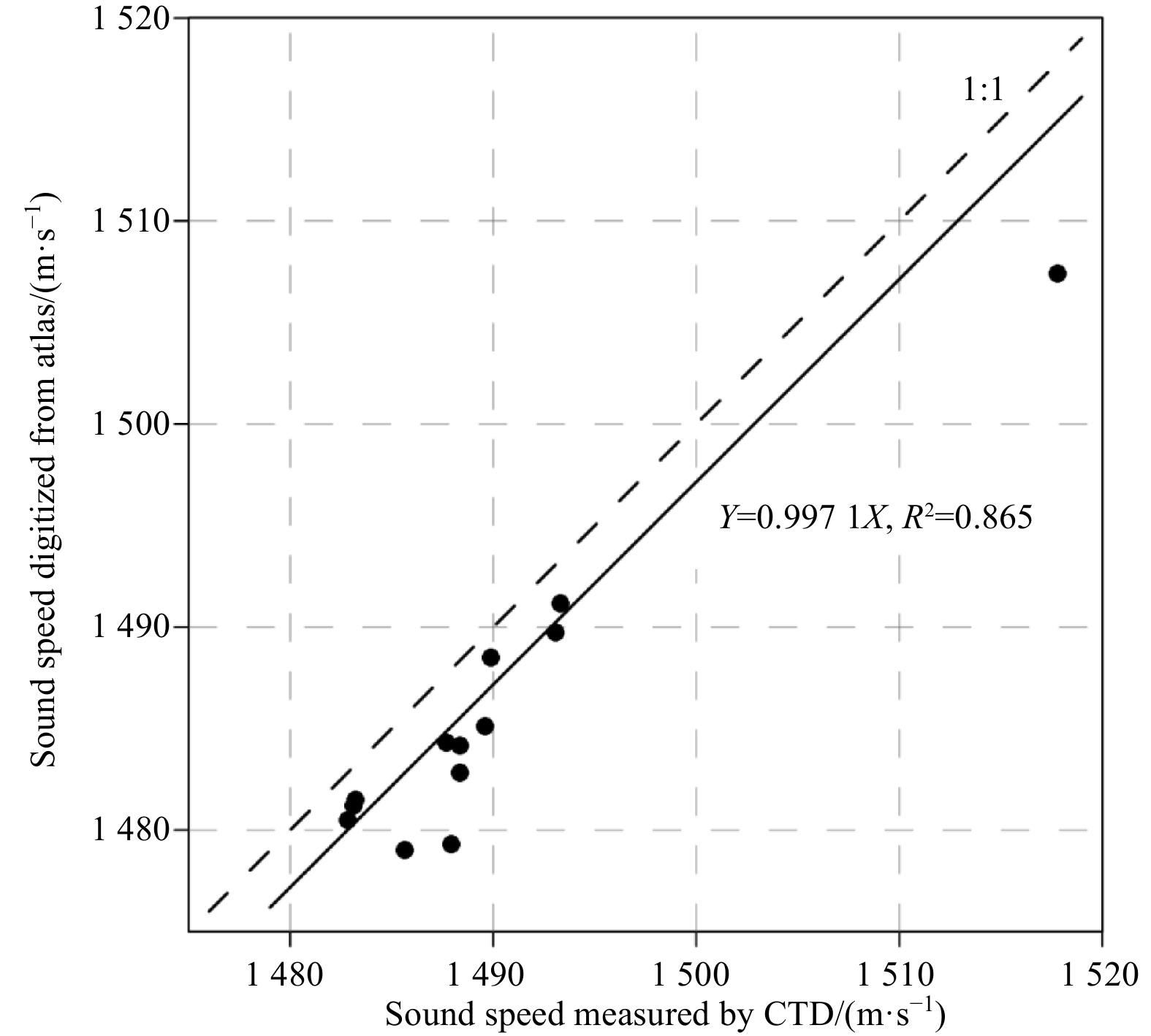
The YSSA09 and YSSA10 collected seawater sound speed profiles using CTD at a total of 13 stations that were fairly evenly distributed in the study region. For these stations, the sound speed ratios were calculated using the measured sound speed of sediments and seawater. For other stations without measured seawater sound speed, the Marine Atlas of the Bohai Sea, Huanghai Sea, East China Sea (Hydrology) (Editorial Board for Marine Atlas, 1993) was used to deduce seawater sound speed data for the sound speed ratio calculation. Both YSSA09 and YSSA10 were carried out in June, so the contour map of the bottom seawater sound speed in June (Fig. 1c) in the atlas was selected and digitized according to its projection method (Mercator Projection). Then, the sound speed value on the corresponding position of the in situ measurement station was calculated by an interpolation method. Compared to the measured sound speed at the bottom of the CTD profile, the digitally interpolated seawater speed at the same station shows a general consistency (Fig. 2), with a slight difference that averages less than 0.3%, which indicates that it is appropriate to use the hydrology atlas to obtain the sound speed of the bottom seawater.
Figure
2.
Comparison of the bottom seawater sound speed interpolated from the hydrology atlas to that measured by CTD during the cruises. The 1:1 dashed line represents that the sound speed is equal, and the solid line is the fitting curve.
The relationships between the sound speed ratio and the mean grain size, density and porosity were built by quadratic equation fitting, and the correlation coefficient was obtained to evaluate the goodness of fit. Additionally, the index of acoustic impedance (IOI) was calculated by multiplying the sound speed ratio and density, and then the empirical equations between the main physical property parameter and the IOI were established by the polynomial regression method.
3.
Results
3.1
Sound speed ratio and its empirical regressions versus physical properties
The calculated sound speed ratio ranges from 0.967 to 1.074 and its upper limit is lower than that of the in situ sound speed ratio in Jackson and Richardson (2007), which is more than 1.15. There are coarse sand deposits in the southwestern part of the study area according to the sediment type atlas (Shi, 2012), but sediment samples were obtained in only a few stations due to the hard seabed. As a result, the types of sediment samples are dominated mainly by silt and clay, as shown in the Shepard ternary diagram (Fig. 3), and only a few stations with sandy sediment samples are included. These factors might explain why a relatively lower sound speed ratio was acquired in this study.
Figure
3.
Shepard ternary diagram of sediment types in the study area. The black points represent the data used in this paper and the red points represent the collected data from Bae et al. (2014).
The regressions of the sound speed ratio V pR against the mean grain size Mz, density ρ, and porosity η are listed in Table 1 and the corresponding curves are plotted in Figs 4a, b and c, respectively. The sound speed ratio increases with increasing density and mean grain size (decreasing $\phi$ values) and decreases with increasing porosity, showing the same tendency as the relationship between the sound speed and these physical properties in Liu et al. (2013). The correlation coefficient of the equation between the sound speed ratio and the mean grain size is significantly lower than that of the other two equations. The data points are more scattered for the coarser particle deposits (low $\phi $ values, high density, low porosity) than for the fine particle deposits, meaning that the uncertainty of the correlation increased with increasing sound speed ratio. This is understandable, considering the difficulties in sampling and storing coarse-grained sediment, which is easily disturbed and dehydrated. Another reason for the relatively high scatter of these data points may be due to the disagreement in the sampling position and in situ measurement position, as mentioned previously. Ideally, if the sediment is sampled synchronously when the in situ measurement device is deployed, the positions of both operations will be kept identical. Therefore, the columnar sampler should be installed on the newly developed in situ measurement system, which makes it possible to collect sediment samples and deploy in situ measurements of sound properties simultaneously.
Table
1.
Empirical relationships of the sediment sound speed ratio with physical properties
Figure
4.
Relationship between the sound speed ratio and the three physical properties of mean grain size (a), bulk density (b), and porosity (c). Black points represent our data, and black solid lines represent their fitted curves, corresponding to equations listed in Table 1. Also plotted are the curves of the H&B model (blue lines), the J&R model (pink lines) as listed in Appendix, and data from Kim et al. (2011) (green diamonds) and Bae et al. (2014) (red triangles).
3.2
Index of acoustic impedance and its empirical regressions against physical properties
Using acoustic instruments such as sub-bottom profilers and multibeam echosounders, acoustic classification of the sediment can be accomplished based on the echo signals obtained and the relationship between the sediment acoustic impedance and physical properties. Richardson and Briggs (1993, 2004) proposed the concept of the index of acoustic impedance (IOI) and established its relationship with the major physical properties of sediment. The IOI was defined as the product of sound speed ratio and the bulk density, which is different from the acoustic impedance in that it is temperature independent. Considering the specific aspects of the sedimentary environment in the SYS, we also calculated the IOI using the calculated in situ sound speed ratio and the density and established the relationships of the IOI with the major sediment physical properties by the polynomial regression method, as in the quadratic equations shown in Table 2 and the curves in Fig. 6.
Table
2.
Empirical relationships between the index of impedance (IOI) and geoacoustical and physical properties
4.1
Comparison to the previous sound speed ratio empirical regressions
The equations of the H&B model and J&R model are plotted in Fig. 4. All the equations of the H&B model show an overestimation of the sound speed ratio for three physical properties in comparison to those of the J&B model and our model, while the latter two models show relatively consistent values for the density and porosity (Figs 4b and c). Moreover, our model yields a sound speed ratio that is lower than those in the H&B and J&R model for a given mean grain size (Fig. 4a).
Considering the good agreement between our model and the J&R model for the density and porosity and their disagreement for the mean grain size, we investigated whether the relationship between the porosity (or density) and the mean grain size is different between our model and the J&R model. Since the regression equation between the porosity and mean grain size was not reported by Jackson and Richardson (2007), we determined this equation by combining the equation coupling the sound speed ratio to the mean grain size and the equation coupling the sound speed ratio to the porosity, although we are not sure to what extent this regression matches the measured values of the J&R model. As shown in Fig. 5a, the J&R model yeilds an underestimation of porosity for the given mean grain size, compared to our data, while the H&B model agrees well with our data, especially for fine-grained sediment. Therefore, the relationship between the porosity and mean grain size is different in various studies, which may be due to the sediment grain shape and the sea environment.
Figure
5.
Relationship between the porosity and the mean grain size (a), and double-parameters relationship of sound speed ratio with both porosity and mean grain size (b). In a, black points represent our data; also plotted are the H&B model (blue lines), the J&R model (pink lines), and data from Bae et al. (2014) (red triangles).
Table 1 indicates that the correlation between the sound speed ratio and mean grain size is not very close, and the R-square value is indeed low. Therefore, we attempted to combine the porosity and the mean grain size to establish a two-parameter empirical equation for predicting the sound speed ratio, as listed in Table 1 and shown in Fig. 5b. With this two-parameter empirical equation, the R-square value is improved compared to that of the single-parameter equation using the mean grain size. These results indicate that the development of multiple-parameter equations would be useful for sound speed prediction.
To further confirm the above analysis, sediment acoustic measurement data of the adjacent area of the SYS, mainly the southeastern SYS off the Korean Peninsula (Fig. 1a), were collected, including the sound speed and density data published by Kim et al. (2011) and the sound speed, mean grain size, density, and porosity data published by Bae et al. (2014). However, only the sound speed was given in these articles, and the sound speed ratio was not mentioned. In addition, the above studies converted the sound speed to that of standard laboratory conditions (23°C, 1 atmosphere, and 35 salinity) as proposed by Hamilton (1971). Therefore, the seawater sound speed of 1 529.6 m/s in such a standard condition is used to calculate the corresponding sound speed ratio. Since both Kim et al. (2011) and Bae et al. (2014) focused on the so-called Central South Sea Mud region, the sediment types were mainly clayey silt, as exhibited in Fig. 3 (red points), with physical properties of low density, high porosity and small mean grain size. These collected data are also plotted in Fig. 4. The data of both Kim et al. (2011) and Bae et al. (2014) match well to our model and the J&R model. Therefore, the general suitability of the J&R model in this sea area is further confirmed. However, the sound speed ratio data of Bae et al. (2014) match better to our model using the mean grain size than the J&R model (shown in Fig. 4a), which indicates that the regression of the sound speed ratio to the mean grain size of the J&R model is not applicable for the SYS and its adjacent region.
The porosity and mean grain size data from Bae et al. (2014) are also plotted in Fig. 5. These data agree well with the regression equation of the H&B model and our data but depart from the equation of the J&R model. The sediment in the SYS is mainly terrigenous materials transported by the surrounding large rivers, especially the Huanghe River (Yellow River) and the Changjiang River (Yangtze River). After long-distance delivery by the river, this sediment is deposited and then reworked by the strong hydrodynamic forces of the SYS, such as circulation currents and tidal currents (Fig. 1a), and sediment of different grain sizes deposits at the delivery path, which leads to the sediment being well sorted in different areas. The sorting of the sediment in the study area is supported by geological survey data, which show that the sediment sorting coefficient is below 2 as a whole and is even less than 1.5 in the clayey sediment area (Shi, 2012). The grain size, shape and packing are key parameters affecting porosity in unconsolidated sediment (Kamann et al., 2007). Well-sorted sediment has more pore spaces unfilled by finer-grained components than poorly sorted sediment. This may explain why the regressions of the sound speed ratio and mean grain size are inconsistent between our model and the J&R model. This also supports the view that the mean grain size may not be a good indicator for the prediction of the sound speed. Nevertheless, as a geologically general and readily available sediment parameter, the mean grain size is still useful for predicting the sound speed in a specific region with a relatively sedimentary environment in areas lacking porosity or density data.
4.2
Comparison of the index of acoustic impedance empirical regressions
Comparing our IOI equations with those of Jackson and Richardson (2007), we can see that the porosity, density and sound speed ratio equations are in good agreement (Fig. 6). This was as expected, considering the consistency of this study and the J&R model regarding the equations linking the sound speed ratio with the density and porosity. Furthermore, the relationship of the IOI with the mean grain size is different, just as that of the sound speed ratio and the mean grain size. The relationship between the IOI and the sand content and clay content is drawn in Fig. 6e. By comparison, the relationship of the IOI with the sand content has a similar trend to that of the J&R model, although they are not entirely consistent.
Figure
6.
Relationship between the IOI and the geoacoustical and physical properties and comparison with equations from Jackson and Richardson (2007). a. Sound speed ratio against the IOI, b. mean grain size against the IOI, c. density against the IOI, d. porosity against the IOI, and e. sand content and clay content against the IOI (the pink line represents the regression for IOI against sand and gravel content in J&R model).
These equations of the IOI are valuable in practical applications, such as sediment classification and sound speed prediction. Conventional methods of measuring the sound speed (sampling and laboratory measurements, in situ measurements and acoustic inversion) at fixed points are inefficient; it is costly to obtain a dense data set. Moreover, sound speed prediction using the relationship of this parameter with physical properties is also challenging because of the difficulty in measuring physical parameters. Underway measurements using a sub-bottom profiler or multibeam echosounder typically operate with high efficiency. With the wide application of these convenient and efficient survey techniques and application of IOI models as above, a large amount of densely distributed acoustic properties of the seafloor sediment can be easily obtained.
5.
Summary
Based on the in situ measured sound speed and the historical seawater sound speed data in the SYS, this study calculated sound speed ratios at each in situ station of the YSSA09 and YSSA10 survey. This study also established new regression relationships between the sound speed ratio and three physical properties, including the mean grain size, density and porosity. In comparison to the previously built models, the new regressions of the sound speed ratio to the density and the sound speed ratio to the porosity show good agreement with those of Jackson and Richardson (2007), but there is some inconsistency in the equations coupling the sound speed ratio to the mean grain size between the two models. The sediment acoustic measurement data for the SYS published in other articles are consistent with these new equations and confirm the general applicability of the J&R model for sound speed ratio prediction based on density and porosity in the SYS. The mismatch of the equations coupling the sound speed ratio to the mean grain size may be related to the sediment itself due to the different sedimentary environments. Considering that the mean grain size is a geologically general and readily available sediment parameter, the equation coupling the sound speed versus the mean grain size is still useful for predicting the sound speed in a specific region where the porosity or density data are not available. In addition, regressions between the IOI and the acoustic and physical properties are also calculated, which may be applied for rapid sediment classification and sound speed prediction.
Acknowledgement
We thank the crew of R/V Dongfanghong 2 for assistance with the in situ acoustic measurements.
Bachman R T. 1989. Estimating velocity ratio in marine sediment. The Journal of the Acoustical Society of America, 86(5): 2029–2032. doi: 10.1121/1.398585
[2]
Bae S H, Kim D C, Lee G S, et al. 2014. Physical and acoustic properties of inner shelf sediments in the South Sea, Korea. Quaternary International, 344: 125–142. doi: 10.1016/j.quaint.2014.03.058
[3]
Biot M A. 1956a. Theory of propagation of elastic waves in a fluid-saturated porous solid: I. Low-frequency range. The Journal of the Acoustical Society of America, 28(2): 168–178. doi: 10.1121/1.1908239
[4]
Biot M A. 1956b. Theory of propagation of elastic waves in a fluid-saturated porous solid: II. Higher frequency range. The Journal of the Acoustical Society of America, 28(2): 179–191. doi: 10.1121/1.1908241
[5]
Buckingham M J. 2000. Wave propagation, stress relaxation, and grain-to-grain shearing in saturated, unconsolidated marine sediments. The Journal of the Acoustical Society of America, 108(6): 2796–2815. doi: 10.1121/1.1322018
[6]
Buckingham M J. 2007. On pore-fluid viscosity and the wave properties of saturated granular materials including marine sediments. The Journal of the Acoustical Society of America, 122(3): 1486–1501. doi: 10.1121/1.2759167
[7]
Chotiros N P, Isakson M J. 2004. A broadband model of sandy ocean sediments: biot-Stoll with contact squirt flow and shear drag. The Journal of the Acoustical Society of America, 116(4): 2011–2022. doi: 10.1121/1.1791715
[8]
Chotiros N P, Isakson M J. 2014. Shear wave attenuation and micro-fluidics in water-saturated sand and glass beads. The Journal of the Acoustical Society of America, 135(6): 3264–3279. doi: 10.1121/1.4874955
[9]
Editorial Board for Marine Atlas. 1993. Marine Atlas of Bohai Sea, Huanghai Sea and East China Sea (Hydrology) (in Chinese). Beijing: China Ocean Press
[10]
Fu S S, Wilkens R H, Frazer L N. 1996. Acoustic lance: new in situ seafloor velocity profiles. The Journal of the Acoustical Society of America, 99(1): 234–242. doi: 10.1121/1.414506
[11]
Hamilton E L. 1963. Sediment sound velocity measurements made in situ from Bathyscaph Trieste. Journal of Geophysical Research, 68(21): 5991–5998. doi: 10.1029/JZ068i021p05991
[12]
Hamilton E L. 1971. Prediction of in-situ acoustic and elastic properties of marine sediments. Geophysics, 36(2): 266–284. doi: 10.1190/1.1440168
[13]
Hamilton E L, Bachman R T. 1982. Sound velocity and related properties of marine sediments. The Journal of the Acoustical Society of America, 72(6): 1891–1904. doi: 10.1121/1.388539
[14]
Hamilton E L, Shumway G, Menard H W, et al. 1956. Acoustic and other physical properties of shallow-water sediments off San Diego. The Journal of the Acoustical Society of America, 28(1): 1–15. doi: 10.1121/1.1908210
[15]
Jackson D R, Richardson M D. 2007. High-Frequency Seafloor Acoustics. New York: Springer
[16]
Kamann P J, Ritzi R W, Dominic D F, et al. 2007. Porosity and permeability in sediment mixtures. Groundwater, 45(4): 429–438. doi: 10.1111/j.1745-6584.2007.00313.x
[17]
Kan Guangming, Liu Baohua, Zhao Yuexia, et al. 2011. Self-contained in situ sediment acoustic measurement system based on hydraulic driving penetration. High Technology Letters, 17(3): 311–316
[18]
Kim G Y, Kim D C, Yoo D G, et al. 2011. Physical and geoacoustic properties of surface sediments off eastern Geoje Island, South Sea of Korea. Quaternary International, 230(1–2): 21–33. doi: 10.1016/j.quaint.2009.07.028
[19]
Kimura M. 2011. Velocity dispersion and attenuation in granular marine sediments: comparison of measurements with predictions using acoustic models. The Journal of the Acoustical Society of America, 129(6): 3544–3561. doi: 10.1121/1.3585841
[20]
Liu Baohua, Han Tongcheng, Kan Guangming, et al. 2013. Correlations between the in situ acoustic properties and geotechnical parameters of sediments in the Yellow Sea, China. Journal of Asian Earth Sciences, 77: 83–90. doi: 10.1016/j.jseaes.2013.07.040
[21]
Meng Xiangmei, Liu Baohua, Kan Guangming, et al. 2012. An experimental study on acoustic properties and their influencing factors of marine sediment in the southern Huanghai Sea. Acta Oceanologia Sinica (in Chinese), 34(6): 74–83
[22]
Richardson M D. 1997. In-situ, shallow-water sediments geoacoustic properties. In: Zhang R, Zhou J, eds. Shallow-Water Acoustics. Beijing: China Ocean Press, 163–170
[23]
Richardson M D, Briggs K B. 1993. On the use of acoustic impedance values to determine sediment properties. In: Pace N G, Langhorne D N, eds. Acoustic Classification and Mapping of the Seabed. Bath: Institute of Acoustics, 15–25
[24]
Richardson M D, Briggs K B. 1996. In situ and laboratory geoacoustic measurements in soft mud and hard-packed sand sediments: implications for high-frequency acoustic propagation and scattering. Geo-Marine Letters, 16(3): 196–203. doi: 10.1007/BF01204509
[25]
Richardson M D, Briggs K B. 2004. Empirical predictions of seafloor properties based on remotely measured sediment impedance. In: Porter M B, Siderius M, eds. High Frequency Ocean Acoustic Conference. Melville: AIP Press, 12–21
[26]
Shi Xuefa. 2012. China Coastal Seas-Marine Sediment (in Chinese). Beijing: China Ocean Press, 27–46
[27]
Stoll R D. 1977. Acoustic waves in ocean sediments. Geophysics, 42(4): 715–725. doi: 10.1190/1.1440741
[28]
Wang Jingqiang, Li Guanbao, Liu Baohua, et al. 2018. Experimental study of the ballast in situ sediment acoustic measurement system in South China Sea. Marine Georesources & Geotechnology, 36(5): 515–521
[29]
Williams K L. 2001. An effective density fluid model for acoustic propagation in sediments derived from Biot theory. The Journal of the Acoustical Society of America, 110(5): 2276–2281. doi: 10.1121/1.1412449
[30]
Yang Jie, Tang Dajun. 2017. Direct measurements of sediment sound speed and attenuation in the frequency band of 2–8 kHz at the target and reverberation experiment site. IEEE Journal of Oceanic Engineering, 42(4): 1102–1109. doi: 10.1109/JOE.2017.2714722
[31]
Zhou Jixun, Zhang Xuezhen, Knobles D P. 2009. Low-frequency geoacoustic model for the effective properties of sandy seabottoms. The Journal of the Acoustical Society of America, 125(5): 2847–2866. doi: 10.1121/1.3089218
Figure 1. The location of the study area (a, red shaded area), contour map of the bottom seawater temperature (°C) in the study area in June (b, from Editorial Board for Marine Atlas, 1993), and contour map of the bottom seawater sound speed (m/s) in the study area in June (c, from Editorial Board for Marine Atlas, 1993). In a, the black shaded area shows the study area of Kim et al. (2011) and Bae et al. (2014), whose data were used for comparison. BS: Bohai Sea, NYS: North Yellow Sea, SYS: South Yellow Sea, ECS: East China Sea, KWC: Kuroshio Warm Current, YSWC: Yellow Sea Warm Current, YSCC: Yellow Sea Coastal Current, and KCC: Korea Coastal Current.
Figure 2. Comparison of the bottom seawater sound speed interpolated from the hydrology atlas to that measured by CTD during the cruises. The 1:1 dashed line represents that the sound speed is equal, and the solid line is the fitting curve.
Figure 3. Shepard ternary diagram of sediment types in the study area. The black points represent the data used in this paper and the red points represent the collected data from Bae et al. (2014).
Figure 4. Relationship between the sound speed ratio and the three physical properties of mean grain size (a), bulk density (b), and porosity (c). Black points represent our data, and black solid lines represent their fitted curves, corresponding to equations listed in Table 1. Also plotted are the curves of the H&B model (blue lines), the J&R model (pink lines) as listed in Appendix, and data from Kim et al. (2011) (green diamonds) and Bae et al. (2014) (red triangles).
Figure 5. Relationship between the porosity and the mean grain size (a), and double-parameters relationship of sound speed ratio with both porosity and mean grain size (b). In a, black points represent our data; also plotted are the H&B model (blue lines), the J&R model (pink lines), and data from Bae et al. (2014) (red triangles).
Figure 6. Relationship between the IOI and the geoacoustical and physical properties and comparison with equations from Jackson and Richardson (2007). a. Sound speed ratio against the IOI, b. mean grain size against the IOI, c. density against the IOI, d. porosity against the IOI, and e. sand content and clay content against the IOI (the pink line represents the regression for IOI against sand and gravel content in J&R model).


 DownLoad:


 DownLoad:


 DownLoad: