Ze Meng, Lei Zhou, Baosheng Li, Jianhuang Qin, Juncheng Xie. Erratum to: Acta Oceanologica Sinica (2022) 41(10): 119–130DOI: 10.1007/s13131-022-2023-3The atmospheric hinder for intraseasonal sea-air interaction over the Bay of Bengal during Indian summer monsoon in CMIP6[J]. Acta Oceanologica Sinica. doi: 10.1007/s13131-022-2131-0
Citation:
Ruibo Lei, Dawei Gui, Zhuoli Yuan, Xiaoping Pang, Ding Tao, Mengxi Zhai. Characterization of the unprecedented polynya events north of Greenland in 2017/2018 using remote sensing and reanalysis data[J]. Acta Oceanologica Sinica, 2020, 39(9): 5-17. doi: 10.1007/s13131-020-1643-8
MNR Key Laboratory for Polar Science, Polar Research Institute of China, Shanghai 200136, China
2.
Chinese Antarctic Center of Surveying and Mapping, Wuhan University, Wuhan 430072, China
Funds:
The National Key Research and Development Program of China under contract Nos 2018YFA0605903 and 2016YFC1402702; the National Natural Science Foundation of China under contract Nos 41722605 and 41976219.
Based on an ice concentration threshold of 90%, it has been identified that two polynya events occurred in the region north of Greenland during the 2017/2018 ice season. The winter event lasted from February 20 to March 3, 2018 and the summer event persisted from August 2 to September 5, 2018. The minimum ice concentration derived from Advanced Microwave Scanning Radiometer 2 (AMSR2) observations was 72% and 65% during the winter and summer events, respectively. The occurrence of both events can be related to strengthened southerly winds associated with an increased east-west zonal surface level air pressure gradient across the north Greenland due to perturbation of mid-troposphere polar vortex. The relatively warm air temperature during the 2017/2018 freezing season in comparison with previous years, together with the occurrence of the winter polynya, formed favourable pre-conditions for ice field fracturing in summer, which promoted the formation of the summer polynya. Diminished southerly winds and increased cover of new ice over the open water were the dominant factors for the disappearance of the winter polynya, whereas increased ice inflow from the north was the primary factor behind the closure of the summer polynya. Sentinel-1 Synthetic Aperture Radar (SAR) images were found better suited than AMSR2 observations for quantification of a new ice product during the polynya event because the SAR images have high potential for mapping of different sea ice regimes with finely spatial resolution. The unprecedented polynya events north of Greenland in 2017/2018 are important from the perspective of Arctic sea ice loss because they occurred in a region that could potentially be the last “Arctic sea ice refuge” in future summers.
Objective analysis, a kind of techniques for gridding observations, has developed and evolved for many decades. Historically, its main purpose is to provide initial conditions for operational prediction models and aid in the diagnostic studies in atmospheric and oceanic field. Although the use for the first purpose has all but disappeared today due to the springing-up of other more sophisticated schemes such as optimal interpolation (OI) and variational methods, objective analysis schemes are still widely used for diagnostic purposes and many studies have employed various incarnations of them to investigate a diverse range of researches.
As a branch of objective analysis, successive correction menthod (SCM) represented by Cressman (1959) and Barnes (1964, 1973) have received more attention than others and remain popular today. Cressman (1959) used a series of scans with decreasing radius of influence to retrieve a broad spectrum of wavelengths from the observations. Its major contribution is introducing the practice of building details from longer to shorter waves. Barnes (1964) argued that such a scheme suffered from the disadvantage of tending to smooth out all small variations in the field. Moreover, an unstable iteration may occur in the Cressman scheme and thus an additional dissipation scheme has to be performed (e.g., Seaman, 1983; Seaman and Hutchinson, 1985; Lu and Browning, 1998). To maximize details resolved by observations, Barnes (1964) proposed a scheme similar to the Cressman method but using a different weighting function (Gaussian-type) with the weight factor (radius of influence) fixed for all passes of scan. This algorithm was then replaced by Barnes (1973) employing only two passes (one initial pass and one correction pass) with a diminished smoothing factor for the second (correction) pass. The most attractive feature of the Barnes scheme is its well-known response characteristics. By choosing the smoothing parameters, one can ascertain which range of wavelengths will be retained in the final analysis. However, the response function of the Barnes (1964, 1973) is derived under the assumption that the observations are continuous and unbounded (infinite). Practically, it is best applicable to reasonably uniform data distributions. If data are irregularly distributed, the phase of the response function will change and signals may be distorted in the analyzed field. The more sparsely and irregularly distributed the data, the less results are in accordance with the theoretical predictions (Achtemeier, 1986; Pauley and Wu, 1990; Buzzi et al., 1991). This raises the difficulty of choosing the appropriate parameters in a particular application to achieve an optimum analysis. In fact, in the situation of sparse and irregular data distribution, no single selection of the parameters can produce the most accurate analysis for all wavelengths.
As we know, an effective objective analysis scheme should at least be able to retrieve resolvable long wavelengths in data-spare areas and preserve details in data-dense areas. If multi-wavelengths are extracted simultaneously without an effective mechanism, the analysis can be seriously contaminated by noises, arising from observational errors or irregular data distribution. A practical way to relieve this problem is analyzing first for larger scales and then for shorter scales. The more accurate the long wavelengths, the less impact the noises may have on the analyzed field. Therefore, when applied to irregularly spaced data, it is advisable for analysis scheme sequentially decrease the smoothing factors as Cressman method does in order to retain the most accurate analysis of the longer wavelengths. Based upon this idea, some variational successive corrections approaches, such as the multi-grid approach, the multi-scale diffusion filter approach, etc, have proposed by scholars as listed in Table 1. Among them, Xie et al. (2005, 2010) proposed a multi-scale 3D-VAR implemented by the multi-grid technique, using a sequence of grids with different resolutions to correct different wavelengths. The analysis is interpolated between two consecutive grid level and then enter into a new analysis cycle. Strictly speaking, the multi-grid 3D-VAR is not a traditional sense of 3D-VAR because it solves a series of 3D-VAR respectively on different grid levels. If the background filed is neglected and only the observational field is considered, the multi-grid 3D-VAR then evolves into a variational objective analysis scheme. Then one problem arise, is it possible for a variational objective analysis method to handle all spatial scales of observations in a single iterative procedure, rather than solve certain number of variational problems?
In this paper, a variant of SCM that can satisfy the above requirement, called SMRF, is proposed. Its main idea persists with other successive correction schemes in extracting multi-scale information from observations. Unlike these other schemes, it uses a variational optimization technique to minimize the difference between the estimated and the observed field. It is actually a combination of SCM and a minimization algorithm. We incorporate scales information into a minimization algorithm by using a recursive filter at each iteration to retrieve desired wavelengths successively. As a result, apart from the advantage in multi-scale information extraction, this scheme gains extra benefits from the minimization procedure: first, the inherent convergence property is guaranteed; second, the weighting parameters can be automatically determined by a line search algorithm without manual interventions; the last, it can analyze the data in all scales at one time.
The paper is organized as follows. The background knowledge related to the topic of this paper is briefed in Section 2, including the SCM and gradient-based minimization algorithms. In Section 3, in view of the relationship between the SCM and gradient-based minimization algorithms, the SMRF scheme is proposed by incorporating scales information into a minimization procedure. In Section 4, a single-observation experiment and an idealized SIC assimilation experiment are performed to evaluate the new scheme. The conclusions are summarized in Section 5.
2.
Necessary background
In this section, the SCM and the gradient-based minimization algorithms are briefly introduced.
2.1
Basics of SCM
The SCM is a kind of empirical approaches to correct the first-guess field by a linear combination of residual difference between the predicted and the observed values. In other words, the initial estimation field is gradually modified with the actual observation field until the correction factor is no greater than the given error value, at which time the revision process can be considered as the end. The formula is as follows:
where $ i,j $ is index of the analyzed grid point, the superscript $ n $ denotes the n-th iteration, $ {G}_{i,j}^{n} $is the analyzed value at the n-th iteration, and $ {G}_{i,j}^{0} $ corresponds to the first-guess field, $ {C}_{i,j}^{n} $ is the correction factor. The expression of correction factor is:
where $ M $ is the total number of observations within the circular areas of $ i,j $ point with radius $ R $, $ s $ denotes the s-th observation, $ {Q}_{s} $ is difference between the predictedand the observed values, and $ {W}_{s}^{n} $ is a weight function at the n-th iteration. The SCM can correct an analysis from longer to shorter wavelengths by changing the weight functions during iterations.
2.2
Basics of gradient-based minimization methods
The basic problem is to minimize a cost function as follows
$$
\min J\left(x\right),
$$
where $ x $ is the controlling variable, typically $ x\in {R}^{n} $, but this can also be subject to constraints. To numerically approximate the solution, a sequence $ {\left\{{x}_{n}\right\}}_{n=1}^{\infty } $ should be constructed so that $ {x}_{n} $→$ {x^*} $, where $ J\left({x^*}\right)=\rm{min}J\left(x\right) $. Many kinds of algorithms existed for this problem, one is known as gradient-based, in which the sequence $ {\left\{{x}_{n}\right\}}_{n=1}^{\infty } $ is constructed iteratively by choosing a search direction $ {p}_{n} $ at each iteration and minimizing $ J\left(x\right) $ along this direction. This reduces the problem essentially to a sequence of one-dimensional problem and $ {x}_{n} $ is given by the basic recurrence:
$$
{x}_{n+1}\!=\!{x}_{n}\!+\!{l}_{n}{p}_{n},
$$
(3)
where $ {l}_{n} $ is the step length, $ {p}_{n} $ is usually constructed using gradient information and we call $ {p}_{n} $ a descent direction if $\nabla {J}_{n}\!\cdot\! {p}_{n}\! < \! 0$, where $ \nabla J_n $ is the gradient of $ J $ with respect to $ x $ at $ {x}_{n} $. Based on the conjugate gradient optimization theory, $ {p}_{n} $ is fomulated as a product of $ \nabla J_n $ and a positive definite matrix $ {E}_{n} $, namely $ {p}_{n}\!=\!-{E}_{n}\nabla {J}_{n} $. If $ {E}_{n} $ is simplified to a unit matrix, Eq. (3) is the well-known steepest descent algorithm. Once the descent direction $ {p}_{n} $ is selected, the step length $ {l}_{n} $ can be determined through a line search algorithm (Moré and Thuente, 1994) to insure a sufficient decrease of the cost function along this direction.
3.
The SMRF scheme
To retrieve multi-scale information resolved by observations, a variant of SCM scheme using variational technique, called SMRF, is developed. It is a combination of SCM and minimization algorithms.
3.1
Similarities between the SCM and the minimization algorithm
Actually, the recursion formulated by Eq. (3) is also a procedure of successive correction. Considering the following problem that minimizes the difference between the estimated and the observed values
where $ x $ is the analyzed field, $ {x}^{{\rm{o}}} $ is the observed field, $ {{H}} $ is an interpolation operator from analysis space to observation space, $ {{R}} $ is the observational error covariance matrix, (·)T indicates transpose, and (·)–1 indicates inversion, the gradient of $ J\left(x\right) $ is:
Apparently, $ \nabla J\left(x\right) $ actually represents the residual difference between the observed value $ {x}^{{\rm{o}}} $ and the estimated value $ x $ on analysis grid. In Eq. (3), if we choose $ {p}_{n}=-{{{E}}}_{n}\nabla J\left({x}_{n}\right) $ ($ {{{E}}}_{n} $ is a positive definite matrix) as the descent direction, Eq. (3) becomes
where $ {w}_{n}={l}_{n}{{{E}}}_{n}{{{H}}}^{{\rm{T}}}{{{R}}}^{-1} $ is the weight for the $ n{\rm {-}}\rm{th} $ iteration. Equation (6) has the same form as the successive correction procedure except that the weights $ {w}_{n} $ are different and are obtained in different ways.
3.2
Problems with minimization algorithms
Once the gradient is obtained according to Eq. (5), the problem Eq. (4) then can be solved by using such a minimization algorithm as the steepest descent, the LBFGS, or the conjugate gradient method. However, this problem is usually ill-posed due to the scarcity and the irregular distribution of the observations. Further, without an effective mechanism of transmitting observational signals, the analysis will lose its coherent long-wave feature in data-void areas. From a minimization viewpoint, we will reveal in this portion that the underlying cause lies in the “flawed” gradient $ \nabla J\left(x\right) $ arising from the irregular data distribution.
For simplicity, $ {{R}} $ is assumed to be an identity matrix, Eq. (5) then becomes
Given $ n $ analyzed grid points and $ m $ observational locations, then $ x $ is a vector of length $ n $, $ {x}^{{\rm{o}}} $ is a vector of length $ m $. We also assume that the observations are right located at the analyzed grid points and $ m\!<\! n $. In such a case, the analyzed grid points can always be indexed by a certain order of observational locations so that $ {{H}} $ has the following form
Note that the last $ n{\rm{-}}m $ columns of $ {{H}} $ are all zero vectors. Accordingly, the last $ n{\rm{-}}m $ elements of $ {{{H}}}^{{\rm{T}}}\left({x}^{{\rm{o}}}\!-\!{{{H}}x}\right) $ are zero elements. As a result, for a grid point where no measurements are available, the corresponding element of $ {{{H}}}^{{\rm{T}}}\left({x}^{{\rm{o}}}\!-\!{{{H}}x}\right) $ at that position is definitely equal to zero, while for those observed grid points, the corresponding elements of $ {{{H}}}^{{\rm{T}}}\left({x}^{{\rm{o}}}\!-\!{{{H}}x}\right) $ remain their actual values. That is, the distribution of $ {{{H}}}^{{\rm{T}}}\left({x}^{{\rm{o}}}\!-\!{{{H}}x}\right) $, and thus $ \nabla J\left(x\right) $, is spatially incoherent. Though from a mathematical viewpoint, $ \nabla J\left(x\right) $ obtained in this way is unquestionable, this phenomenon is unreasonable in a physical sense because it is merely caused by the irregular data distribution.
If this “flawed” gradient is introduced into a general gradient-based minimization algorithm, it’s not strange that the analysis will deviate far from what we anticipate. Taking the steepest descent algorithm, for example, the estimate is updated at the $ i{\rm{-}}\rm{th} $ iteration by
As indicated above, $ \nabla J\left({x}_{0}\right) $ is spatially incoherent in data-void areas and therefore $ {x}_{1} $ will also involve amounts of erroneous small scales in these regions. The same issue runs through all later iterations, leading to a long-wave loss in data-void areas. As for those other gradient-based minimization algorithms, such as the LBFGS and the conjugate gradient method, the same problem exists, for a similar reason.
3.3
Variational form of SCM
Recognizing the defect of the conventional minimization algorithms in solving an ill-posed problem, and recalling the resemblance of a SCM and a minimization algorithm, we are enlightened to refer to the desirable feature of a SCM scheme in multi-scale analyzing and incorporate it into a minimization algorithm. We apply a recursive filter to the gradient of the cost function at each iteration of a minimization procedure. With the filter parameter decreasing sequentially with iterations, various scales, from longer to shorter wavelengths, can be extracted successively (see Appendix for recursion details).
We now give a brief analysis on the fundamentals of this scheme. The gradient $ \nabla J\left(x\right) $ described by Eq. (5) actually represents observational residuals at $ x $. The scheme starts by applying a recursive filter E to $ -\nabla J\left({x}_{0}\right) $ with a large enough $ \alpha $, resultant $ {{E}}\left(-\nabla J\left({x}_{0}\right)\right) $ then reasonably characterizes the “longest” wavelengths of the observational residuals at $ {x}_{0} $. Also, since the recursive filtering operator E is positive definite, $ {{E}}\left(-\nabla J\left({x}_{0}\right)\right) $ is guaranteed to be a descent direction which insures the decrease of the residual difference between the estimated and the observed values along this direction. However, just as what we have depicted in the first part of Appendix, for any wavelength the filtering process of $ {{E}}\left(-\nabla J\left({x}_{0}\right)\right) $ will lead to some amplitude loss. A reasonable analysis over data-sparse areas requires the long waves be captured as accurately as possible so that it will not interfere with the extraction of shorter wavelengths in later iterations. Therefore, to regain some of those lost information, a line search procedure is performed along this direction to find an appropriate step length $ l $. When the estimate is updated by $ {x}_{1}\!=\!{x}_{0}\!+\! l{{E}}\left(-\nabla J\left({x}_{0}\right)\right) $, the “largest” scale of the observational residuals at $ x\!=\!{x}_{0} $ is “fully” extracted and incorporated into the new estimate $ {x}_{1} $. Then $ \alpha $ is diminished appropriately, as a result, the “largest” scale of the observational residuals at $ x\!=\!{x}_{1} $ can be captured at the second iteration and incorporated into $ {x}_{2} $. As iteration proceeds, all scales, from longer to shorter wavelengths, can be pulled out successively.
Actually, this scheme is a natural extension of the Barnes SCM scheme (Barnes, 1964, 1973). But it is in a variational form with the advantage that the weights can be automatically obtained by a line search algorithm. This scheme can also be regarded as a minimization algorithm which gains an advantage over conventional minimization algorithms by accounting for various spatial scales resolved by the observations.
To further suppress observational noises, we make a slight modification to our scheme by replacing the problem described by Eq. (4) with the following:
where $ {{B}} $ is another recursive filtering operator with a very small filter parameter $ \,\beta $. Obviously, problem Eq. (4) is the special case of Eq. (10) when $ \, \beta \!=\! 0 $. For the same reason as we have explained, solving Eq. (10) directly using a conventional minimization algorithm (e.g., the steepest descent, the LBFGS and the conjugate gradient method) may not yield a well-behaved analysis, as is verified by our experiments in Section 4. Our algorithm is modified as a flow chart shown in Fig. 1.
It should be noted that the cost function defined by Eq. (10) is a counter part of that used in a 3D-VAR, representing the observational term. Therefore, the way we used in analyzing for the gradient is also suitable for a 3D-VAR scheme, see Appendix for details.
4.
Experiment designs and results
4.1
Single-observation experiment
An effective mechanism for transmitting observational information should be able to: (1) insure the accuracy of the analysis. (2) make observational signals propagate to more wide areas so that the analysis for long waves can be dramatically improved in data-sparse or data-void regions. To test the ability of the SMRF scheme, two experiments are carried out using a single observation. In the first experiment, the recursive filtering operator B with an invariant filter parameter $\, \beta $ is applied to the w and Eq. (10) is directly solved using a conventional LBFGS minimization algorithm (Liu and Nocedal, 1989). In the second experiment, another recursive filtering operator E with variable filter parameters is applied to the cost function gradient $ -\nabla J\left(w\right) $ besides the recursive filtering operator B is applied to w, and Eq. (10) is solved using the SMRF scheme, as shown in Fig. 1.
4.1.1
Data and parameters
The analysis domain covers a square region, extending 10˚ both in latitude and in longitude. The grid resolution is 0.25˚×0.25˚. We place only one observation with its value equal to 1.0 at the center of this domain. The number of filtering passes $ M $ is set to 8. The filer parameter $ \alpha $ in our scheme is chosen as the following Gaussian function:
$$
\alpha \!=\!{\alpha }_{\rm{max}}\!\cdot\! {{\rm{e}}}^{-\frac{{i}^{2}}{2{\sigma }^{2}}},\qquad i\!=\!0,1,\cdots, N,
$$
(11)
where $ i $ represents the iteration number, $ N $ is a constant to be set, $ \sigma \!=\!\dfrac{N}{4} $, $ {\alpha }_{\rm{max}}\!=\! 0\rm{.999} $. As we can see, at the beginning, $ \alpha \!=\!{\alpha }_{\rm{max}} $$\left(i\!=\! 0\right)$, then $ \alpha $ decreases with iterations and almost approaches zero (exactly, $ {{\rm{e}}}^{-8} $) when $ i\!=\! N $, so the number of iterations can be chosen to be no greater than $ N $ in practical implementations. In this experiment we set $ N\!=\! $250. The observation operator $ {{H}} $ is a simple bilinear interpolation. The initial-guess field $ {w}_{0} $ is selected to be zero. The line search algorithm is based on the study by Moré and Thuente (1994).
4.1.2
Results
Figure 2 shows the results of solving Eq. (10) by the LBFGS algorithm when filter parameter $\, \beta $=0.1 and 0.4, respectively. As can be seen, since a recursive filter makes grid points connect and interact with each other, even a single observation can transmit observational signals to neighboring grid points. Different choice of $ \,\beta $ will yield different analysis. If $\, \beta $ is relatively large, the observational signals can propagate to more wide range of areas, but the analysis will lose accuracy in practical use. If $\, \beta $ is small (e.g., $\, \beta $=0.1), the analysis approaches the observation closely but remains all most unchanged in data-void regions because observational signals cannot propagate there. Thus, maximizing the details requires a small $\, \beta $ and filling in the data-void areas with long waves needs a large $\, \beta $. It seems that there is no way to take care of both of these two aspects simultaneously. However, this can to some extent be remedied by our scheme.
Figure
2.
The spread of observational information using the LBFGS algorithm when β=0.1 (a) and β=0.4 (b).
Figure 3 tells the results of the SMRF scheme at different iterations using a small filter parameter $\, \beta $(=0.1). Figures 3a, b, c and d are for iteration 50, 100, 130, and 180, respectively. Apparently, the analysis is corrected from large scales to details. As a result, observational signals can propagate to more wide regions while at the same time the analysis does not lose its accuracy. For a further understanding of the evolving process of our analysis with iterations, the surface plots of Figs 2a and 3 are presented as Figs 4 and 5 respectively. Figure 4 shows that using the LBFGS algorithm with a small $ \,\beta $(=0.1), while the accuracy is guaranteed near the observed locations, the observation can only have an effect on a very close area around it. Figure 5 depicts that in the SMRF scheme, with the same small $\, \beta $(=0.1), the analysis starts with a coarse field and approaches the observed value gradually, and the observational signals can be transmitted to more wide areas compared with that in Fig. 4.
Figure
3.
The spread of the observational information in the SMRF scheme when β=0.1. a, b, c and d. The results at iteration 50, 100, 130 and 180, respectively.
For further verifying the effectiveness of the SMRF scheme in extracting spatial multi-scale information, a two-dimensional experiment with SSMI SIC observations is carried out. To reveal how different wavelengths are corrected sequentially, the analyzed field and the descent direction at different iterations in the SMRF scheme are explored in comparison with the counterparts solved by using the steepest descent algorithm.
4.2.1
Data and parameters
The SSMI daily SIC data are obtained from the National Snow and Ice Data Center (NSIDC), the horizontal resolution of which is 25 km × 25 km. The analysis domain covers the Arctic Ocean. The “true” state of SIC field is shown in Fig. 6a, which is constructed by the SIC observations from the SSMI on September 1, 2014. Since the spatial resolution of the analysis field is usually different from the satellite observation, we select one observation for every four analysis grid points. We also remove partial points located in the sea ice marginal ice zone to examine the validation of the SMRF scheme. As a consequence, there are 1 384 observations (Fig. 6b) remained to restore the “true” field. The observation errors are assumed to be uncorrelated and therefore a diagonal matrix is used with all diagonal elements equal to the square of the observation standard deviation, $ {\sigma }_{{\rm{o}}}^{2} $. $ {\sigma }_{{\rm{o}}} $ here has been normalized to 1.0 in order to avoid the complexity. $ \,\beta $ is chosen to be 0.2. $ N $ is set to 500. The other settings remain the same as those in the single-observation experiment above.
Figure
6.
The true SIC field of Arctic Ocean constructed based on the SSMI SIC on September 1, 2014 (a); and the locations of “observations” (b).
As can be seen from Fig. 7, the analysis results constructed by the steepest descent algorithm deeply rely on $ \,\beta $. The small (large) $ \beta $, which is related to the small (large) radius of influence, only reflects the short (long) wave information of the observations, indicating the long and short wave information cannot be resolved simultaneously. Figure 8 shows results of the steepest descent algorithm with $ \, \beta\! = $0.2 at iteration 3, 5 and 7. The descent direction is spatially incoherent in the data-void region because of the sharp variation of the gradient caused by the irregular distribution of observations (Figs 8b, d and f). Accordingly, there analysis updated along this direction tend to the incoherent structure (Figs 8a, c and e). The same problem will exist for other gradient-based minimization algorithms such as the quasi-Newton methods, LBFGS and the conjugate gradient method.
Figure
7.
Analyzed field solved by using the steepest descent algorithm β=0.2 (a), β=0.4 (b), β=0.6 (c) and β=0.8 (d), in which the iteration is 25, 162, 165 and 148, respectively.
Figure
8.
Analyzed field (left column) and the descent direction ($ -\nabla J $) (right column) solved using the steepest descent algorithm ($ \beta $=0.2) at iteration 3, 5 and 7, respectively.
The analysis results from SMRF scheme with $ \beta \!= $0.2 is very similar with the true field (Fig. 9), which avoids the incoherent spatial structure in the data-void area compared to the steepest descent algorithm. Therefore, the SMRF scheme can better account for various spatial scales resolved by the observations, and the long and short wavelength information can be extracted simultaneously from the observations (Figs 10a, c and e). This is attributed to the fact that the descent direction is built by smoothing out the sharp variation of the gradient to extract the long wave of the observational residuals. As the filtering scales $ \alpha $ decreases with iterations, the descent direction is obtained from longer to shorter wavelengths (Figs 10b, d and f). Consequently, the analyzed field adjusted along this direction can also be extracted successively.
Figure
9.
The true SIC (a) and the analysis result (b) from the SMRF scheme with β=0.2 and N=500.
Ideally, $ \alpha $ should decrease continuously with iterations. However, discrete ones are needed in practical implementations. As $ \alpha $ takes the form of Eq. (11) in our scheme, the choice of $ N $ is an issue to be considered. Figure 11 gives the analysis results with different value of $ N $. As can be seen, the desirable analysis can be achieved as $ N\!>\!\rm{15}0 $ in this experiment. It is also shown in our other experiments that the choice of $ N $ is not a problem in practice because we can usually achieve reasonable results as long as $ N $ is big enough. However, too big value is not necessary and also not recommended because of the computational cost.
Figure
11.
Analysis of the SMRF scheme (β=0.2) with different choice of N. a. b. c and d. N=10, 20, 150 and 300, respectively.
In this study, a muti-scale variational optimization technique is designed to extract spatial multi-scale information resolved by observations. In view of the similarity in form between the SCM schemes and the gradient-based algorithms, the new approach incorporates scales into the minimization algorithms. Additionally, to propagate observational signals, it applies recursive filters to the gradient of the cost function and makes filtering scales decrease with iterations to extract various scales. Based on SRMF scheme, the SIC analysis fields can be successfully reconstructed through extracting the information of the real SSMI from long to short waves in turn.
The main conclusions can be summarized as follows.
(1) This scheme is a variant of conventional SCM that can better account for resolvable multi-scale in the observations. Actually, it is a natural extension of the Barnes scheme but in a variational form, which brings us several extra benefits. First, the specification of scheme parameters is relatively easy because the weights are automatically determined by a line search algorithm. Second, the convergence is implied in a minimization procedure and the “distance” between the estimate and the observed value is diminished with iterations. The last, all wavelengths are analyzed at one time in a single iterative procedure.
(2) From a physical viewpoint, the spatial distribution of the gradient of a cost function defined in a variational problem may be unreasonable, for example, in condition that data are irregularly distributed. Use of this gradient in a conventional minimization algorithm (e.g., the steepest descent, the LBFGS, or the conjugate gradient method) will cause a poor analysis. Our scheme is a remedial approach for this issue. Though inter-comparison studies are performed in our experiments between the conventional minimization algorithms and the SMRF scheme, this is not our real purpose because it is unfair for these algorithms in solving an ill-conditioned problem. On the contrary, we simply intend to present the feasibility and the effectiveness of the combination of SCM and a minimization procedure in data-spare cases.
(3) Since the cost function defined by Eq. (10) is a counter part of that used in a 3D-VAR, representing the observational term, the problem mentioned in (2) also exists in a 3D-VAR scheme if the background error covariance matrix is not appropriately modeled, which shows the potentiality of the SMRF scheme to be extended to a 3D-VAR, as will be detailed in Appendix.
(4) SMRF aims to capture longer wavelengths as accurate as possible before analyzing for shorter wavelengths. While this can to some extent reduce the chance of the long waves being contaminated by noises, there is no way to completely avoid this. How much noise contamination is included in an analysis and how much the signals are distorted is still a question to be studied, especially with a quantitative analysis. Additionally, compared with the multi-grid method (Xie et al., 2010), the computational cost is a defect of SMRF, and further improvements are needed.
(5) The high-order recursive filter can effectively avoid the problems such as large truncation error and difficult boundary estimation caused by the cascade of first-order recursive filter used in our study. The high-order recursive filter algorithm will be enclosed in the SMRF in the future. Besides, It will be further investigated to what degree the SMRF can improve the sea ice weather forecast precision and climate prediction skill.
A1.
Response functions of the recursive filter with different value of $ \alpha $.
Barber D G, Massom R A. 2007. The role of sea ice in Arctic and Antarctic polynyas. In: Smith W O Jr, Barber D G, eds. Polynyas: Windows to the World, Elsevier Oceanography Series, Vol. 74. Amsterdam: Elsevier, 1–54
[2]
Cavalieri D J, Martin S. 1994. The contribution of Alaskan, Siberian, and Canadian coastal polynyas to the cold halocline layer of the Arctic Ocean. Journal of Geophysical Research, 99(C9): 18343–18362. doi: 10.1029/94JC01169
[3]
Chylek P, Folland C K, Lesins G, et al. 2009. Arctic air temperature change amplification and the Atlantic Multidecadal Oscillation. Geophysical Research Letters, 36(14): L14801. doi: 10.1029/2009GL038777
[4]
Comiso J C, Gordon A L. 1996. Cosmonaut polynya in the southern ocean: structure and variability. Journal of Geophysical Research, 101(C8): 18297–18313. doi: 10.1029/96JC01500
[5]
Dee D P, Uppala S M, Simmons A J, et al. 2011. The ERA-Interim reanalysis: Configuration and performance of the data assimilation system. Quarterly Journal of the Royal Meteorological Society, 137(656): 553–597. doi: 10.1002/qj.828
[6]
Dierking W. 2010. Mapping of different sea ice regimes using images from Sentinel-1 and ALOS synthetic aperture radar. IEEE Transactions on Geoscience and Remote Sensing, 48(3): 1045–1058. doi: 10.1109/TGRS.2009.2031806
[7]
Dierking W. 2013. Sea ice monitoring by synthetic aperture radar. Oceanography, 26(2): 100–111
[8]
Dmitrenko I A, Kirillov S A, Rysgaard S, et al. 2015. Polynya impacts on water properties in a Northeast Greenland fjord. Estuarine, Coastal and Shelf Science, 153: 10–17. doi: 10.1016/j.ecss.2014.11.027
[9]
Dmitrenko I A, Tyshko K N, Kirillov S A, et al. 2005. Impact of flaw polynyas on the hydrography of the Laptev Sea. Global and Planetary Change, 48(1–3): 9–27. doi: 10.1016/j.gloplacha.2004.12.016
[10]
Else B G T, Papakyriakou T N, Asplin M G, et al. 2013. Annual cycle of air-sea CO2 exchange in an Arctic polynya region. Global Biogeochemical Cycles, 27(2): 388–398. doi: 10.1002/gbc.20016
[11]
Gallée H. 1997. Air-sea interactions over Terra Nova Bay during winter: Simulation with a coupled atmosphere-polynya model. Journal of Geophysical Research: Atmospheres, 102(D12): 13835–13849. doi: 10.1029/96JD03098
[12]
Gutjahr O, Heinemann G, Preußer A, et al. 2016. Quantification of ice production in Laptev Sea polynyas and its sensitivity to thin-ice parameterizations in a regional climate model. The Cryosphere, 10(6): 2999–3019. doi: 10.5194/tc-10-2999-2016
Hong D B, Yang C S. 2018. Automatic discrimination approach of sea ice in the Arctic Ocean using Sentinel-1 Extra Wide Swath dual-polarized SAR data. International Journal of Remote Sensing, 39(13): 4469–4483. doi: 10.1080/01431161.2017.1415486
[15]
Hutter N, Losch M, Menemenlis D. 2018. Scaling properties of Arctic sea ice deformation in a high-resolution viscous-plastic sea ice model and in satellite observations. Journal of Geophysical Research, 123(1): 672–687
[16]
Kimura N, Nishimura A, Tanaka Y, et al. 2013. Influence of winter sea-ice motion on summer ice cover in the Arctic. Polar Research, 32(1): 20193. doi: 10.3402/polar.v32i0.20193
[17]
Krumpen T, Hölemann J A, Willmes S, et al. 2011. Sea ice production and water mass modification in the eastern Laptev Sea. Journal of Geophysical Research, 116(C5): C05014
[18]
Kwok R. 2005. Ross Sea ice motion, area flux, and deformation. Journal of Climate, 18(18): 3759–3776. doi: 10.1175/JCLI3507.1
[19]
Lange B A, Beckers J F, Casey J A, et al. 2019. Airborne observations of summer thinning of multiyear sea ice originating from the Lincoln Sea. Journal of Geophysical Research, 124(1): 243–266
[20]
Lei Ruibo, Gui Dawei, Hutchings J K, et al. 2019. Backward and forward drift trajectories of sea ice in the northwestern Arctic Ocean in response to changing atmospheric circulation. International Journal of Climatology, 39(11): 4372–4391. doi: 10.1002/joc.6080
[21]
Lei Ruibo, Heil P, Wang Jia, et al. 2016a. Characterization of sea-ice kinematic in the Arctic outflow region using buoy data. Polar Research, 35(1): 22658. doi: 10.3402/polar.v35.22658
[22]
Lei Ruibo, Tian-Kunze X, Leppäranta M, et al. 2016b. Changes in summer sea ice, albedo, and portioning of surface solar radiation in the Pacific sector of Arctic Ocean during 1982–2009. Journal of Geophysical Research: Oceans, 121(8): 5470–5486. doi: 10.1002/2016JC011831
[23]
Leppäranta M. 1993. A review of analytical models of sea-ice growth. Atmosphere-Ocean, 31(1): 123–138. doi: 10.1080/07055900.1993.9649465
[24]
Lindsay R, Schweiger A. 2015. Arctic sea ice thickness loss determined using subsurface, aircraft, and satellite observations. The Cryosphere, 9(1): 269–283. doi: 10.5194/tc-9-269-2015
[25]
Martin S. 2001. Polynyas. In: Steele J H, ed. Encyclopedia of Ocean Sciences. 2nd ed. San Diego: Academic Press, 540–545
[26]
Martin S, Drucker R, Kwok R, et al. 2005. Improvements in the estimates of ice thickness and production in the Chukchi Sea polynyas derived from AMSR-E. Geophysical Research Letters, 32(5): L05505
[27]
Maykut G A. 1982. Large-scale heat exchange and ice production in the central Arctic. Journal of Geophysical Research, 87(C10): 7971–7984. doi: 10.1029/JC087iC10p07971
[28]
Moore G W K. 2016. The December 2015 North Pole warming event and the increasing occurrence of such events. Scientific Reports, 6(1): 39084. doi: 10.1038/srep39084
[29]
Moore G W K, Schweiger A, Zhang J, et al. 2018. What caused the remarkable February 2018 North Greenland Polynya?. Geophysical Research Letters, 45(24): 13342–13350. doi: 10.1029/2018GL080902
[30]
Morales Maqueda M A, Willmott A J, Biggs N R T. 2004. Polynya dynamics: A review of observations and modeling. Reviews of Geophysics, 42(1): RG1004
[31]
Ohshima K I, Nihashi S, Iwamoto K. 2016. Global view of sea-ice production in polynyas and its linkage to dense/bottom water formation. Geoscience Letters, 3(1): 13. doi: 10.1186/s40562-016-0045-4
[32]
Overland J E, Wang M Y. 2013. When will the summer Arctic be nearly sea ice free?. Geophysical Research Letters, 40(10): 2097–2101. doi: 10.1002/grl.50316
[33]
Rinke A, Maturilli M, Graham R M, et al. 2017. Extreme cyclone events in the Arctic: Wintertime variability and trends. Environmental Research Letters, 12(9): 094006. doi: 10.1088/1748-9326/aa7def
[34]
Serreze M C, Barry R G. 2011. Processes and impacts of Arctic amplification: a research synthesis. Global and Planetary Change, 77(1–2): 85–96. doi: 10.1016/j.gloplacha.2011.03.004
[35]
Spreen G, Kaleschke L, Heygster G. 2008. Sea ice remote sensing using AMSR-E 89-GHz channels. Journal of Geophysical Research, 113(C2): C02S03
[36]
Steele M. 1992. Sea ice melting and floe geometry in a simple ice-ocean model. Journal of Geophysical Research, 97(C11): 17729–17738. doi: 10.1029/92JC01755
[37]
Sumata H, Lavergne T, Girard-Ardhuin F, et al. 2014. An intercomparison of Arctic ice drift products to deduce uncertainty estimates. Journal of Geophysical Research: Oceans, 119(8): 4887–4921. doi: 10.1002/2013JC009724
[38]
Sumata H, Kwok R, Gerdes R, et al. 2015. Uncertainty of Arctic summer ice drift assessed by high-resolution SAR data. Journal of Geophysical Research: Oceans, 120(8): 5285–5301. doi: 10.1002/2015JC010810
[39]
Tamura T, Ohshima K I. 2011. Mapping of sea ice production in the Arctic coastal polynyas. Journal of Geophysical Research, 116(C7): C07030
[40]
Tsukernik M, Deser C, Alexander M, et al. 2010. Atmospheric forcing of Fram Strait sea ice export: A closer look. Climate Dynamics, 35(7): 1349–1360
[41]
Vihma T, Tisler P, Uotila P. 2012. Atmospheric forcing on the drift of Arctic sea ice in 1989–2009. Geophysical Research Letters, 39(2): L02501
Ze Meng, Lei Zhou, Baosheng Li, Jianhuang Qin, Juncheng Xie. Erratum to: Acta Oceanologica Sinica (2022) 41(10): 119–130DOI: 10.1007/s13131-022-2023-3The atmospheric hinder for intraseasonal sea-air interaction over the Bay of Bengal during Indian summer monsoon in CMIP6[J]. Acta Oceanologica Sinica. doi: 10.1007/s13131-022-2131-0
Ze Meng, Lei Zhou, Baosheng Li, Jianhuang Qin, Juncheng Xie. Erratum to: Acta Oceanologica Sinica (2022) 41(10): 119–130DOI: 10.1007/s13131-022-2023-3The atmospheric hinder for intraseasonal sea-air interaction over the Bay of Bengal during Indian summer monsoon in CMIP6[J]. Acta Oceanologica Sinica. doi: 10.1007/s13131-022-2131-0
retrieve the longwave information over the whole analysis domain and the shortwave information over data-dense regions
Figure 1. Sea ice concentration on February 26 (a) and August 8, 2018 (b). Dark blue line indicates the study region and black triangles denote locations used to calculate the zonal SLP gradient.
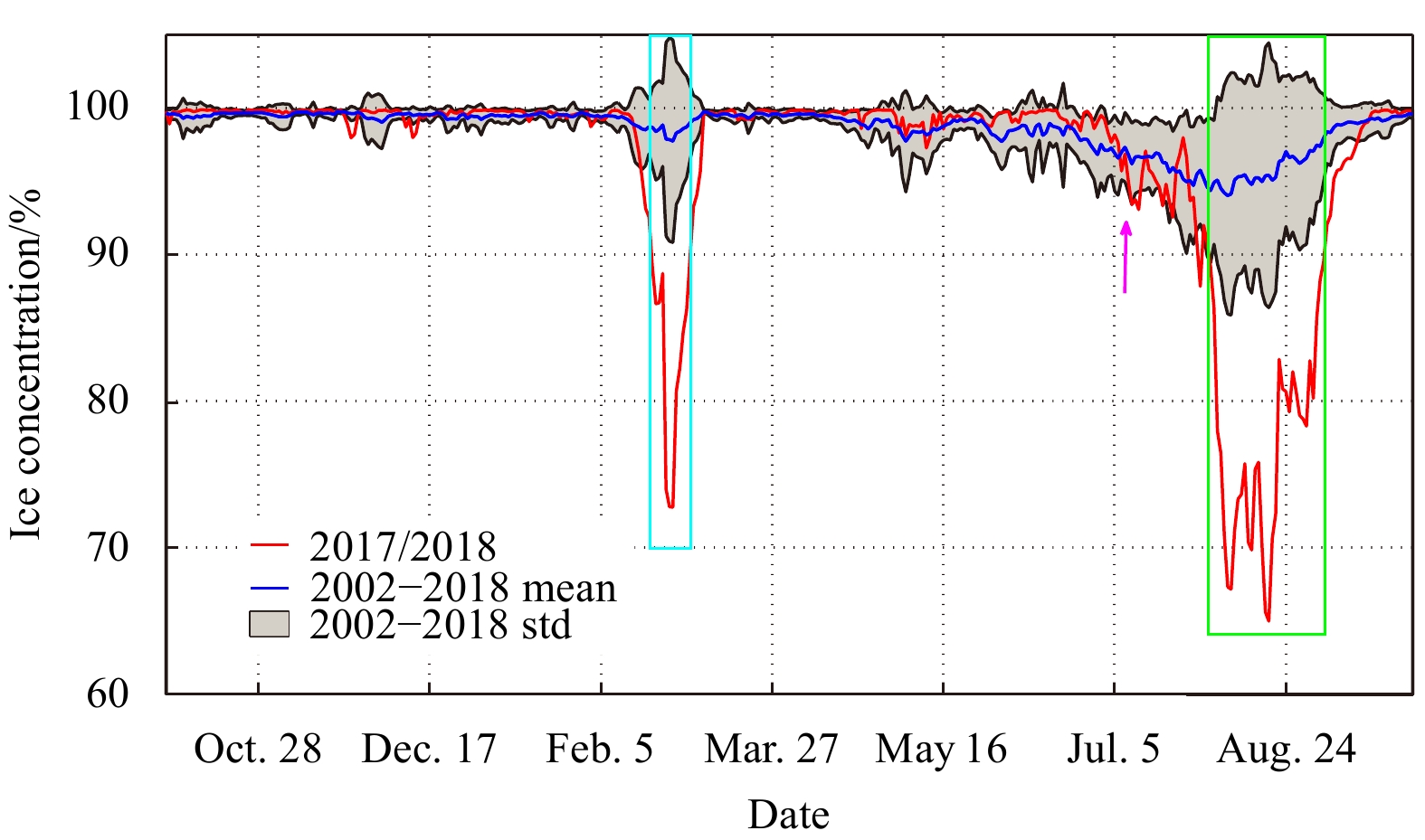
Figure 2. Spatial average ice concentration within the study region in the 2017–2018 ice season, and the multiyear average and standard deviation (2002–2018) during the same period. Cyan and green rectangles denote the periods of the polynya events. Purple arrow denotes the day on which the SLP decreased to the second lowest value during the study period.
Figure 3. Original Sentinel-1 SAR images over the study region (red block) and the sub-region (blue block) on selected days during the winter polynya event (a, b, d, f and h), and their corresponding segmented images with three ground objects of thick ice (white), thin new ice (grey), and open water (blue) (c, e, g and i).
Figure 4. Changes in sea ice concentration derived from AMSR2 and Sentinel-1 SAR observations from February 11 to March 5, 2018 within sub-region defined in Fig. 3.
Figure 5. MODIS images acquired on selected days from August 1 to September 19, 2018. Yellow denotes sea ice, blue and white depict cloud, and dark black indicates open water.
Figure 6. Time series of daily SLP gradient between 90°W and 15°E at 80°N during the 2017/2018 ice season. Also shown are the 1979–2018 climatology and its standard deviation. Cyan and green rectangles and the purple arrow denote the same events as in Fig. 2.
Figure 7. Contours of SLP and 10-m wind vectors on three selected days. The purple frame delineates the study region.
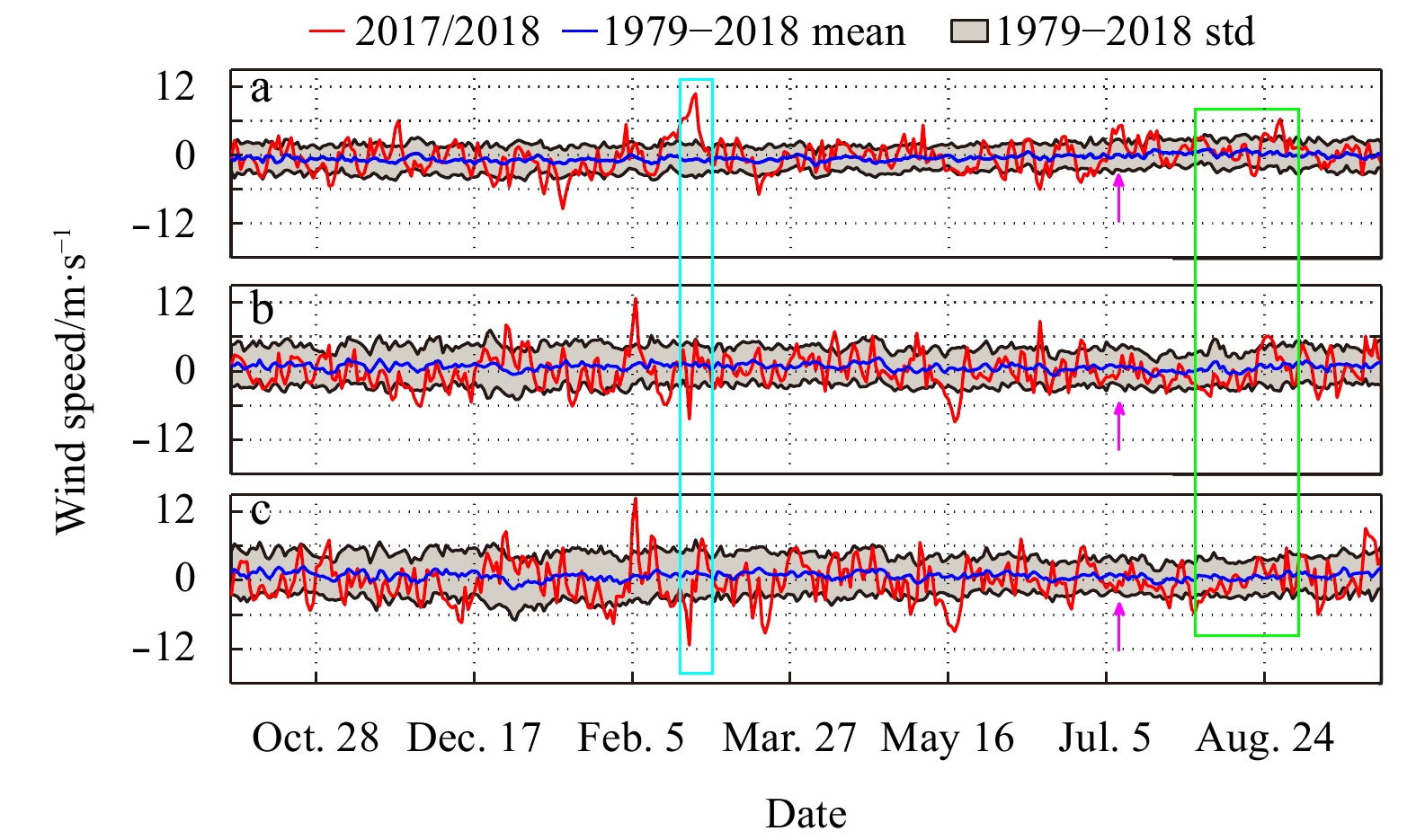
Figure 8. Meridional component of daily 10-m wind across the northern boundary of the study region (northward is positive) (a); zonal component of daily 10-m wind across the western (b) and eastern (c) boundaries (eastward is positive). Cyan and green rectangles and the purple arrow denote the same events as in Fig. 2.
Figure 9. Meridional component of daily ice motion across thenorthern boundary of the study region (northward is positive) (a); zonal component of daily ice motion across the western (b) and eastern (c) boundaries (eastward is positive). Cyan andgreen rectangles and the purple arrow denote the same events asin Fig. 2.
Figure 10. Time series of daily near-surface air temperature within the study region during the 2017/2018 ice season. Also shown are the 1979–2018 climatology and its standard deviation. Cyan and green rectangles and the purple arrow denote the same events as in Fig. 2.
Figure 11. Evolution of 500-hPa geopotential height during the formation stage of the winter polynya (a–d) and the summer polynya (e–f) in the Atlantic sector from 40°–90°N.
Figure 12. Change in the daily SLP gradient and in the difference in 500-hPa geopotential height between 90°W and 15°E at 80°N during the winter (a) and summer (b) polynya events.
Figure 13. Sentinel-1 SAR image over the Lincoln Sea and the Nares Strait on February 17, 2018 (a); and change in AMSR2 ice concentration in different blocks from north to south in February 2018 (b).


 DownLoad:


 DownLoad: