Key Laboratory of Marine Geology and Environment, Institute of Oceanology, Chinese Academy of Sciences, Qingdao 266071, China
2.
Laboratory for Marine Geology, Pilot National Laboratory for Marine Science and Technology (Qingdao), Qingdao 266237, China
3.
Center for Ocean Mega-Science, Chinese Academy of Sciences, Qingdao 266071, China
4.
University of Chinese Academy of Sciences, Beijing 100049, China
Funds:
The National Natural Science Foundation of China under contract Nos 41406215 and 41706194; a fund provided by the Qingdao National Laboratory for Marine Science and Technology; the National Natural Science Foundation of China (NSFC)-Shandong Joint Fund for Marine Science Research Centers under contract No. U1606401.
The spatial structure of the Arctic sea ice concentration (SIC) variability and the connection to atmospheric as well as radiative forcing during winter and summer for the 1979–2017 period are investigated. The interannual variability with different spatial characteristics of SIC in summer and winter is extracted using the empirical orthogonal function (EOF) analysis. The present study confirms that the atmospheric circulation has a strong influence on the SIC through both dynamic and thermodynamic processes, as the heat flux anomalies in summer are radiatively forced while those in winter contain both radiative and “circulation-induced” components. Thus, atmospheric fluctuations have an explicit and extensive influence to the SIC through complex mechanisms during both seasons. Moreover, analysis of a variety of atmospheric variables indicates that the primary mechanism about specific regional SIC patterns in Arctic marginal seas are different with special characteristics.
The Nordic seas, including the Greenland Sea, Iceland Sea, and Norwegian Sea, are of great significance in connecting the Arctic Ocean and the Atlantic Ocean. They cover an area of 2.5×10⁶ km2 in north of the Greenland-Scotland Ridge and south of the Fram Strait-Spitsbergen-North Norwegian section. The Nordic seas contain four major basins, including the Greenland Sea, Iceland Sea, Lofoten Basin, and Norwegian Basin. There is a complete mid-ocean ridge system consisting of the Kolbeinsey, Mohn and Knipovich ridges. The Jan Mayen Fracture Zone cuts through the mid-ocean ridge at the north of the Jan Mayen Island and the Vøring Plateau lies in the east of the Nordic seas. Thus, the topography features of the Nordic seas are very complicated, which greatly influence the oceanic circulation. Under the restriction of the topography, the mean circulation in each basin is cyclonic in the middle and deep layers (Voet et al., 2010).
The cold and dense water flows across the Greenland-Scotland Ridge in the southern part of the Nordic seas are termed the overflow. The overflow has three branches: the Denmark Strait overflow, the Iceland Faroe Ridge overflow, and the Faroe Bank Channel overflow from west to east. The overflow water entering the north Atlantic forms the North Atlantic deep water and bottom water because of its high density (Blindheim and Ådlandsvik, 1995; García-Ibáñez et al., 2018). The deep convection in the Greenland Sea in winter increases the density of the water mass and forms the main source of high-density water for the overflow (Hansen and Østerhus, 2000).
The high-density water flows out of the Greenland Sea across the Jan Mayen Fracture Zone and bifurcates into two parts (Hansen and Østerhus, 2000). One part flows to the south and supports the Denmark Strait overflow (Rudels et al., 2002; Harden et al., 2016). The other part flows into the Norwegian Sea via the Iceland Sea to participate in the Iceland Faroe Ridge overflow and Faroe Bank Channel overflow (Hermann, 1967; Sælen, 1990).
Observations have shown that, in the last 20 years, the total flux of the Nordic seas overflow water has remained quite stable (Quadfasel and Käse, 2007; Jochumsen et al., 2012; Karspeck et al., 2017; Østerhus et al., 2019). It has been suggested the stability of overflow must be due to a great amount of water accumulation in the Lofoten Basin, which forms the sea surface height gradient to drive the overflow and maintains the stable overflow for long periods of time (Köhl, 2010).
The characteristics of the water masses in the Lofoten Basin mainly originate from the Greenland Sea. Besides, tracer experiments (Olsen et al., 2005) have affirmed that the Greenland Sea water enters the Lofoten Basin to form the Norwegian Sea intermediate water. Observations on the dissolved oxygen also suggest that there is a close relationship between the intermediate waters in the Lofoten Basin and the Greenland Sea (Jeansson et al., 2017). However, as there is no a specific current connecting the two basins, how the Greenland Sea water enters the Norwegian Sea remains unclear.
There are two possible pathways for the export of Greenland Sea water. One is the narrow Jan Mayen Channel. Swift and Koltermann (1988) observed the current in the Jan Mayen Channel at depths ranging from 300 m to 700 m with the outflow velocity ranging from 7 cm/s to 9 cm/s. The estimated volume flux of the channel is around 0.8×10⁶ m3/s to 1.6×10⁶ m3/s (Smethie et al., 1988; Hansen and Østerhus, 2000). Shao et al. (2019) named the outflow of the Greenland Sea through the Jan Mayen Channel, the inner overflow of the Nordic seas, which was considered to generate and maintain a gigantic cold reservoir in the north part of the Norwegian Sea. However, some observation data were inconsistent with the above results. Østerhus and Gammelsrød (1999) presented evidence based on the current meter data that the current in the Jan Mayen Channel is not present all times. When the deep convection in the Greenland Sea weakened the current reversed and flowed to the Greenland Sea, which indicates that the flow in the Jan Mayen Channel might be intermittent.
The other possibility for the Greenland Sea water entering the Lofoten Basin is across the Mohn Ridge, which we termed export across the Mohn Ridge (EMR). Previous researches on the Mohn Ridge mainly focused on the features of the along-ridge current. The middle and deep circulations in the Greenland Sea and the Lofoten Basin are all cyclonic, whereas the current in the upper ocean along the western and eastern flanks of the Mohn Ridge are all flowing to the northeast. Bosse and Fer (2019) implemented some repeated measurements during two cruises of PROVOLO (water mass transformation processes and vortex dynamics in the LB of the Norwegian Sea) at a section of 150 km in length across the Mohn Ridge, and a poleward flow with the maximum speed of 0.45 m/s. Even at a depth of 1 000 m, the current speed was still 0.15 m/s. Ypma et al. (2020) also found the along-ridge current near the Mohn Ridge using the Lagrange method.
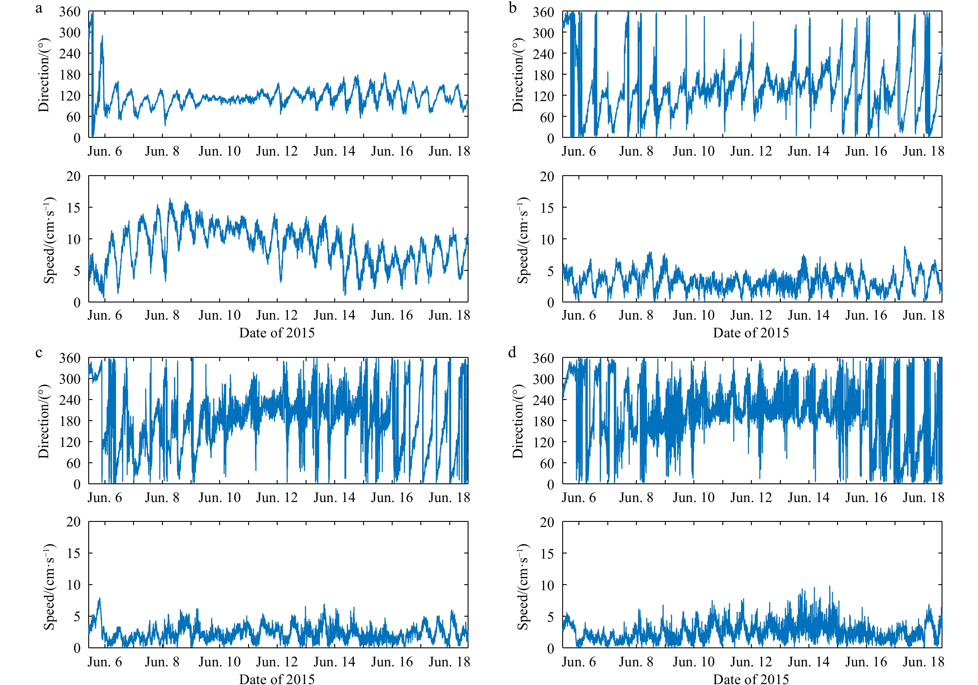
There is still little data on export over the Mohn Ridge. Some studies have reported eddies generated by instability, which would induce EMR (Blindheim, 1990; Blindheim and Rey, 2004; Budéus and Ronski, 2009). Most studies of the EMR were based on temperature and salinity data, tracer data, lowered acoustic doppler current profiler (LADCP) data, and modeling results. There have been few long-time direct current measurements for the EMR. During the joint expedition of Ocean University of China and the Akvaplan-Niva in the Nordic seas in 2015, a surface mooring with four current meters was deployed on the western flank of the Mohn Ridge (72°27'N, 0°12'E, as shown in Fig. 1). The mooring was recovered by the end of the cruise, and the data was from June 5 to June 18, 14 days in total. The main purpose of the mooring was to measure the EMR. During the cruise, three atmospheric cyclones with strong wind passed and influenced the area in which the mooring was deployed. The direct current measurement may have revealed the current features at different depths under the impact of cyclones.
Figure
1.
A sketch of the ocean circulation in the upper layer of the Nordic seas (Blindheim and Rey, 2004). The dashed lines represent the flow of Arctic-originated waters and the solid lines represent Atlantic-originated water. The pentagram (72°27'N, 0°12'E) is the location of the current meter moored in June 2015. Point A (72.75°N, 0°) and Point B (72.25°N, 1°E) at the east and west flanks of the Mohn Ridge are for calculating the air pressure difference across the Mohn Ridge through the mooring. The gray lines represent different isobaths.
In this paper, we analyzed the velocity of the EMR and connected it with the cyclone activities and mean sea level pressure variations. We estimated the annual transport of EMR based on the annual numbers of cyclones. The probable mechanism of EMR was also discussed.
2.
Data and methods
2.1
Current data
The surface mooring marked in Fig. 1, was anchored on position (72°27'N, 0°12'E) from June 5 to June 18 during the cruise in the Nordic seas in 2015. Four sets of Aanderaa Current Meter were equipped to the mooring at depths of 200 m, 500 m, 800 m, and 1 200 m. The sampling time interval was 5 min. The current data was processed using the tidal harmonic analysis, power spectrum analysis and running average to obtain the residual current. The dataset and details can be found in Section 3.
2.2
Cyclone data
The locations and characteristics dataset of the extratropical cyclone in the Northern Hemisphere from 1958 to 2016 is issued by National Snow and Ice Data Center, which is obtained by the daily sea level pressure data in the reanalysis dataset of the National Center for Environmental Prediction and the National Center for Atmospheric Research using the updated Serreze (1997) algorithm. The time interval of the data is 6 h. The cyclone data are available at http://nsidc.org/data/nsidc-0423.html.
2.3
Wind velocity data
The 10 m wind velocity in the NCEP/DOE (Department of Energy) Reanalysis 2 dataset (an improved version of the NCEP Reanalysis 1 model that fixed errors and updated parameterizations of physical processes) were used to represent the wind field variations during the observation. The spatial resolution of the data was 2.5°×2.5° and the time interval was 6 h. The wind velocity data was averaged to obtain the daily mean velocity. The NCEP data are available at https://psl.noaa.gov/data/gridded/data.ncep.reanaly-sis2.gaussian.html.
2.4
Mean sea level pressure data
The mean sea level pressure data was obtained from ERA5 hourly data (Hersbach et al., 2018) for the period from June 1, 2015 to June 30, 2015. ERA5 is the fifth generation European Centre for Medium Range Weather Forecasts reanalysis for the global climate and weather for the past 4 to 7 decades. Hourly mean sea level pressure data at 0.25° resolution was retrieved and averaged into 24-h interval. The mean sea level pressure data are available at https://cds.climate.copernicus.eu/cdsapp#!/dataset/reanalysis-era5-single-levels?tab=overview.
3.
Ocean current data analysis
The time series of raw current data are shown in Fig. 2. The current speeds at all four levels presented low frequency variations. At 200 m, the average speed was about 8.9 cm/s, which is much bigger than those at deeper three levels. At 500 m, the average speed was 3.3 cm/s; at 800 m it was 2.3 cm/s; and at 1 200 m, the average speed was 2.5 cm/s.
Figure
2.
Direction and speed of raw current data. The flow direction and speed plotted by the raw current data at the levels of 200 m (a), 500 m (b), 800 m (c), and 1 200 m (d).
The direction at the deeper three levels had remarkable high frequency variations, showing the tidal or inertial signals. However, the flow direction at 200 m did not change much, indicating stronger residual current in the upper ocean.
It was obvious that the raw current data were composed of signals with different periods, further processes were needed to remove the periodic signals and noises.
3.1
Analysis for tidal currents
The tidal harmonic analysis in the UTide Matlab toolbox offered by Codiga (2011) was applied to the raw current data. The harmonic constants are shown in Table 1. The result of harmonic analyses showed that the semidiurnal tide was dominant in this region and the diurnal tides are relatively weak.
Table
1.
Tidal current harmonic constants
Depth/m
Constituent
Zonal component
Meridional component
H/(cm·s−1)
g/(º)
H/(cm·s−1)
g/(º)
200
O1
0.54
206
0.31
347
K1
0.24
270
0.80
277
M2
1.94
56
2.46
328
500
O1
0.27
222
0.33
293
K1
0.57
267
0.73
252
M2
0.78
236
0.38
92
800
O1
0.29
199
0.29
318
K1
0.40
258
0.75
272
M2
0.24
345
0.68
336
1 200
O1
0.19
239
0.24
347
K1
0.31
266
0.82
265
M2
0.76
202
1.07
67
Note: H denotes the amplitude of flow rate; g denotes phase lag.
The zonal components and meridional components were composed to obtain the tidal current. The velocity of tidal current at each level was weak compared to the total current. At 200 m, the average tidal current speed was 2.34 cm/s; at 500 m, it was about 0.87 cm/s; at 800 m, it was about 0.68 cm/s; and at 1 200 m, the average speed was 1.05 cm/s. Therefore, the tidal current had little impact on residual currents near the Mohn Ridge.
3.2
Filtering of the inertial and high frequency components
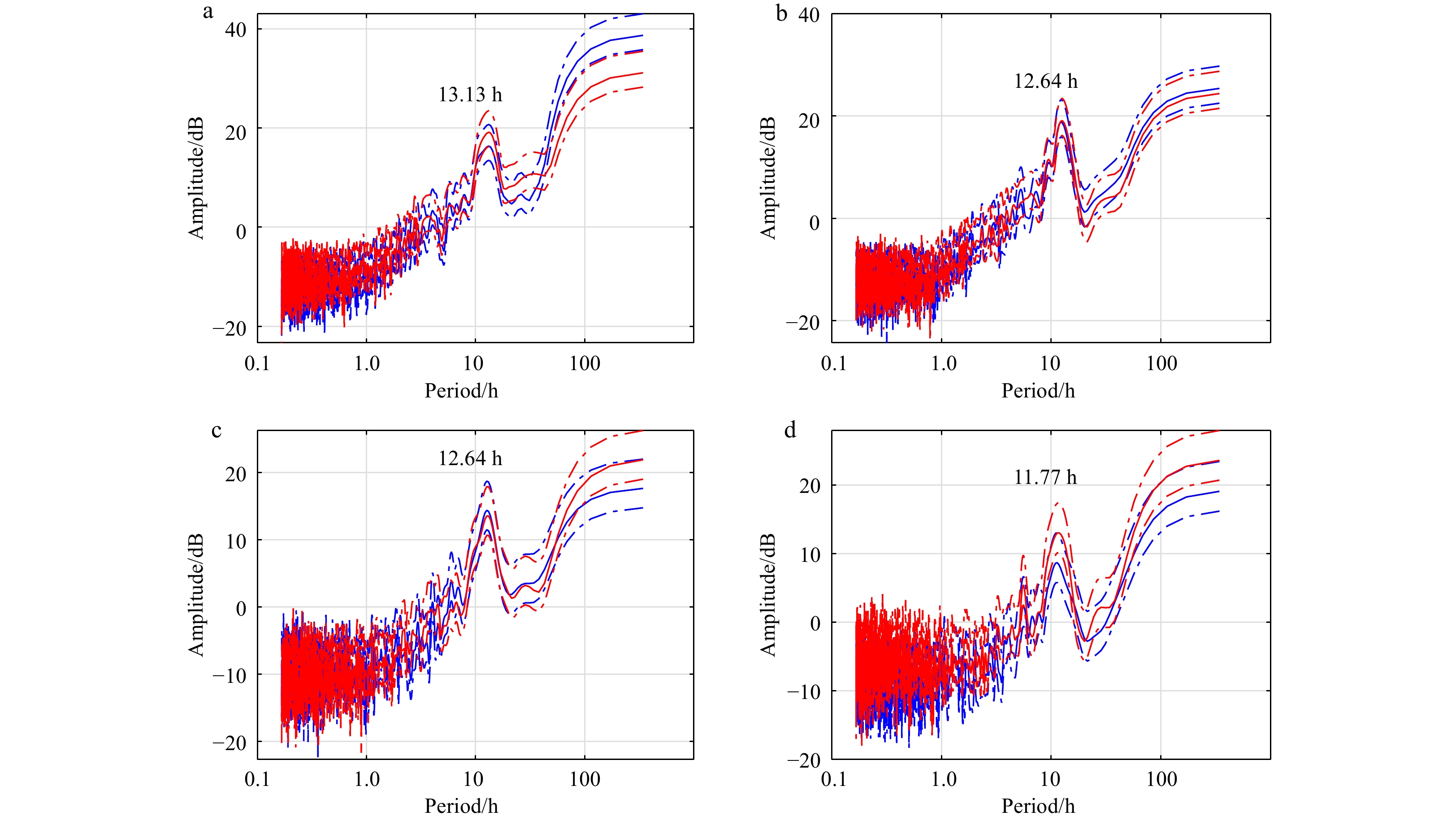
After subtracting the tidal currents from the raw data, there were still some high frequency variations, inertial currents and low-frequency residual components. Taking the power spectrum analyses, the dominant periods at 200 m, 500 m, 800 m, and 1 200 m were 13.13 h, 12.64 h, 12.64 h, and 11.77 h, respectively (Fig. 3). The dominant signals were expected to be the inertial currents, as the theoretical period of inertial current at this latitude was 12.55 h. The differences were mainly due to the confusion between the semidiurnal tides and the inertial currents because their periods were quite close.
Figure
3.
Power spectral density with 95% confidence bounds after removing the tidal current at 200 m (a), 500 m (b), 800 m (c), and 1 200 m (d). The blue lines represent the east component, and the red lines represent the north component.
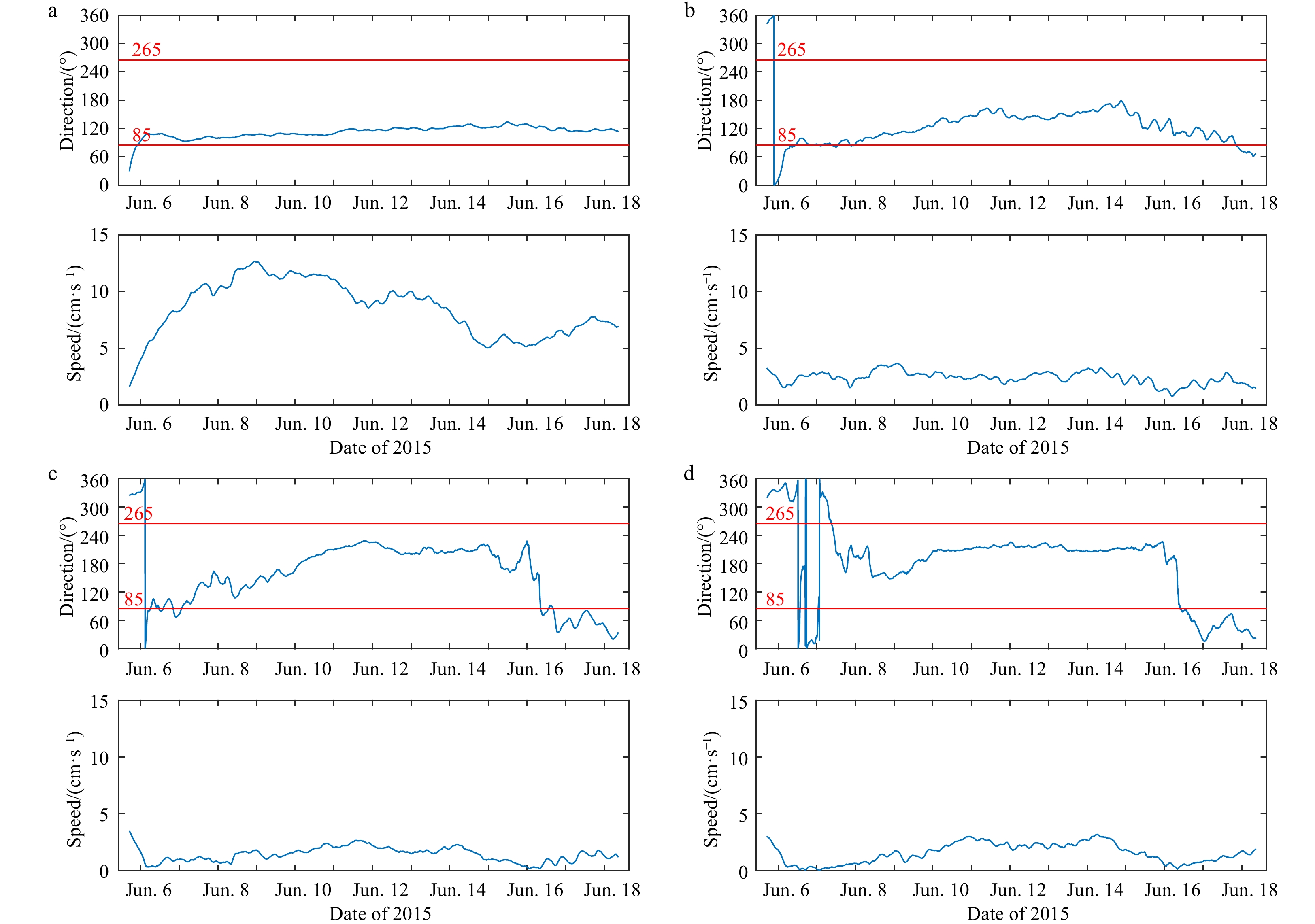
The running average method was used for filtering the inertial current and the high frequency signals. The time window was selected as 13.25 h that is longer than inertial period, i.e., 159 points for sampling interval of 5 min. The running average was separately applied to the east and north components, and the components of the residual current were obtained. By synthesizing the residual components, the direction and speed of the low frequency flow are shown in Fig. 4.
Figure
4.
Variations of residual current direction and speed at the four levels: 200 m (a), 500 m (b), 800 m (c), and 1 200 m (d). The red lines represent the inclination of the Mohn Ridge.
In Fig. 4, the 85° and 285° are the rough direction of the Mohn Ridge, and the flow appeared between the red lines represents the water transportation from the Greenland Sea to the Lofoten Basin, which is also called EMR.
4.
EMR related to atmospheric forcing
4.1
Wind variation during observation
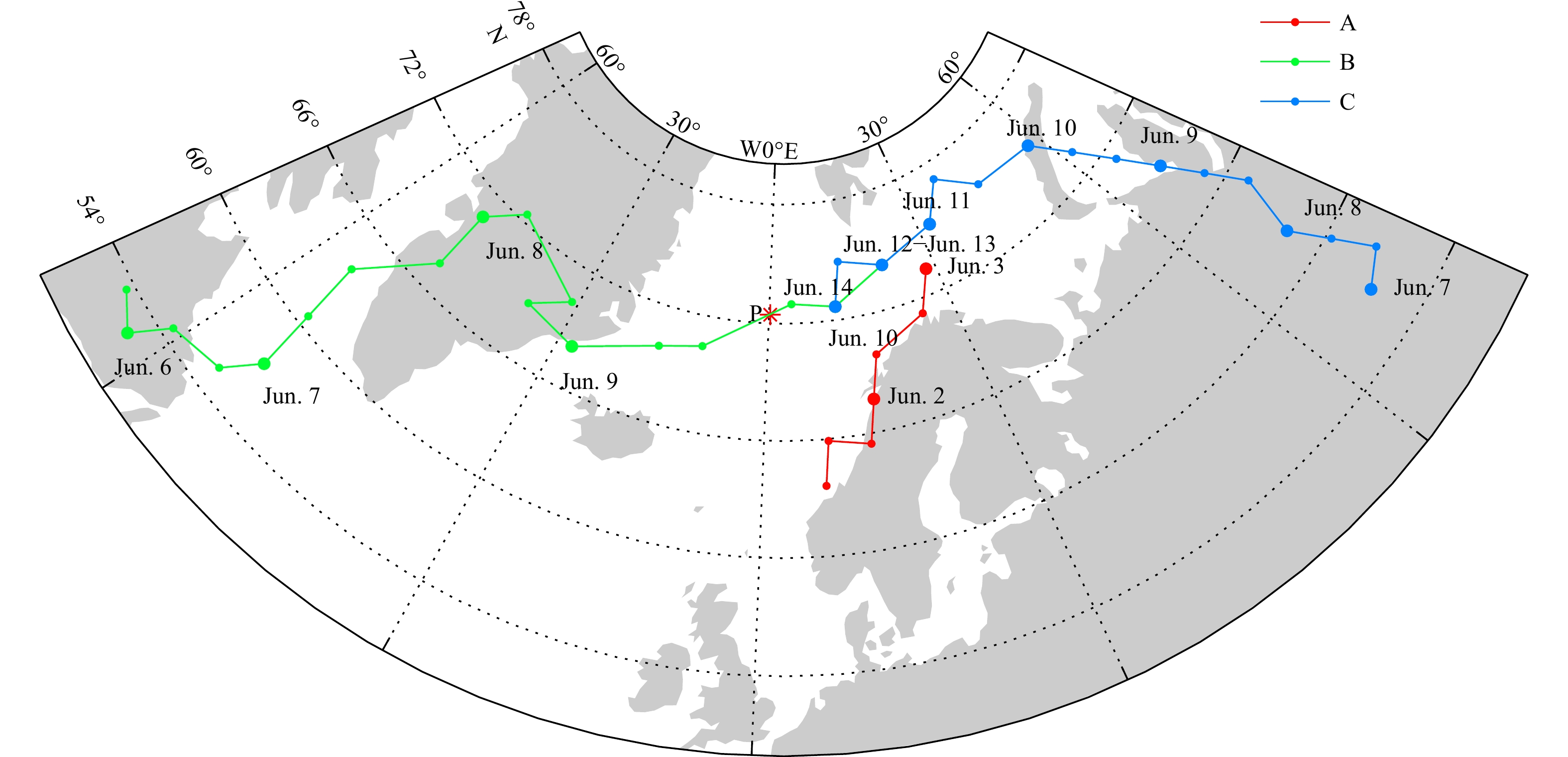
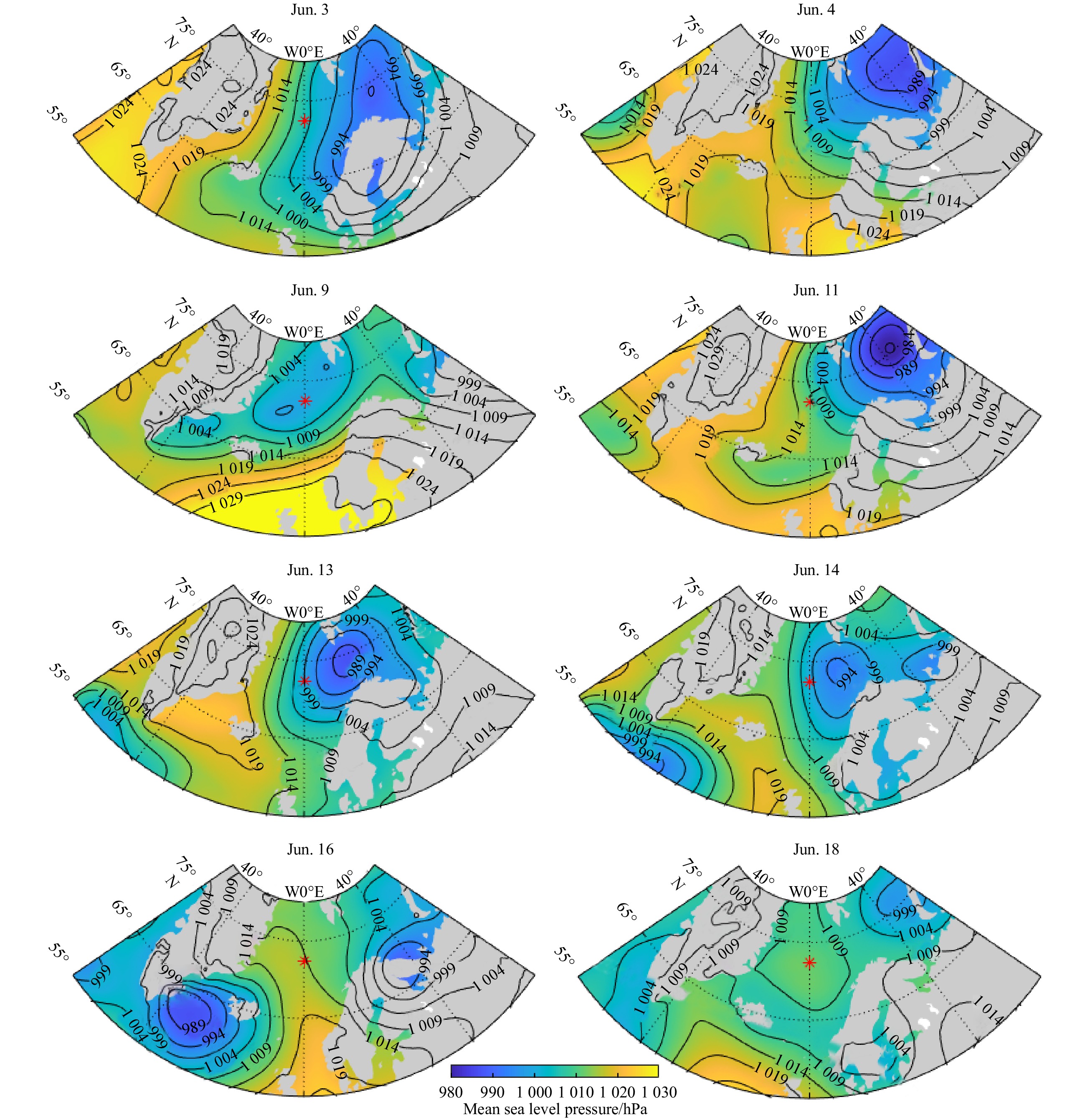
Combining the cyclone data with the NCEP reanalysis wind velocity data, three cyclones were identified that passed the region (70–75°N, 20°W–15°E) adjacent to the buoy, greatly affecting the regional wind field. The cyclones are numbered 2823 (Cyclone A), 2899 (Cyclone B), and 2915 (Cyclone C) and their trajectories are shown in Fig. 5.
Figure
5.
Trajectories of three cyclones. The asterisk represents the location of the surface mooring. Dots represent the center of the cyclone and the dates are marked near the dots.
Cyclone A passed the region from June 1 to June 3, and its influence on the flow field still affected the current velocity on June 5 when the mooring was deployed. Cyclone B appeared from June 5 to June 10, and greatly influenced the records of the current meter. As it moved to the north, the central pressure decreased from 1 008 hPa to 992 hPa, and then rose to 997 hPa. Cyclone C entered the Kara Sea on June 9 and then moved southwesterly and swept the northern Nordic seas until June 15. The central pressure of Cyclone C decreased to 980 hPa before rising to 997 hPa then. These three cyclones passed through the Nordic seas successively, causing strong wind and altered ocean currents.
The 10 m wind velocity data in the NCEP-DOE reanalysis dataset are used to present the wind field variations during the observation.
As we can see from Fig. 6, the wind field was a superposition of the winter northerly wind and the cyclonic wind field. On June 3 and June 4, Cyclone A had already disappeared and north wind prevailed in the Nordic seas. From June 7 the wind field became cyclonic and the wind at the mooring location was from the south because Cyclone B moved to the north, moving to the east of Greenland Island. After that, Cyclone B gradually moved away from the mooring and the wind field returned to the northerly wind on June 11 and June 12. Beginning on June 13, Cyclone C approached the mooring and the northerly wind prevailed in the Nordic seas. The center of the Cyclone C approached the mooring location on June 14 and moved away on June 16. From June 17 to June 20, the wind calmed.
Figure
6.
Daily mean wind field during observation. The red asterisk represents the moored location, and date of each subplot is marked at the top.
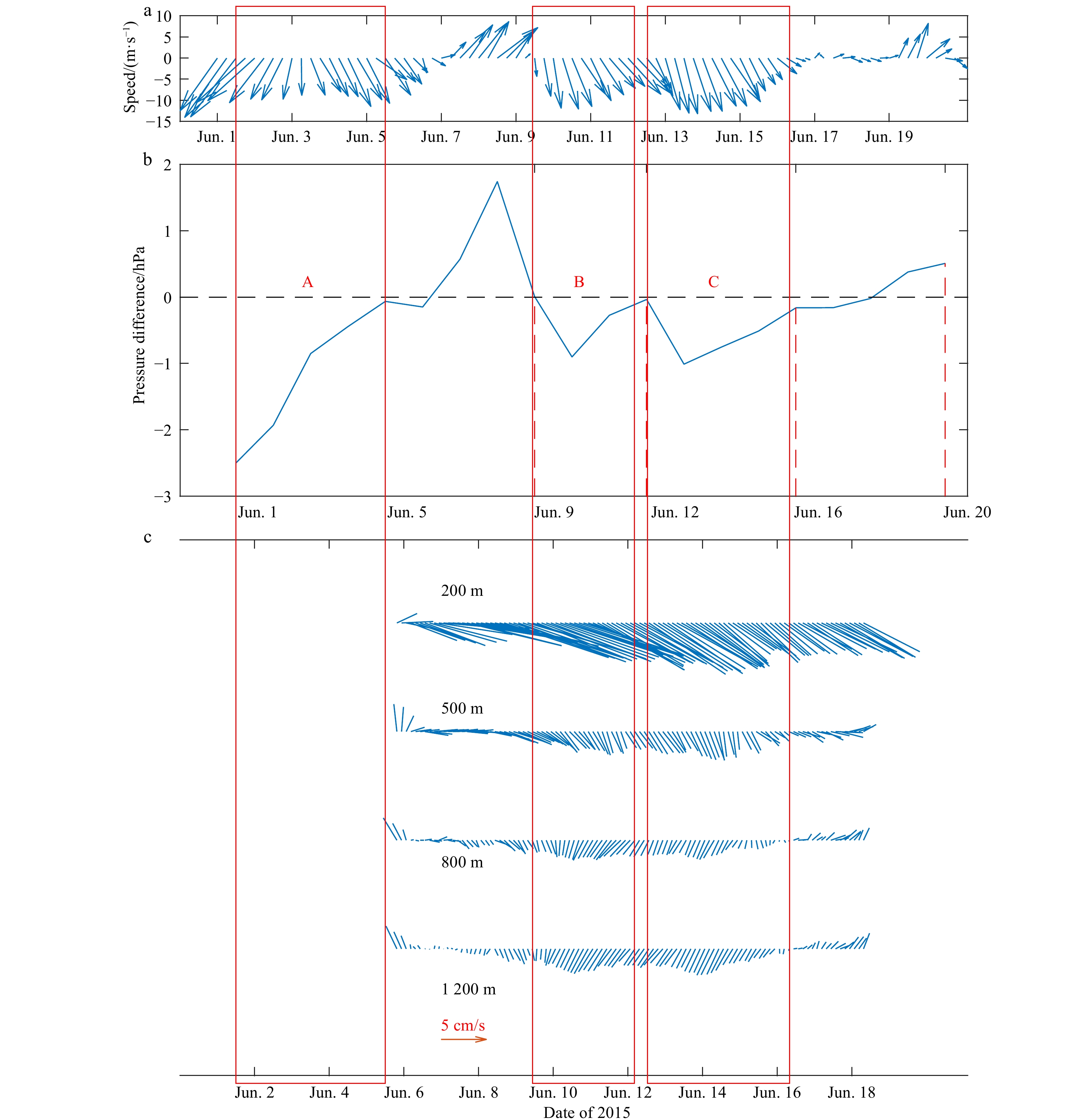
The influence of the mean sea level pressure (SLP) on residual current was also studied. The differences of air pressure across the Mohn Ridge at the mooring site were obtained by subtracting SLP of Point A (72.75°N, 0°) from that of Point B (72.25°N, 1°E). The temporal variation of wind vectors, differences of SLP and residual current vectors were shown in Fig. 7.
Figure
7.
Wind vector 10 m above the sea surface (a), the mean sea surface pressure variations between A and B (b) and vector diagram of residual current at each level (c). The rectangle represents the period of each cyclone.
As shown in Fig. 7a, the northerly wind was dominated by Cyclone A from June 1 to June 7. After June 7, the local wind changed to a southwest wind and wind speed continued to increase until June 9, indicating the transit trajectory of Cyclone B along the west of the surface mooring. Since June 9, the wind changed again to the northwest until June 16, showing the trajectory of Cyclone C east of the mooring. From June 15 to June 19, the local wind gradually turned to the west and southwest from northwest and wind speed decreased quickly.
The initial direction of the residual current at 200 m was 30° from June 5 to June 6 under the impact of Cyclone A (Fig. 7c), indicating that Greenland Sea water had not entered the Lofoten Basin. After June 6, the flow direction at 200 m depth was quite stable from 100° to 130°, showing an outflow from the Greenland Sea into the Lofoten Basin. Cyclone B came from the southeast Nordic seas since June 8, and the maximum current speed of 0.12 m/s appeared on June 9. Cyclone C began to influence the observation area on June 12 and the maximum speed appeared on June 13. After June 15, the speed and direction of the flow at 200 m changed little. For most of the observation period the direction of the outflow at 200 m was southeast, which brought the Greenland Sea water into the Lofoten Basin.
Current variations at 500 m, 800 m, and 1 200 m are shown in Fig. 7. Under the influence of Cyclone A, the direction of the residual current at 500 m and 800 m changed from northwest to about 90°, while it changed to around 220° at 1 200 m. Under the consecutive influence of Cyclones B and C, the residual current at each level flowed southeastward or southwestward, around 148° at 500 m, 205° at 800 m and 213° at 1 200 m. When Cyclone C disappeared, the direction of the deeper three levels rapidly recovered to around 60° and the export across the Mohn Ridge suspended.
The local wind variations and residual current variations match well with the variations of difference of the mean SLP. As presented in Fig. 7b, the minimum of SLP differences appeared when the cyclones passed the mooring site. The negative SLP differences drove the EMR from the Greenland Sea. The matching of cyclones and the SLP differences also indicated that the outflow from the Greenland Sea to Lofoten Basin was arisen by driving of cyclones, not by free eddies generated by instability processes.
The negative SLP difference implies the anomalous SLP field as shown in Fig. 8. When a cyclone passed the Nordic seas, a low-pressure center associated with the cyclone will appear, which sometimes overwhelms the Icelandic Low, and moves to the east part of the Nordic seas. The low-pressure center appeared in the northeast of the mooring location on June 3. Then, it continuously moved to the north on June 4 and gradually disappeared. On June 9, the low-pressure center covered the mooring location. From June 11 to June 14, the low-pressure center moved close to observation location from northeast to southwest. On June 16, there were two low-pressure centers on the map, one was the Icelandic Low in the south and the other is a low pressure induced by a cyclone in the north, both were far from the mooring.
We believed that the cross-ridge SLP difference dominated the geostrophic current along the ridge in the situation without cyclones. When a cyclone passing, the low air pressure interfered the SLP difference and produced the geostrophic deviation, which allowed the Greenland Sea water to flow outward. So, the variation of SLP difference was the key factor to influence the deep current.
4.3
Discussion of export across the Mohn Ridge
Based on water mass analysis, there are huge amounts of water entering the Lofoten Basin (Blindheim,1990), but the mechanism of the export is still unclear because there is no direct current connecting the two basins. Figure 7 shows that during the last few days of the observation, the cyclones disappeared and the current direction at the deeper three levels returned to northeastward (around 60°). This suggested that the current flows northeastward along the ridge without the influence of cyclones, consistent with the mean circulation pattern (shown in Fig. 1). The topography-constrained current obstructed the Greenland Sea water from crossing the Mohn Ridge and entering the Lofoten Basin. However, the current at 200 m was an exception, which still flowed southward at that time, being inconsistent with the northeastward flow at the deeper levels. More observations are needed to reveal the reason for the quasi-opposite flow at 200 m.
From June 9 to June 15, the transit cyclones altered the current direction to southeastward at all depths, which allowed the Greenland Sea water to enter the Lofoten Basin. Therefore, the major driving mechanism for the EMR might be passing cyclones, with which the outflow of the Greenland Sea water should be intermittent.
It was pointed out in previous investigations that the current along the Mohn Ridge could cause instability and produce eddies, which would lead to water transport across the Mohn Ridge (Blindheim, 1990; Blindheim and Rey, 2004; Budéus and Ronski, 2009). The current embodied a quite steady outflow in both speed and direction from June 9 to June 15. It did not show the alternating flow field of a passing eddy, so we considered that the outflow was not caused by a free eddy. However, a stationary vortex could show such a quite steady outflow, which is impossible to be detected with only one mooring, if any.
Our result suggested that the EMR was caused by the abnormal sea surface height field induced by the cyclones. Under normal circumstances, the sea surface height is high at the rim and low at the center of the Greenland Sea, and the pressure gradient force is pointed toward the Greenland Sea, which matches the cyclonic circulation in the Greenland Sea (Fig. 1). The wind field also supports the current at both flanks of the Mohn Ridge flowing to the northeast. When the cyclones were passing, the central low pressure of the cyclones disturbed the sea surface height field intensely and the sea level decreased causing a regional pressure gradient force pointing to outside the Greenland Sea. The outward pressure gradient force destroyed the geostrophic current at all depths, and drove the outward flow as presented in Fig. 7.
4.4
Estimation of volume transport of EMR
The volume transport is very important because it decides the scale of the cool pool in the northern Nordic seas, the possible Norwegian Sea branch of the Greenland-Scotland Ridge overflow, and the northward flux of the cold recirculation along the Norwegian coast under the Atlantic water. It is difficult to estimate the volume flux of EMR from the Greenland Sea using only a single mooring and a short-term measurement. However, it is still possible to roughly estimate the volume flux of the intermittent outflow due to the cyclonic storms if we know the velocity of the residual current and the number of this kind of cyclone per year.
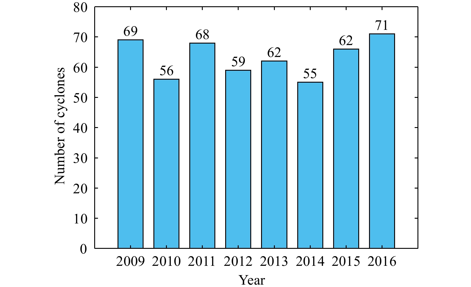
According to the results in Fig. 4, the conservative estimate of the mean value of the velocity component that is perpendicular to the Mohn Ridge is 1.1 cm/s. Assuming that a passing cyclone from south to north will influence consecutively the outflow in the same way along the Mohn Ridge of 550 km length, and considering that the outflow appeared in the top 1 200 m, the mean flux of the outflow is about 7.3 ×10⁶ m3/s when the cyclone is passing and outflow occurs. According to the results in this study, water transport caused by a cyclone continued for about 3 days. The total number of cyclones appearing near the Mohn Ridge (70°–75°N, 20°W–15°E) from 2009 to 2016 is plotted in Fig. 9 and the multiyear averaged cyclone number is 63. Therefore, the annual mean transport flux of EMR is estimated about 3.8×10⁶ m3/s. The estimation value is rather rough, because the speed might be larger or smaller, the outflow may appear deeper than 1 200 m, and the influence scope of a cyclone might be shorter than the length of the Mohn Ridge.
Figure
9.
Number of cyclones near the Mohn Ridge from 2009 to 2016.
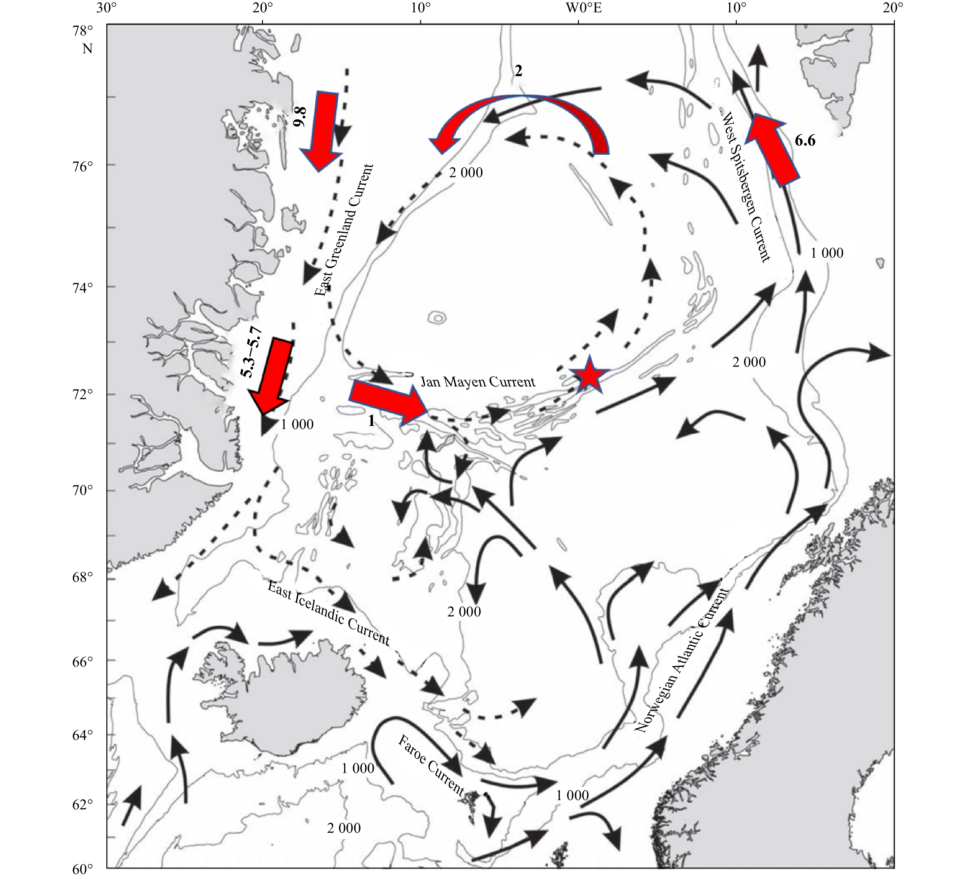
Based on the volume conservation in the Greenland Sea, the volume flux of EMR can be estimated by the water flux at the other four passages (Fig. 10). The estimation for the water fluxes in these pathways are listed in Table 2. The values obtained by previous researchers were quite different, which might have been caused by seasonal anomalies, interannual deviation, or low-frequency oscillation. The estimated values of the flux through Fram Strait are over a large range, 5.8×10⁶ m3/s to 13.0×10⁶ m3/s. As the difference might include the interannual information, it is reasonable to estimated it as 9.8×10⁶ m3/s by the mean of the six values shown in Table 2. The inflow from the recirculated Atlantic water is about 2×10⁶ m3/s; the outflow over the Jan Mayen Fracture Zone is about 5.3×10⁶ m3/s to 5.7×10⁶ m3/s; and the outflow from the Jan Mayen Channel is about 1×10⁶ m3/s. Thus, the flux of the EMR should be about 5.1×10⁶ m3/s to 5.5×10⁶ m3/s. Our result is smaller than the estimation based on volume conservation.
Figure
10.
Water fluxes (unit: Sv) of each passage in the Greenland Sea.
The estimated values based on our measurement or by volume conservation may be inaccurate due to the short time span of our observations and the striking differences from previous studies. The flux of the EMR might vary with time with the varying wind, the changing convection in the Greenland Sea, and the large-scale adjustment of both the Arctic and Atlantic oceans. The volume flux of EMR driven by passing cyclones might not the only mechanism by which the Greenland Sea water enters the Lofoten Basin. More studies are necessary to reveal the mechanism of EMR and accurately determine the flux through this important pathway.
We connected the Greenland Sea outflow with the cyclone movements by analyzing the current data. Cyclone activity may destroy the geostrophic current restriction, intermittently causing Greenland Sea water to enter the Lofoten Basin. A specific mechanism was given for water transport across the Mohn Ridge, which helps us understand the features and patterns of Greenland Sea water export.
5.
Conclusions
In the Nordic seas, the Mohn Ridge is a part of a middle-ridge system that separates the Greenland Sea and Lofoten Basin. The outflow across the Mohn Ridge from the Greenland Sea might be an important contribution to the Greenland-Scotland Ridge overflow to the North Atlantic Ocean. Previous studies support the existence of EMR through water mass analysis, chemical and numerical tracing, vessel-based acoustic doppler current profiler (ADCP) measurements and LADCP casting. Since there is no obvious current connecting the two basins, the manner of the export from the Greenland Sea is still unclear. Also, since there is no direct current measurement, the water transportation flux remains unclear. During a cruise in the Nordic seas in 2015, a surface mooring was deployed on the Mohn Ridge (72°27'N, 0°12'E,) on June 5, and recovered by the end of the cruise at June 18. The mooring equipped four Andre current meters at depths of 200 m, 500 m, 800 m, and 1 200 m. During the cruise, three cyclones passed by the Northern Nordic seas. The data revealed the influence of cyclone activity on the EMR. By removing the tidal signal with harmonic analysis and filtering the inertial and high frequency signals with running average, the residual current was obtained.
In the absence of cyclones, the Greenland Sea circulation is cyclonic, and on the west flank of the Mohn Ridge the flow is northeastward (around 60°), which constrains the Greenland Sea water from entering the Lofoten Basin. When the cyclones appeared in the area adjacent to the mooring, currents at all depths flowed to the south or southeast, indicating the occurrence of the EMR, with which the Greenland Sea water was transported to the Lofoten Basin. When the cyclones left, the currents in the deeper three levels quickly recovered and turned to the northeast. Our result suggests that the Greenland Sea water outflow is intermittent and only occurs during cyclone activities.
Previous studies suggested that the eddies generated by the instability of the current along the Mohn Ridge could induce transport across the Mohn Ridge. According to our result, however, the southward currents during cyclone passing are quite steady in speed and direction, indicating cyclone-induced intermittent flow, not moving eddies or stationary vortexes.
The probable mechanism for EMR is discussed in this paper. Without cyclones, the wind-driven sea level height of the Greenland Sea is higher at the margin and lower at the center, with the pressure gradient force pointed towards the interior of the Greenland Sea. The low pressure of cyclones wiped out the column with higher pressure and caused a pressure gradient force from the Greenland Sea to the outside to drive the EMR.
SSH was the driven factor of deep current, which was built by the cyclonic wind field. Because wind include wind direction information, we select to build the connection of EMR with wind in this study for better understanding of EMR.
Although the outflow induced by cyclones is intermittent, the annual mean of the volume flux of EMR is expectable. It was difficult to estimate the flux of EMR using only a single mooring and short-term measurement data. In this study, we roughly estimated the volume flux of the intermittent outflow based on the residual current results and the annual mean cyclone number. The annual mean flux of EMR was estimated to be about 3.8×10⁶ m3/s, which was a bit smaller than the estimation based on volume conservation.
The results indicated an important mechanism through which the Greenland Sea water is transported to the Lofoten Basin. As extratropical cyclones occur frequently in the Nordic seas, the contribution of cyclonic storms to EMR is of great importance for the water balance in the Nordic seas, which potentially influences the global thermohaline circulation through the Greenland-Scotland overflow.
Årthun M, Eldevik T, Smedsrud L H, et al. 2012. Quantifying the influence of Atlantic heat on Barents Sea ice variability and retreat. Journal of Climate, 25(13): 4736–4743. doi: 10.1175/JCLI-D-11-00466.1
[2]
Bamber J L, Tedstone A J, King M D, et al. 2018. Land ice freshwater budget of the Arctic and North Atlantic Oceans: 1. Data, methods, and results. Journal of Geophysical Research: Oceans, 123(3): 1827–1837. doi: 10.1002/2017JC013605
[3]
Bi Haibo, Sun Ke, Zhou Xuan, et al. 2016. Arctic Sea ice area export through the fram strait estimated from satellite-based data: 1988–2012. IEEE Journal of Selected Topics in Applied Earth Observations and Remote Sensing, 9(7): 3144–3157. doi: 10.1109/JSTARS.2016.2584539
[4]
Boisvert L N, Petty A A, Stroeve J C. 2016. The impact of the extreme winter 2015/16 Arctic cyclone on the Barents–Kara Seas. Monthly Weather Review, 144(11): 4279–4287. doi: 10.1175/MWR-D-16-0234.1
[5]
Comiso J C. 2006. Abrupt decline in the Arctic winter sea ice cover. Geophysical Research Letters, 33(18): L18504
[6]
Comiso J C. 2017. Bootstrap Sea Ice Concentrations from Nimbus-7 SMMR and DMSP SSM/I-SSMIS, Version 3. [1979–2017]. Boulder, Colorado USA: NASA National Snow and Ice Data Center Distributed Active Archive Center, doi: https://doi.org/10.5067/7Q8HCCWS4I0R.[2018.04.03]
[7]
Comiso J C, Hall D K. 2014. Climate trends in the Arctic as observed from space. Wiley Interdisciplinary Reviews: Climate Change, 5(3): 389–409. doi: 10.1002/wcc.277
[8]
Comiso J C, Parkinson C L, Gersten R, et al. 2008. Accelerated decline in the Arctic Sea ice cover. Geophysical Research Letters, 35(1): L01703
[9]
Crasemann B, Handorf D, Jaiser R, et al. 2017. Can preferred atmospheric circulation patterns over the North-Atlantic-Eurasian region be associated with arctic sea ice loss?. Polar Science, 14: 9–20. doi: 10.1016/j.polar.2017.09.002
[10]
Curry J A, Schramm J L, Serreze M C, et al. 1995. Water vapor feedback over the Arctic Ocean. Journal of Geophysical Research: Atmospheres, 100(D7): 14223–14229. doi: 10.1029/95JD00824
[11]
Deser C, Teng Haiyan. 2008. Evolution of Arctic sea ice concentration trends and the role of atmospheric circulation forcing, 1979–2007. Geophysical Research Letters, 35(2): L02504
[12]
Deser C, Walsh J E, Timlin M S. 2000. Arctic sea ice variability in the context of recent atmospheric circulation trends. Journal of Climate, 13(3): 617–633. doi: 10.1175/1520-0442(2000)013<0617:ASIVIT>2.0.CO;2
[13]
Ding Qinghua, Schweiger A J B, L’heureux M L, et al. 2016. Influence of the recent high-latitude atmospheric circulation change on summertime Arctic sea ice. Nature Climate Change, 7(4): 289–295
[14]
Eisen O, Kottmeier C. 2000. On the importance of leads in sea ice to the energy balance and ice formation in the Weddell Sea. Journal of Geophysical Research: Oceans, 105(C6): 14045–14060. doi: 10.1029/2000JC900050
[15]
Fan Tingting, Huang Fei, Su Jie. 2012. The seasonal March of dominate mode of the mid-high latitude atmosphere circulation in northern hemisphere and the associated Arctic sea ice. Periodical of Ocean University of China (in Chinese), 42(7): 19–25
[16]
Fang Zhifang, Wallace J M. 1994. Arctic sea ice variability on a timescale of weeks and its relation to atmospheric forcing. Journal of Climate, 7(12): 1897–1914. doi: 10.1175/1520-0442(1994)007<1897:ASIVOA>2.0.CO;2
[17]
Germe A, Houssais M N, Herbaut C. 2011. Greenland Sea sea ice variability over 1979–2007 and its link to the surface atmosphere. Journal of Geophysical Research: Oceans, 116(C10): C10034. doi: 10.1029/2011JC006960
Hegyi B M, Taylor P C. 2017. The regional influence of the Arctic Oscillation and Arctic Dipole on the wintertime Arctic surface radiation budget and sea ice growth. Geophysical Research Letters, 44(9): 4341–4350. doi: 10.1002/2017GL073281
[20]
Hegyi B M, Taylor P C. 2018. The unprecedented 2016–2017 Arctic sea ice growth season: the crucial role of atmospheric rivers and longwave fluxes. Geophysical Research Letters, 45(10): 5204–5212. doi: 10.1029/2017GL076717
[21]
Herbaut C, Houssais M N, Close S, et al. 2015. Two wind-driven modes of winter sea ice variability in the Barents Sea. Deep Sea Research Part I: Oceanographic Research Papers, 106: 97–115. doi: 10.1016/j.dsr.2015.10.005
[22]
Hinzman L D, Bettez N D, Bolton W R, et al. 2005. Evidence and implications of recent climate change in northern Alaska and other Arctic Regions. Climatic Change, 72(3): 251–298. doi: 10.1007/s10584-005-5352-2
[23]
Johannessen O M, Bengtsson L, Miles M W, et al. 2004. Arctic climate change: observed and modelled temperature and sea-ice variability. Tellus A, 56(4): 328–341. doi: 10.3402/tellusa.v56i4.14418
[24]
King M P, Hell M, Keenlyside N. 2016. Investigation of the atmospheric mechanisms related to the autumn sea ice and winter circulation link in the northern Hemisphere. Climate Dynamics, 46(3–4): 1185–1195
[25]
Kwok R. 2009. Outflow of Arctic Ocean sea ice into the Greenland and Barents Seas: 1979–2007. Journal of Climate, 22(9): 2438–2457. doi: 10.1175/2008JCLI2819.1
[26]
Lee S, Gong Tingting, Feldstein S B, et al. 2017. Revisiting the cause of the 1989–2009 Arctic surface warming using the surface energy budget: downward infrared radiation dominates the surface fluxes. Geophysical Research Letters, 44(20): 10654–10661. doi: 10.1002/2017GL075375
[27]
Lei Ruibo, Gui Dawei, Hutchings J K, et al. 2019. Backward and forward drift trajectories of sea ice in the northwestern Arctic Ocean in response to changing atmospheric circulation. International Journal of Climatology, 39(11): 4372–4391. doi: 10.1002/joc.6080
[28]
Letterly A, Key J, Liu Yinghui. 2016. The influence of winter cloud on summer sea ice in the Arctic, 1983–2013. Journal of Geophysical Research: Atmospheres, 121(5): 2178–2187. doi: 10.1002/2015JD024316
[29]
Lindsay R, Schweiger A. 2015. Arctic sea ice thickness loss determined using subsurface, aircraft, and satellite observations. The Cryosphere, 9(9): 269–283
[30]
Liu Yinghui, Key J R. 2014. Less winter cloud aids summer 2013 Arctic sea ice return from 2012 minimum. Environmental Research Letters, 9(4): 044002. doi: 10.1088/1748-9326/9/4/044002
[31]
Liu Zheng, Schweiger A. 2017. Synoptic conditions, clouds, and sea ice melt onset in the Beaufort and Chukchi seasonal ice zone. Journal of Climate, 30(17): 6999–7016. doi: 10.1175/JCLI-D-16-0887.1
[32]
Lynch A H, Serreze M C, Cassano E N, et al. 2016. Linkages between Arctic summer circulation regimes and regional sea ice anomalies. Journal of Geophysical Research: Atmospheres, 121(13): 7868–7880. doi: 10.1002/2016JD025164
[33]
Markus T, Stroeve J C, Miller J. 2009. Recent changes in Arctic sea ice melt onset, freezeup, and melt season length. Journal of Geophysical Research: Oceans, 114(C12): C12024. doi: 10.1029/2009JC005436
[34]
Maslanik J A, Fowler C, Stroeve J, et al. 2007. A younger, thinner Arctic ice cover: Increased potential for rapid, extensive sea-ice loss. Geophysical Research Letters, 34(24): L24501. doi: 10.1029/2007GL032043
[35]
Maslanik J, Stroeve J, Fowler C, et al. 2011. Distribution and trends in Arctic sea ice age through spring 2011. Geophysical Research Letters, 38(13): L13502
[36]
Nakanowatari T, Inoue J, Sato K, et al. 2015. Summertime atmosphere–ocean preconditionings for the Bering Sea ice retreat and the following severe winters in North America. Environmental Research Letters, 10(9): 094023. doi: 10.1088/1748-9326/10/9/094023
[37]
Nghiem S V, Rigor I G, Perovich D K, et al. 2007. Rapid reduction of Arctic perennial sea ice. Geophysical Research Letters, 34(19): L19504. doi: 10.1029/2007GL031138
[38]
Ogi M, Rigor I G, McPhee M G, et al. 2008. Summer retreat of Arctic sea ice: role of summer winds. Geophysical Research Letters, 35(24): L24701. doi: 10.1029/2008GL035672
[39]
Ogi M, Rysgaard S, Barber D G. 2016. Importance of combined winter and summer Arctic Oscillation (AO) on September sea ice extent. Environmental Research Letters, 11(3): 034019. doi: 10.1088/1748-9326/11/3/034019
[40]
Ogi M, Wallace J M. 2007. Summer minimum Arctic sea ice extent and the associated summer atmospheric circulation. Geophysical Research Letters, 34(12): L12705. doi: 10.1029/2007GL029897
[41]
Ogi M, Yamazaki K, Wallace J M. 2010. Influence of winter and summer surface wind anomalies on summer Arctic sea ice extent. Geophysical Research Letters, 37(7): L07701
[42]
Olonscheck D, Mauritsen T, Notz D. 2019. Arctic sea-ice variability is primarily driven by atmospheric temperature fluctuations. Nature Geoscience, 12(6): 430–434. doi: 10.1038/s41561-019-0363-1
[43]
Overland J E, Wang M Y. 2010. Large-scale atmospheric circulation changes are associated with the recent loss of Arctic sea ice. Tellus A: Dynamic Meteorology and Oceanography, 62(1): 1–9. doi: 10.1111/j.1600-0870.2009.00421.x
[44]
Park H S, Lee S, Son S W, et al. 2015. The impact of poleward moisture and sensible heat flux on Arctic winter sea ice variability. Journal of Climate, 28(13): 5030–5040. doi: 10.1175/JCLI-D-15-0074.1
[45]
Partington K, Flynn T, Lamb D, et al. 2003. Late twentieth century northern Hemisphere sea-ice record from U. S. National Ice Center ice charts. Journal of Geophysical Research: Oceans, 108(C11): 3343
[46]
Persson P O G. 2012. Onset and end of the summer melt season over sea ice: thermal structure and surface energy perspective from SHEBA. Climate Dynamics, 39(6): 1349–1371. doi: 10.1007/s00382-011-1196-9
[47]
Pleijter G. 2014. The Arctic Oscillation and its realtion to sea ice concentration [dissertation]. Delft: Delft University of Technology
Screen J A, Simmonds I. 2010. The central role of diminishing sea ice in recent Arctic temperature amplification. Nature, 464(7293): 1334–1337. doi: 10.1038/nature09051
[50]
Sedlar J, Devasthale A. 2012. Clear-sky thermodynamic and radiative anomalies over a sea ice sensitive region of the Arctic. Journal of Geophysical Research: Atmospheres, 117(D19): D19111
[51]
Serreze M C, Barrett A P, Stroeve J C, et al. 2009. The emergence of surface-based Arctic amplification. The Cryosphere, 3(1): 11–19. doi: 10.5194/tc-3-11-2009
[52]
Serreze M C, Barry R G. 2011. Processes and impacts of Arctic amplification: a research synthesis. Global and Planetary Change, 77(1–2): 85–96
[53]
Thompson D W J, Wallace J M. 1998. The Arctic Oscillation signature in the wintertime geopotential height and temperature fields. Geophysical Research Letters, 25(9): 1297–1300. doi: 10.1029/98GL00950
[54]
Ukita J, Honda M, Nakamura H, et al. 2007. Northern Hemisphere sea ice variability: lag structure and its implications. Tellus A: Dynamic Meteorology and Oceanography, 59(2): 261–272. doi: 10.1111/j.1600-0870.2006.00223.x
[55]
Wang Jia, Zhang Jinlun, Watanabe E, et al. 2009. Is the Dipole Anomaly a major driver to record lows in Arctic summer sea ice extent?. Geophysical Research Letters, 36(5): L05706
[56]
Wang Yunhe, Yuan Xiaojun, Bi Haibo, et al. 2019. The contributions of winter cloud anomalies in 2011 to the summer sea-ice rebound in 2012 in the Antarctic. Journal of Geophysical Research: Atmospheres, 124(6): 3435–3447. doi: 10.1029/2018JD029435
[57]
Wei Jianfen, Zhang Xiangdong, Wang Zhaomin. 2019. Reexamination of Fram Strait sea ice export and its role in recently accelerated Arctic sea ice retreat. Climate Dynamics, 53(3–4): 1823–1841
[58]
Woods C, Caballero R, Svensson G. 2013. Large-scale circulation associated with moisture intrusions into the Arctic during winter. Geophysical Research Letters, 40(17): 4717–4721. doi: 10.1002/grl.50912
[59]
Wu Bingyi, Wang Jia, Walsh J E. 2006. Dipole anomaly in the winter Arctic atmosphere and its association with sea ice motion. Journal of Climate, 19(2): 210–225. doi: 10.1175/JCLI3619.1
[60]
Zhang Rong. 2015. Mechanisms for low-frequency variability of summer Arctic sea ice extent. Proceedings of the National Academy of Sciences of the United States of America, 112(15): 4570–4575. doi: 10.1073/pnas.1422296112
Figure 1. The first and second modes of SIC interannual variability in winter (December–March) in the Arctic Ocean over the period of 1979/1980–2017/2018 (a), and the associated PC time series (b). The solid line with red dots denotes the PC time series of the leading mode of EOF analysis and the dashed line with blue dots corresponds to the second mode. Note that the EOF analysis is applied over the SSM/I polar spatial coverage. The PC is normalized to the unit variance.
Figure A1. SIC trends in the Arctic Ocean in winter (1979/1980–2017/2018) (a), the first and second modes of SIC variability in winter (December–March) in the Arctic Ocean over the period of 1979/1980–2017/2018 based on raw data (b), and the associated PC time series (c). The solid line with red dots denotes the PC time series of the leading EOF analysis mode, and the dashed line with blue dots corresponds to the second mode. Black solid lines denote the trend that is significant at the 95% confidence level. Note that the EOF analysis is applied over the SSM/I polar spatial coverage.
Figure 2. The first and second modes of SIC interannual variability in summer (June–September) in the Arctic Ocean over the period of 1979–2017 (a), and the associated PC time series (b). The solid line with red dots denotes the PC time series of the leading EOF analysis mode, and the dashed line with blue dots corresponds to the second mode. Note that the EOF analysis is applied over the SSM/I polar spatial coverage. The PC is normalized to the unit variance.
Figure A2. The first and second modes of SIC variability in summer (June–September) in the Arctic Ocean over the period of 1979–2017 based on raw data (a), and the associated PC time series (b). The solid line with red dots denotes the PC time series of the leading EOF analysis mode, and the dashed line with blue dots corresponds to the second mode. Note that the EOF analysis is applied over the SSM/I polar spatial coverage.
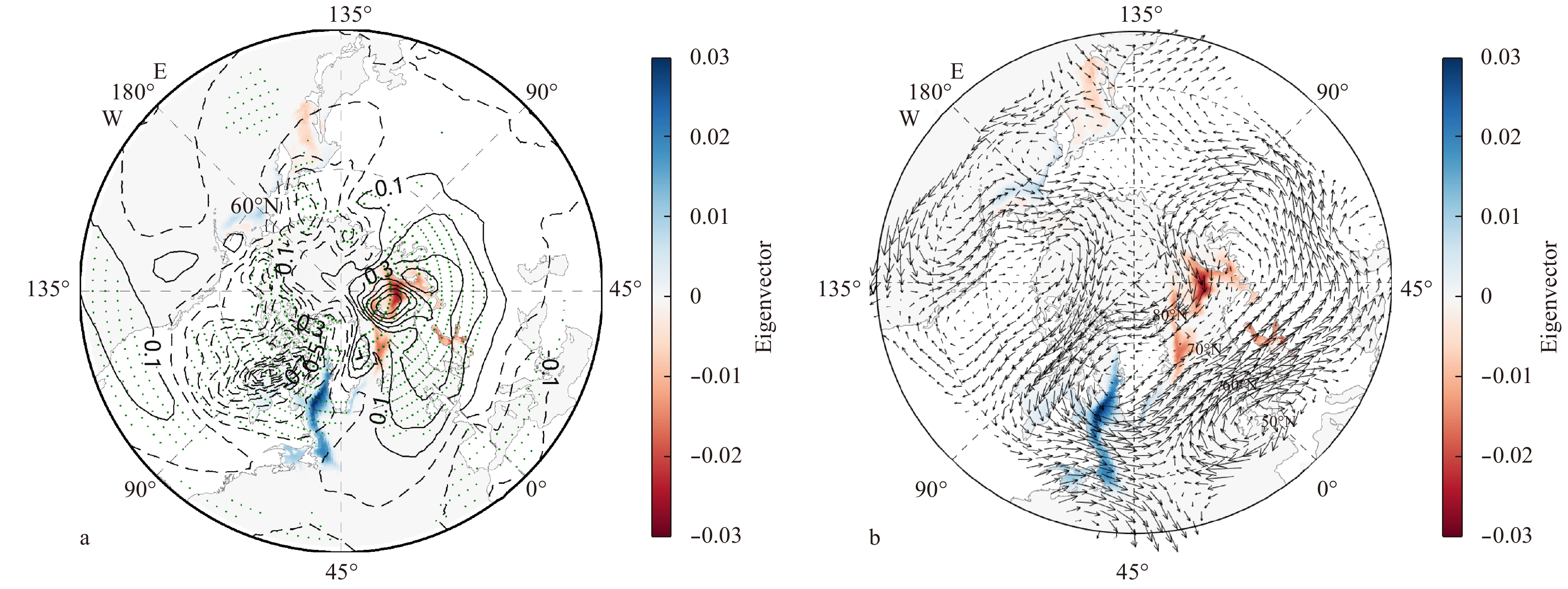
Figure 3. EOF patterns of SIC (shading) and regression map for SLP anomalies (contours) upon the leading PC time series (left) and second PC time series (right) of the SIC in winter. The patterns were constructed by linearly regressing the SLP anomalies upon the first two PC time series (lines in Fig. 1b). The regressed SLP fields have units of mb per standard deviation of PC index. The long dashed lines represent zero and negative values and solid lines represent positive values. Green dots indicate areas with a linear regression that is significant at the 90% confidence level.
Figure A3. EOF patterns of SIC (shading) and regression map for SAT anomalies (contours) (a), and heat flux anomaly (vectors) (b) upon the leading PC time series of the SIC in winter. The patterns were constructed by linearly regressing the SAT anomalies upon the leading PC time series (red bold line in Fig. A1b). The regressed fields have units of K/(W·m2) per standard deviation of PC index. The long dashed lines represent zero and negative values and solid lines represent positive values. Green dots indicate areas with a linear regression that is significant at the 90% confidence level.
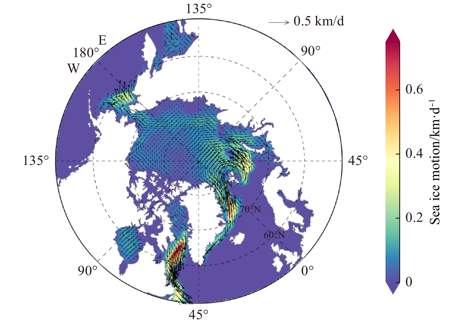
Figure A4. Concurrent winter SIM anomaly pattern associated with the leading ice EOF. Note that the shading indicates the SIM speed. The regressed SIM fields have unit of km/d per standard deviation of PC index.
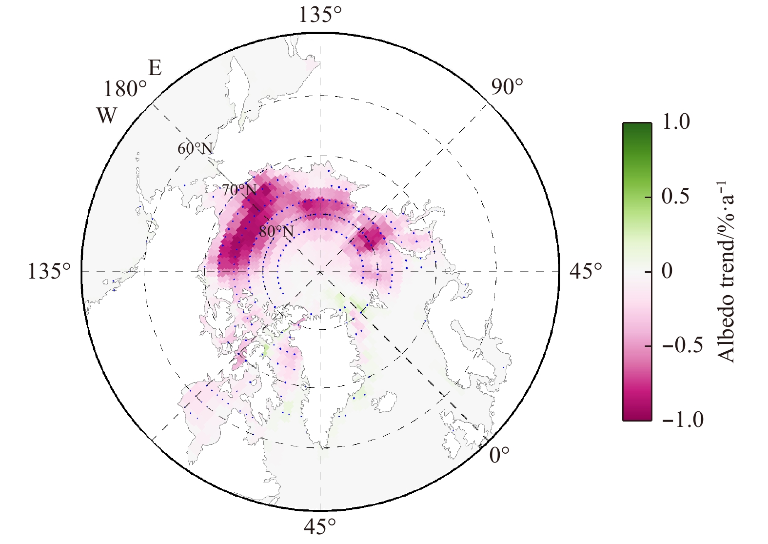
Figure 4. Surface albedo trend in the Arctic Ocean in summer (1979–2017).
Figure 5. EOF patterns of SIC (shading) and regression map for SAT anomalies (contours) upon the leading PC time series (a) and second PC time series (b) of the SIC in summer. The patterns were constructed by linearly regressing the SAT anomalies upon the first two PC time series (lines in Fig. 1b). The regressed SAT fields have units of K per standard deviation of PC index. The long dashed lines represent zero and negative values and solid lines represent positive values. Green dots indicate areas with a linear regression that is significant at the 90% confidence level.
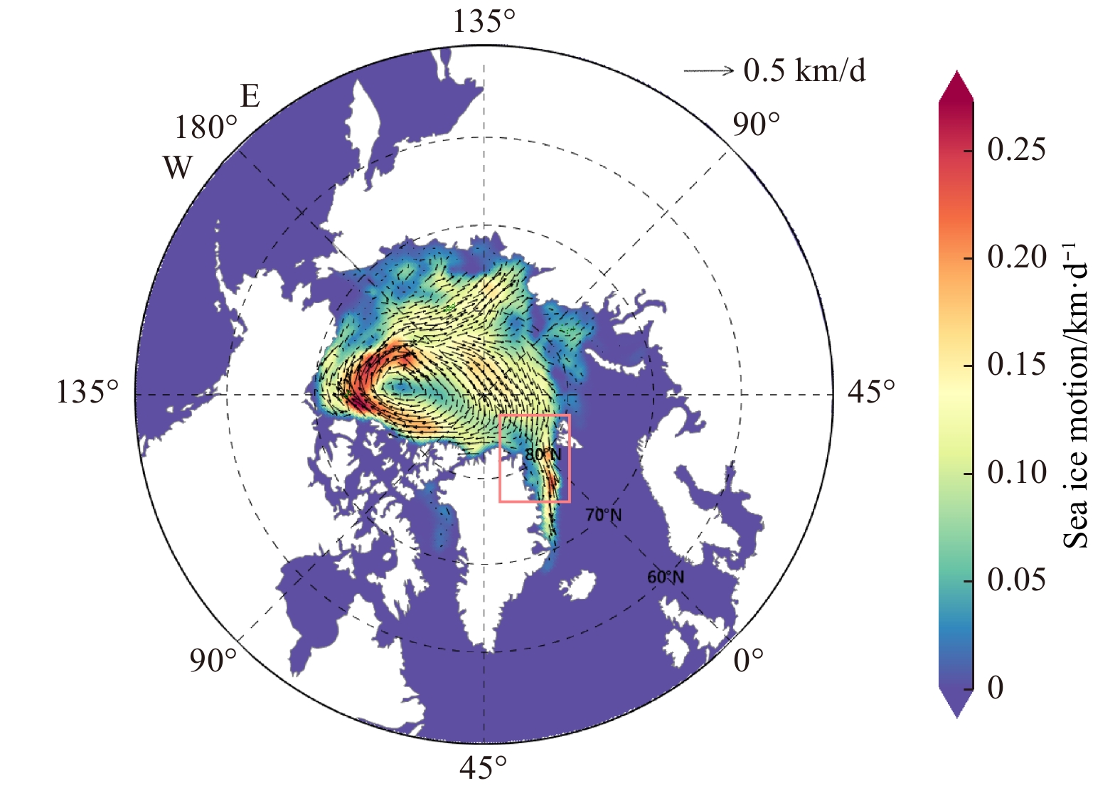
Figure 6. Concurrent summer SIM anomaly pattern associated with the leading ice EOF. Note that the shading indicates the SIM speed. The regressed SIM fields have units of km/d per standard deviation of PC index. The pink box indicates sea ice flux through the Fram Strait.
Figure A5. EOF patterns of SIC (shading) and regression map for SLP anomalies (contours) upon the leading PC time series of the SIC in summer. The patterns were constructed by linearly regressing the SLP anomalies upon the leading PC time series (red bold line in Fig. A2b). The regressed SAT fields have unit of K per standard deviation of PC index. The long dashed lines represent zero and negative values and solid lines represent positive values. Green dots indicate areas with a linear regression that is significant at the 90% confidence level.
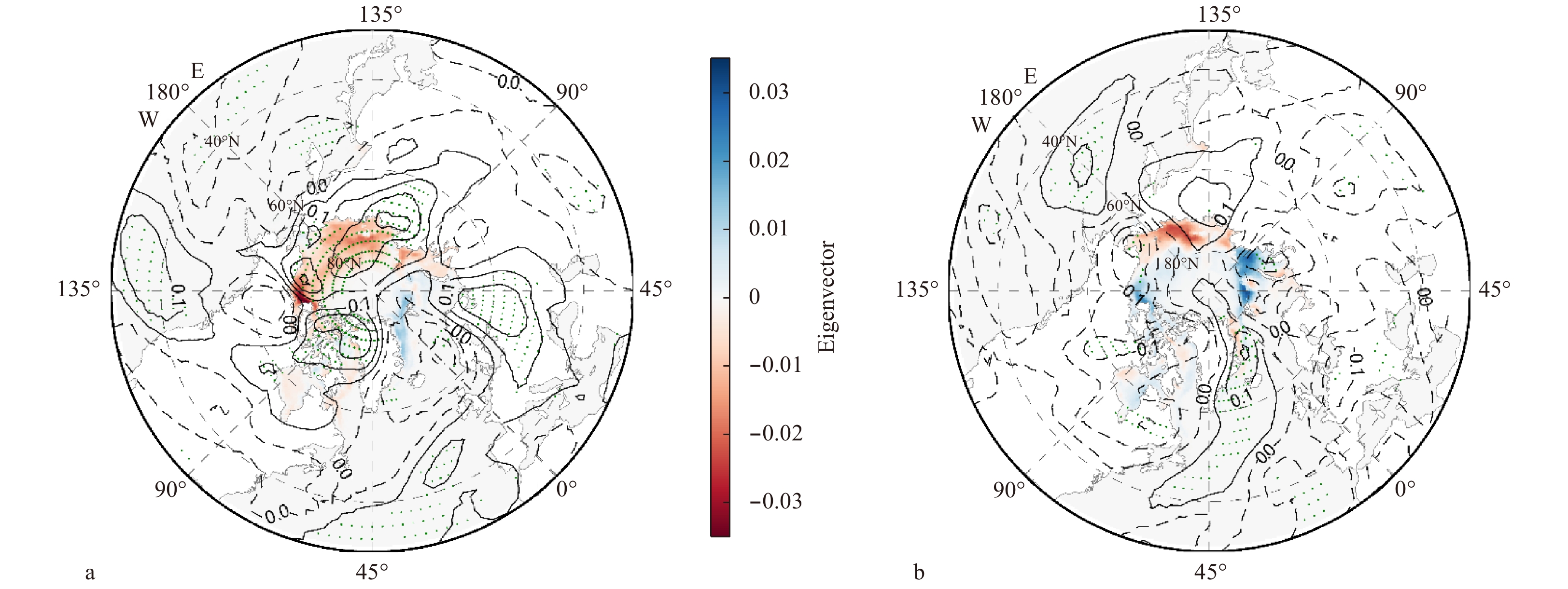
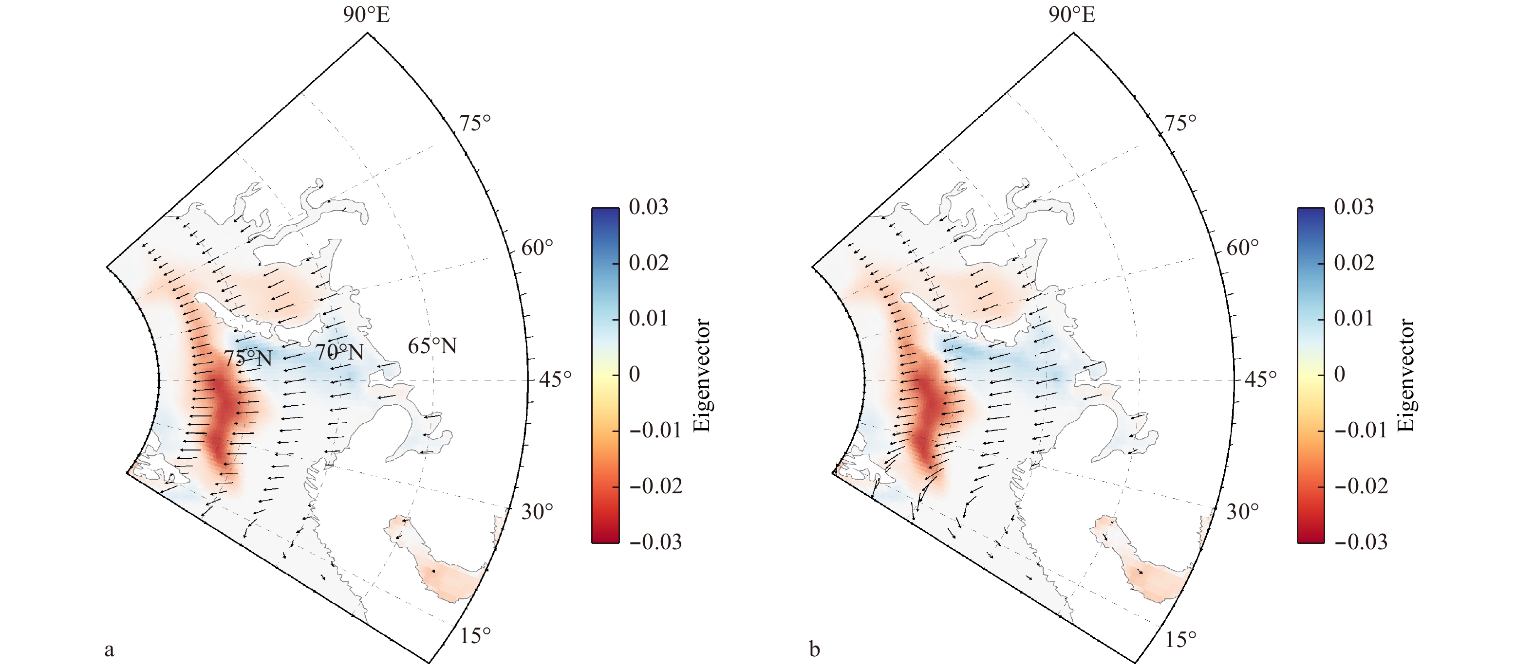
Figure A6. EOF patterns of SIC (shading) and regression map for SAT anomalies (contours) (a) and surface latent heat flux anomalies (contours) (b) upon the second pc time series of the SIC in winter. The patterns were constructed by linearly regressing the anomalies anomalies upon the socond PC time series (blue dashed line in Fig. A1b). The regressed fields have unit of K/(W·m2) per standard deviation of PC index. The long dashed lines represent zero and negative values and solid lines represent positive values. Green dots indicate areas with a linear regression that is significant at the 90% confidence level. Two green boxes are the rough boundaries of two specific analysis areas.
Figure 7. Regression map for total column water vapor and downward longwave flux (contours) and SAT (shading) anomalies upon the second EOF of the SIC in winter in the North Pacific (30°–80°N, 135°W–135°E) (a) and Hudson Bay (40°–75°N, 45°–90°W) (b). The patterns were constructed by linearly regressing the three variables upon the second PC time series (blue dashed line in Fig. 1a). The regressed SAT, total column water vapor and downward longwave flux fields have units of K, kg/m2 and W/m2 per standard deviation of PC index, respectively. Grey lines indicates downward longwave flux and colored lines indicates total column water vapor fields. The long dashed lines represent zero and negative values and solid lines represent positive values. Note that most areas are significant at the 90% confidence level.
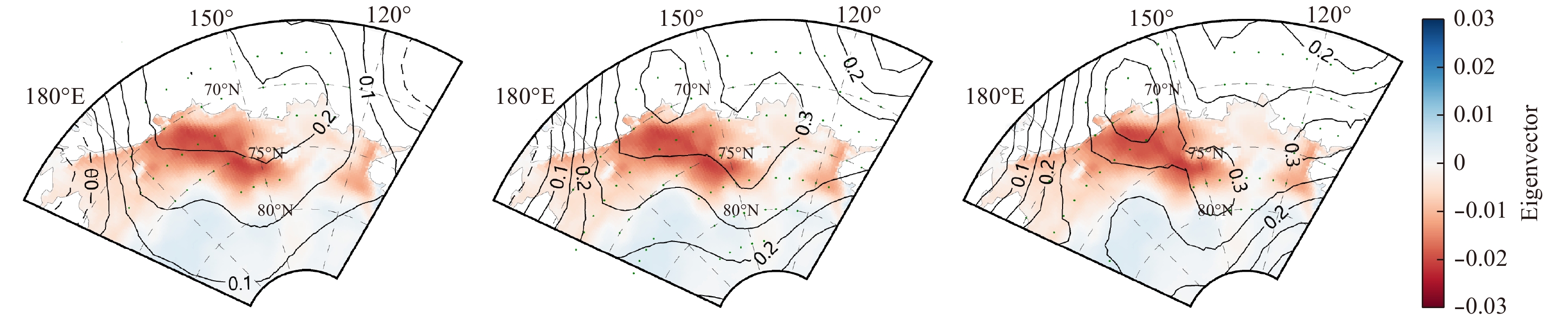
Figure 8. Concurrent winter SIM anomaly pattern associated with the second SIC EOF around the Bering Strait (40°–80°N, 135°W–135°E). Note that the shading indicates the SIM speed. The regressed SIM fields have units of km/d per standard deviation of PC index.
Figure 9. The second EOF of SIC (shading) and regression map for heat flux (a) and water vapor flux anomalies (vectors) (b) upon the second EOF of the SIC in winter in the Barents Sea (60°–80°N, 10°–90°E). The patterns were constructed by linearly regressing the two variables upon the second PC time series (blue dashed line in Fig. 1a). The regressed heat flux and water vapor flux fields have units of W/m and kg/(m·s) per standard deviation of PC index, respectively. Note that most areas are significant at the 90% confidence level.
Figure 10. Regression map for total cloud cover (contours) and surface net downward shortwave flux (shading) anomalies upon the second EOF of the SIC in summer in the marginal seas of Arctic (65°–90°N). The patterns were constructed by linearly regressing the three variables upon the second PC time series (blue dashed line in Fig. 2a). The regressed surface net downward shortwave flux fields have unit of W/m2 per standard deviation of PC index, respectively. The long dashed lines represent zero and negative values and solid lines represent positive values. Note that the green circles and purple dots indicate areas with a linear regression that is significant at the 90% confidence level for regressed cloud and downward shortwave flux fields, respectively.
Figure 11. EOF patterns of SIC (shading) and regression map for SAT anomalies (contours) upon the second PC time of the SIC in Chukchi Sea, East Siberian Sea and Laptev Sea (65°–85°N, 105°E–20°W) during summer when SAT lags the ice by 2 months (a), 3 months (b) and 4 months (c). The patterns were constructed by linearly regressing the SAT anomalies upon the second PC time series (blue dashed line in Fig. 2b). The regressed SAT fields have unit of K per standard deviation of PC index. The long dashed lines represent zero and negative values and solid lines represent positive values. Green dots indicate areas with a linear regression that is significant at the 90% confidence level.
Figure 12. Average melt onset, freeze onset, and average melt duration in days for the in the Chukchi Sea, East Siberian Sea and Laptev Sea (65°–85°N, 105°–20°W). Space between the curves indicates the melt season length and red dashed line represents its trend.


 DownLoad:
 DownLoad:


 DownLoad: