Lu Liu, Mingzhu Fu, Kaiming Sun, Qinzeng Xu, Zongjun Xu, Xuelei Zhang, Zongling Wang. The distribution of phytoplankton size and major influencing factors in the surface waters near the northern end of the Antarctic Peninsula[J]. Acta Oceanologica Sinica, 2021, 40(6): 92-99. doi: 10.1007/s13131-020-1611-3
Citation:
Lu Liu, Mingzhu Fu, Kaiming Sun, Qinzeng Xu, Zongjun Xu, Xuelei Zhang, Zongling Wang. The distribution of phytoplankton size and major influencing factors in the surface waters near the northern end of the Antarctic Peninsula[J]. Acta Oceanologica Sinica, 2021, 40(6): 92-99. doi: 10.1007/s13131-020-1611-3
Lu Liu, Mingzhu Fu, Kaiming Sun, Qinzeng Xu, Zongjun Xu, Xuelei Zhang, Zongling Wang. The distribution of phytoplankton size and major influencing factors in the surface waters near the northern end of the Antarctic Peninsula[J]. Acta Oceanologica Sinica, 2021, 40(6): 92-99. doi: 10.1007/s13131-020-1611-3
Citation:
Lu Liu, Mingzhu Fu, Kaiming Sun, Qinzeng Xu, Zongjun Xu, Xuelei Zhang, Zongling Wang. The distribution of phytoplankton size and major influencing factors in the surface waters near the northern end of the Antarctic Peninsula[J]. Acta Oceanologica Sinica, 2021, 40(6): 92-99. doi: 10.1007/s13131-020-1611-3
College of Environmental Science and Engineering, Ocean University of China, Qingdao 266100, China
2.
Key Laboratory of Marine Eco-environmental Science and Technology of Ministry of Natural Resources, First Institute of Oceanography, Qingdao 266061, China
3.
Pilot National Laboratory for Marine Science and Technology (Qingdao), Qingdao 266237, China
Funds:
The Foundation of China Ocean Mineral Resources R&D Association under contract No. DY135-E2-4; the Basic Scientific Fund for National Public Research Institutes of China under contract Nos 2018Q09 and 2018S02; the National Natural Science Foundation of China under contract Nos 41706190 and 41876231.
The waters near the Antarctic Peninsula have always been a study hot spot because of their variable and unique oceanographic conditions. To determine the distribution and possible influencing factors on phytoplankton size and abundance near the Antarctic Peninsula, a large-scale survey was conducted during the austral summer of 2018. Samples were collected in 27 stations located in the Drake Passage (DP), South Shetland Islands (SSI), and South Orkney Islands (SOI). Phytoplankton communities were described using chlorophyll a (Chl a), flow cytometry and light microscopy to cover a size range from pico- to microphytoplankton. Nanophytoplankton, especially small nanophytoplankton (2−6 μm) with abundance ranging from 0.66 ×10³ cells/mL to 8.46 ×10³ cells/mL, was predominant throughout the study area. Among different regions, there was an obvious size shift. The proportion of picophytoplankton near the Elephant Island (EI) and DP was higher than other regions, and larger cells were found mainly in east of SOI. The distribution of phytoplankton abundance detected by flow cytometry was not completely consistent with Chl a concentrations due to the contribution of larger cells to Chl a. Possible influencing factors on the phytoplankton size distribution were discussed. The properties of water masses such as temperature and salinity can influence the phytoplankton size distribution. Correlation analysis revealed that only picophytoplankton is significantly correlated with salinity. Light and Fe availability might affect phytoplankton abundance and size distribution especially near the waters of SSI and EI in this study. It was also speculated that the abundance of cryptophytes is possibly related to ice melting.
The waters near the Antarctic Peninsula have always been a focus of research because of their variable hydrologic and nutritional conditions, and they are sensitive to climate change. Phytoplankton distribution is patchy and could respond sensitively to environmental changes like fronts, marginal ice-melting zones or water masses (Schloss and Estrada, 1994; Vernet et al., 2008). Nanoplankton-sized communities were found in coastal and frontal regions including diatoms, flagellates and protozoa (Hewes et al., 1985; Becquevort, 1997; Ishikawa et al., 2002). Episodic blooms of both nano- and micro-phytoplankton commonly occur along the edge of the receding marginal ice, polynyas, and oceanic fronts (Garibotti et al., 2005; Smith et al., 2008; Vernet et al., 2008). There are also many uncertain factors affecting the abundance and size distribution of phytoplankton, so the environmental adaptability of phytoplankton remains to be discussed.
Cell size is a master functional trait and phytoplankton size structure controls the trophic organization of planktonic communities (Marañón, 2015). Therefore, analyses of phytoplankton size structure are necessary to better understand controls on phytoplankton dynamics. The size range of phytoplankton communities in Antarctic waters has been previously described. Numerous studies have shown that Antarctic phytoplankton communities are often dominated by organisms <20 μm in size (Ishikawa et al., 2002). According to García-Muñoz’s research (García-Muñoz et al., 2013), total chlorophyll a (Chl a) near the South Shetland Islands (SSI) was largely due to nanophytoplanktonic cells (<20 μm), except for the station closest to the Antarctic Peninsula (AP), where microplanktonic cells (>20 μm) predominated (Rodríguez et al., 2002). Although these studies have provided useful information on the distribution patterns of phytoplankton size in the Southern Ocean, they did not capture the more precise size ranges and large-scale shifts in phytoplankton size.
The size structure of phytoplankton is usually analyzed through fractionation of chlorophyll. The information obtained through this method is nonconclusive due to filtering error. With the advent of flow cytometry (FCM), the predominant size of phytoplankton in the Antarctic has been described. FCM has the advantage of counting tens to hundreds of cells per second as well as distinguishing phytoplankton cells and non-living particles (Green et al., 2003). This technology is widely used to record nanophytoplankton (2−20 μm) and picophytoplankton (<2 μm) including Prochlorococcus, Synechococcus and pico-eukaryotes (Rodríguez et al., 2002; García-Muñoz et al., 2013). FCM analysis has proven to be highly efficient in pico- and nanophytoplankton analysis because of its facility and precision (Blanchot and Rodier, 1996; Zhang et al., 2012). However, FCM does not resolve scarcer and larger phytoplankton, particularly microplankton (>20 μm equivalent spherical diameter (ESD)) (Sosik et al., 2010). Thus, it is vital to employ a combination of FCM and light microscopy to describe the entire size spectrum of phytoplankton.
This study seeks to analyze the size structure and composition of Antarctic phytoplankton using a combination of flow cytometry and light microscopy. These methods permit characterizing of the complete size and abundance distribution of phytoplankton. This study has also observed shifts in phytoplankton size classes and abundance in water columns with diverse oceanographic and hydrographical features at the large regional scale.
2.
Materials and methods
2.1
Samples collection
This study collected water samples from 27 stations near the AP in January and February 2018 (Fig. 1). Two stations, SR14 and SR17, were situated in the Drake Passage (DP), three stations, including RY0A, RY0B, and DZ07 were near the SSI, and the other stations were located near the South Orkney Islands (SOI). Elephant Island (EI) is located between SOI and SSI. At each station, water samples were collected at the surface (depth, 0−5 m) using bottles attached to conductivity temperature depth (CTD)-profiling units. Two liters of seawater was filtered through Whatman GF/F glass fiber filters, and the filters were stored at −150°C until Chl a measurement. In addition, 1.5 L seawater samples were collected and fixed with Lugol’s solution in situ for microscopy analysis. Approximately 5 mL of the surface seawater samples collected for FCM analysis was pre-filtered through a 20-μm mesh to remove impurities such as larger particles and then fixed with a mix of 10% parafomaldehyde and 0.5% glutaraldehyde.
Figure
1.
Study area and sampling stations in the Southern Ocean. The filled blue dots show the locations of the 27 stations. SOI, South Orkney Islands; EI, Elephant Island; DP, Drake Passage; SSI, South Shetland Islands. The solid yellow curve indicates the transect from SSI to SOI.
Two thousands (V2) milliliter of seawater was filtered on GF/F filters. The filters were transported to the laboratory, and photosynthetic pigments were extracted by immersing the filters in 10 mL (V1) of 90% acetone. After 24 h in the dark, the fluorescence (Rb) in the supernatants was determined by measuring using Turner TD-700. Two drops of HCl were then added, and the extracts re-read (Ra) after acidification (Holm-Hansen et al., 1965). The concentration (c) of Chl a was calculated by the formula c=Fd·(Rb–Ra)·V1/V2. Fd is the constant of the instrument, and the value is 2.046.
2.3
Flow cytometry analysis
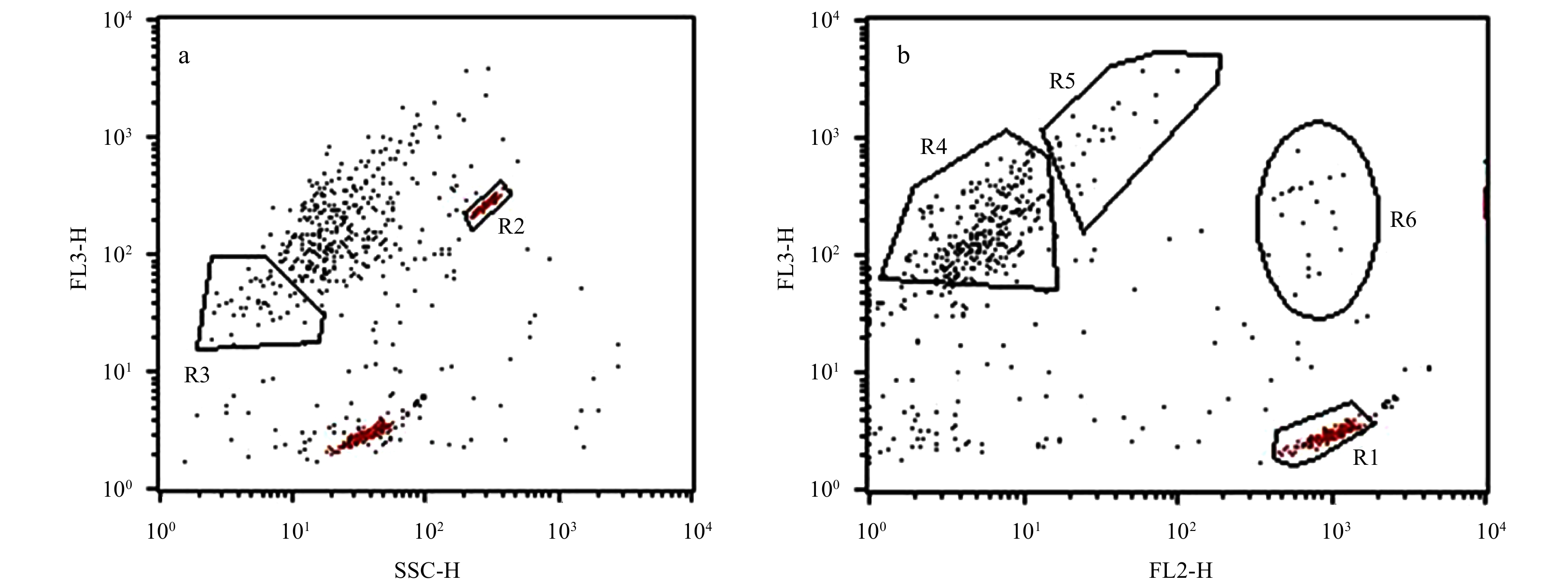
The samples were transported to the laboratory and analyzed using a flow cytometer (FACScalibur, Becton-Dickinson Company). The following acquisition parameter settings were defined: forward light scatter (FSC) = E00; side light scatter (SSC) = 274 V; FL1 = 650 V; FL2=520 V; FL3=458 V. FSC and SSC were used to estimate cells content and size. FL3 was used to detect red fluorescence, and FL2 was used to detect orange fluorescence. The flow rate was 60 μL/min, and the measuring time was 90 s, which was calibrated at the beginning and at the end of the experiment. Fluorescence and SSC were monitored using 2 μm and 6.19 μm diameter yellow/green fluorescent beads. Data were acquired and analyzed with the CellQuest software. Four size groups of eukaryotic cells were discriminated on bivariate plots of SSC versus FL3 and FL2 versus FL3 (Fig. 2). R1 and R2 were respectively 2 μm and 6.19 μm fluorescent beads that were used as controls. Three groups, R3, R4, and R5, represented picophytoplankton (<2 μm ESD), small nanophytoplankton (about 2−6 μm), and medium nanophytoplankton (slightly >6 μm). They were discriminated by cell size and fluorescence intensity. Cells with similar size and fluorescence intensity were clustered into one group, which can separate from other groups. Group R6 consisted of the flagellate cryptophytes, and easily separated from the common size compartment owing to the orange fluorescence of phycoerythrin. However, not all samples could be clearly discriminated into four groups. Phytoplankton abundance in Stations SR17, DC01, D305, and DC11 was only counted with total abundance.
Figure
2.
Flow cytometric plots of SSC vs. FL3 (a), and FL2 vs. FL3 (b). R1, 2 μm beads; R2, 6.19 μm beads; R3, picophytoplankton, <2 μm; R4, small nanophytoplankton, about 2−6 μm; R5, medium nanophytoplankton, >6 μm slightly; R6, cryptophytes.
Microscopy analysis was conducted to measure phytoplankton size and identify cells >10 μm in length to supplement the results of FCM. This study selected nine stations at intervals to represent different regions for microscopy analysis. Additional stations with high values of Chl a concentrations and an abundance of the four groups (R3-6) were also included. The 1.5 L samples in plastic bottles were sedimented for 48 h, and the supernatant was aspirated off to give a final concentrated volume of 20 mL. Concentrated samples of about 0.5 mL were identified and counted at 200× to 400× magnification using a Nikon Eclipse Ti2-U inverted microscope. Phytoplankton length was measured using NIS-Elements D 4.51.00 software connected with microscopy.
2.5
Data processing
The data were visualized in Ocean Data View. Statistical analysis was performed using a Canoco 4.5 program package. This study conducted detrended correspondence analysis (DCA) of the biological data to decide between unimodal or linear methods. Analysis results were stored in Log View. If the longest gradient is larger than 4.0, unimodal methods are selected (Canonical correspondence analysis), whereas if the longest gradient is shorter than 3.0, the linear method is probably a better choice (Redundancy analysis, RDA). Monte Carlo permutation tests were performed to test the significance of the environmental factors. In this test, an estimate of the distribution of the test data under the null hypothesis is obtained in the following way. The null hypothesis states that the response (the species composition) is independent of the environmental variables. If this hypothesis is true, then it does not matter which observation of explanatory variable values is assigned to which observation of species composition (Lepš and Šmilauer, 2003).
3.
Results
3.1
Oceanographic parameters
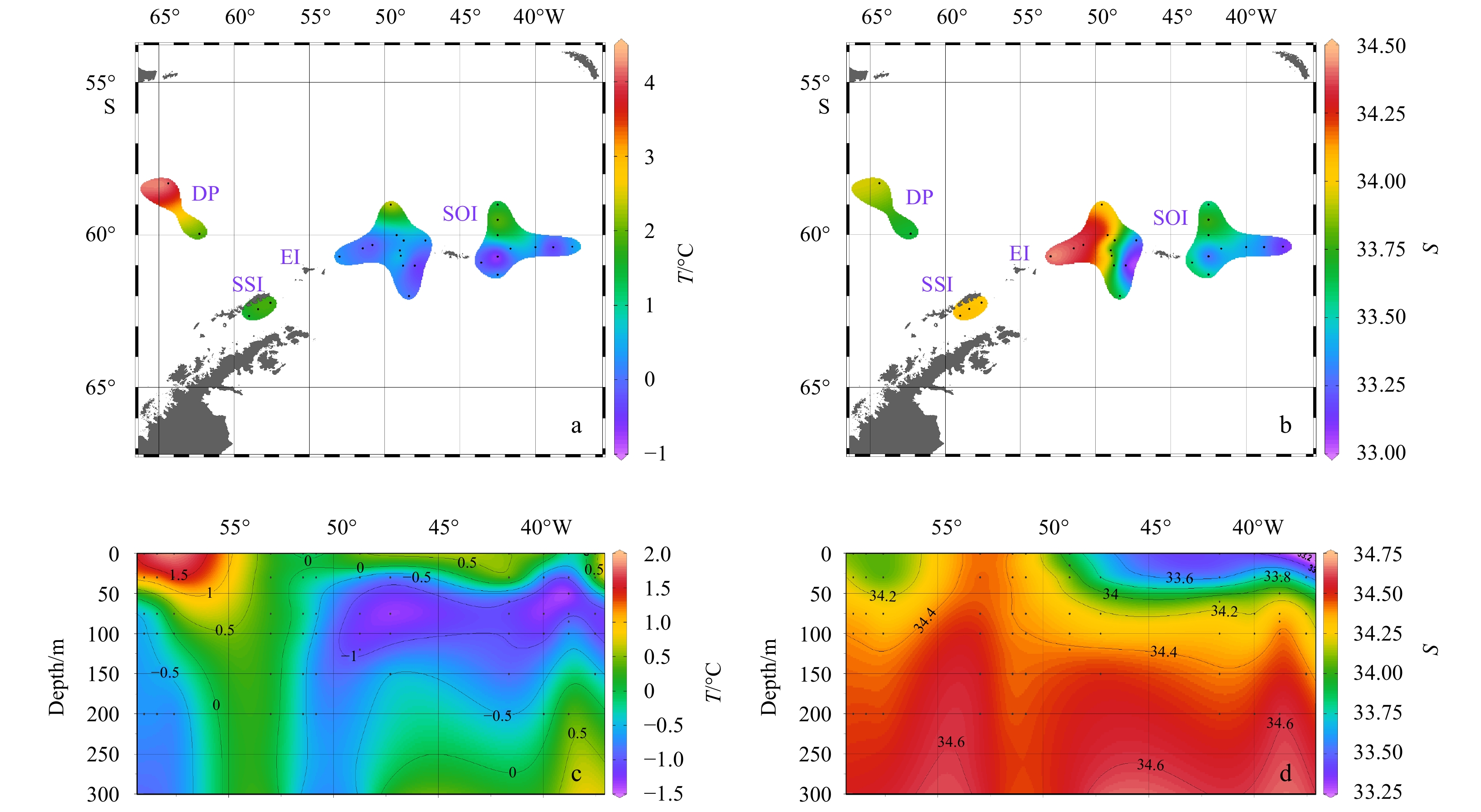
The oceanographic parameters at the sampling sites, included temperature (Figs 3a, c) and salinity (Figs 3b, d). The temperature of the surface waters (Fig. 3a) was generally low, about 0°C. The temperature in the north was slightly higher than in the south. The highest temperature (4.17°C) was in DP, which was the northernmost station in the study area. The salinity (Fig. 3b) of the survey area was higher in the west than in the east and higher near EI. A profile of temperature (Fig. 3c) and salinity (Fig. 3d) along the SSI-SOI transect showed that stations near the SSI were deeply mixed while other stations around SOI were shallow.
Figure
3.
Surface and transect (SSI-SOI) distribution of temperature and salinity. a. Surface temperature; b. surface salinity; c. transect temperature; d. transect salinity.
3.2
Distribution of Chl a and total abundance of phytoplankton by FCM
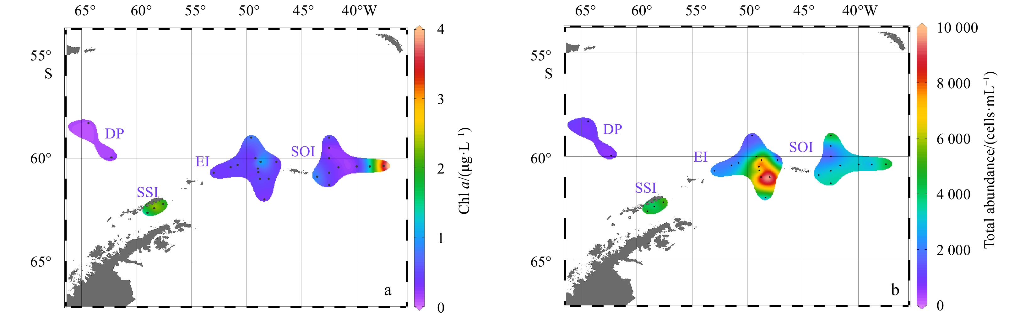
Chl a concentrations in Fig. 4a ranged from 0.10 μg/L to 3.56 μg/L at the surface. Chl a concentrations fluctuated in the study area. The lowest concentration of Chl a was observed in Station SR14 at DP, whereas the highest concentration was at Station DC11, east of the other stations. Chl a concentrations were also higher in the three stations near the SSI than in the other stations around SOI.
Figure
4.
Distribution of Chl a concentration (μg/L) (a) and total abundance (cells/mL) (b) based on FCM.
Flow cytometry analysis indicated that there were no relevant signals indicating the presence of Prochlorococcus and Synechococcus. The total abundance of eukaryotic cells (Fig. 4b) ranged from 6.08 cells/mL in Station SR17 to 9.71×10³ cells/mL in Station M2. The highest abundance was observed in southwest of SOI, while the lowest was in DP. The abundance was also relatively high near the SSI.
3.3
Distribution of phytoplankton size and abundance by FCM
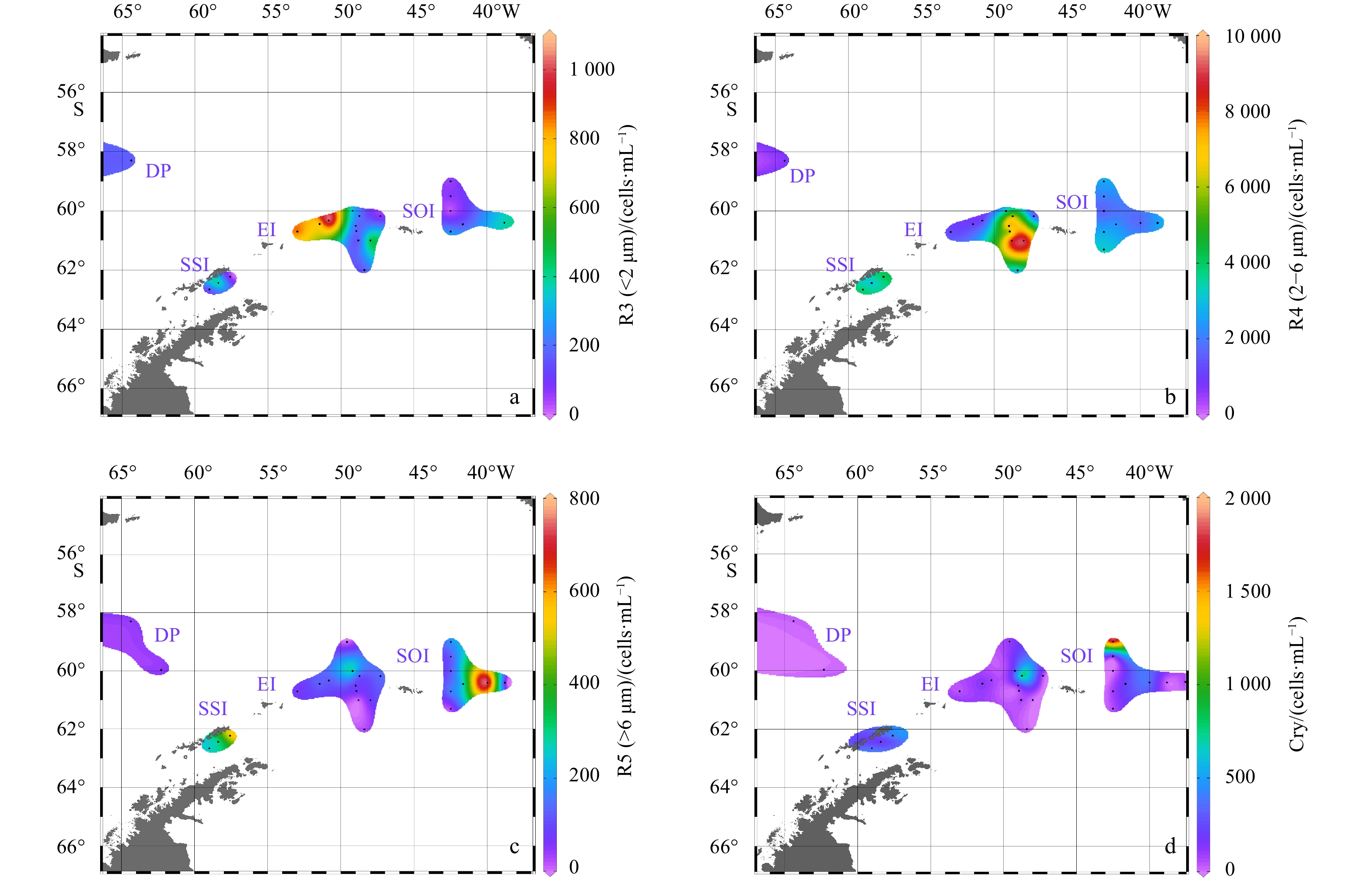
This study discriminated four groups of eukaryotic cells that roughly correspond to picophytoplankton (R3), “small nano” (R4), “medium nano” (R5), and cryptophytes (Cry). The distribution characteristics of their abundance are shown in Fig. 5. Phytoplankton in Stations DC01, DC11, D305 and SR17 could not clearly distinguish by FCM, hence, there were no data from these stations. Picophytoplankton abundance ranged from 21.72 cells/mL at Station D507 to 1.05×10³ cells/mL at Station DA06. High phytoplankton abundance was observed northeast of EI. “Small nano” was the predominant group in the study area with high abundance ranging from 0.66 ×10³ cells/mL to 8.46 × 10³ cells/mL. The highest abundance occurred in southwest of SOI, whereas low abundance was observed in DP. Two areas with relatively high abundance of “medium nano” occurred in east of SOI and in the vicinity of SSI. The area with the lowest abundance of “medium nano” was in the DP. The last group, Cry had high abundance in the north with the highest value (8.14×10² cells/mL) at Station DA09. Cry abundance around SSI and stations near the northwest of SOI was also relatively high. The abundance of cryptophytes at other stations was similar to one another.
Figure
5.
Distribution of eukaryotic cell abundance in four groups. a. R3, picophytoplankton; b. R4, “small nano”; c. R5, “medium nano”; d. Cry, cryptophytes.
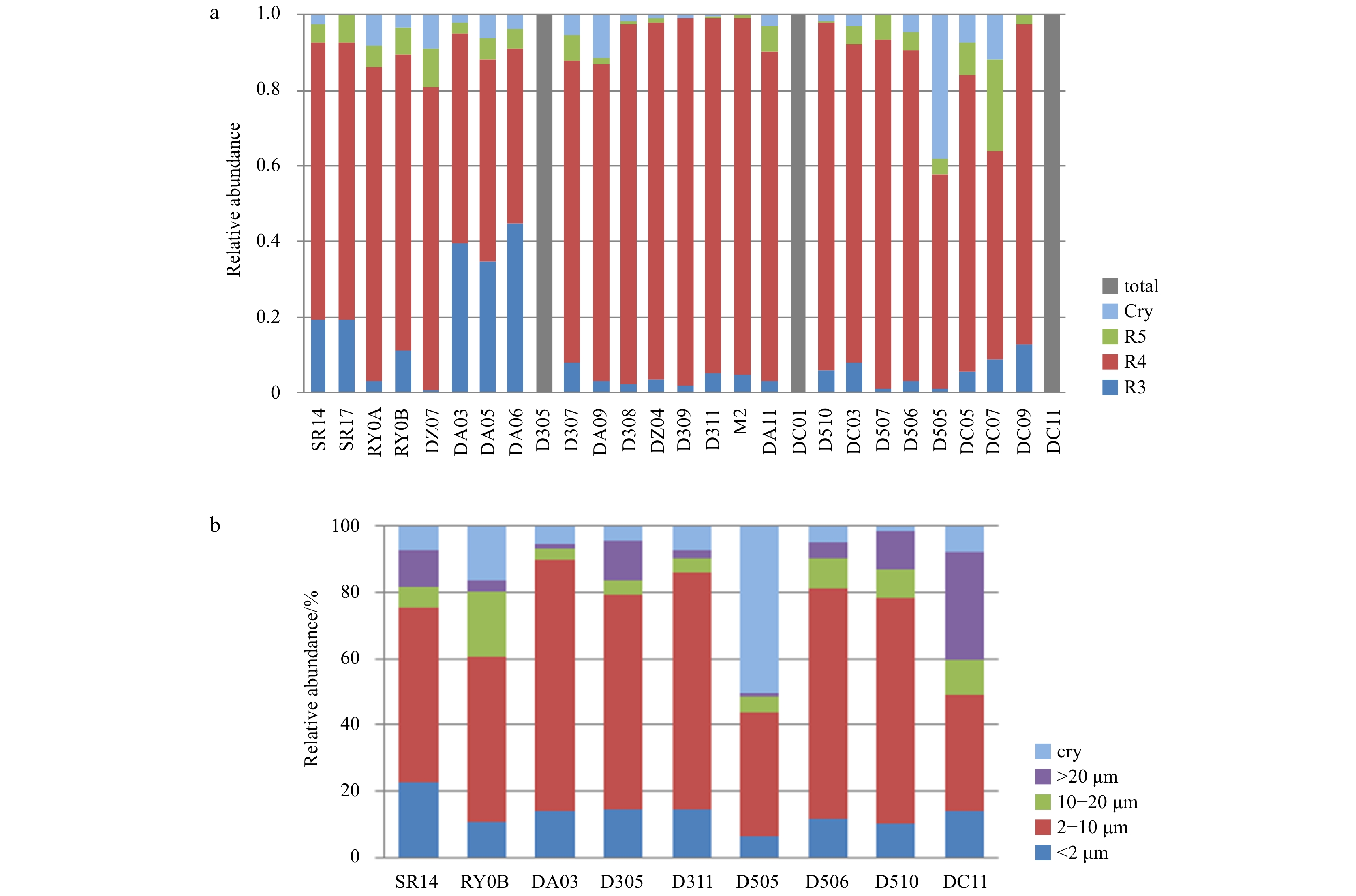
The size composition of phytoplankton communities obtained by FCM and microscopy is presented in Fig. 6. The predominant group was R4 (2–6 μm). The results of microscopy identification were consistent to a large degree with the trend obtained by FCM. Five size groups are presented. Phytoplankton with cell lengths between 2 μm and 10 μm were predominant at most stations. Picophytoplankton <2 μm in length occupied a lower proportion of the phytoplankton at these stations. Cryptophytes were predominant at Station D505, which is the same result obtained with FCM. The relative abundance of microphytoplankton >20 μm in length significantly increased at Station DC11.
Figure
6.
Size composition of phytoplankton communities based on FCM (a) and microscopy (b).
3.5
Correlation between biological and environmental parameters
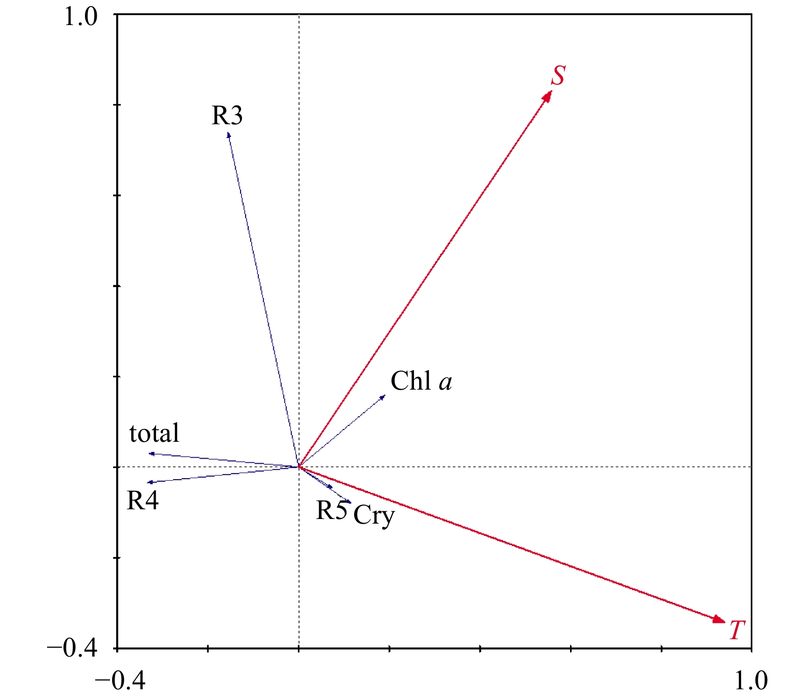
Multivariate ordination techniques were employed to explore the relationships between phytoplankton abundance in different size categories and environmental parameters. DCA showed the maximum gradient length was less than 3; therefore, a linear model was applied. An RDA ordination diagram was shown in Fig. 7. Salinity was positively correlated with R3 (indicated by angles <90° between arrows of groups and environmental variables) and slightly negatively correlated with other groups. Temperature was positively correlated with Groups R5 and Cry, and negatively correlated with other groups. Monte Carlo permutation tests were carried out between different groups and environmental factors. The permutation numbers were 499. The results indicate that R3 (picophytoplankton) was significantly positively correlated (P=0.004) with salinity. The other groups and total Chl a had no significant correlation with environmental factors.
Figure
7.
Phytoplankton groups and environmental factors biplot based on RDA.
4.1
Distribution patterns of the different phytoplankton size groups
In this study, the distributions of phytoplankton size and abundance were studied on a larger scale than most prior studies by a variety of analysis methods. In general, nanophytoplankton, especially small nano-, was predominant in the study area. Previous studies agree with this conclusion. The results of Egas et al. (2017) indicated a strong predominance of nanophytoplankton in western Antarctic Peninsula, and nanodiatoms, particularly Fragilariopsis spp., numerically predominated the diatom community in the Southern Ocean (Ishikawa et al., 2002). The investigation of SSI showed that nanophytoplanktonic cells (<20 μm) comprised 84% of the total chlorophyll a (García-Muñoz et al., 2014). Among different regions, there was an obvious size proportion shift. The proportion of picophytoplankton near the EI and DP was higher than in other regions. Larger cells were found mainly in the east of SOI. Most of the previous studies focused on a localized region for size division, and it is rare to study size distribution on such a large scale.
Phytoplankton abundance measured by FCM increased from DP and SSI to the west of SOI, and then decreased to east of SOI. This trend does not exactly in line with Chl a concentrations. Phytoplankton abundance measured by FCM generally consisted of cells less than 10 μm. However, according to microscope observations, there were several stations, such as DC11 and DC07, with a relatively high proportion of microphytoplankton comprised mainly of small diatoms. Studies measuring the amount of Chl a collected by filters of different pore size suggest that, as total phytoplankton biomass increases, the biomass in each size class keeps growing until it reaches an upper limit. This upper limit is higher for progressively larger cell sizes (Marañón et al., 2012; Ward et al., 2014). This implies that, beyond a certain limit, more phytoplankton biomass can be added only if larger size classes are added (Marañón, 2015). This study speculated that increased Chl a concentrations were largely contributed by the larger-size phytoplankton. As a result, the total abundance by FCM was not in line with Chl a. Therefore, it is not adequate to describe and study phytoplankton biomass using only Chl a. Other methods are needed to study the composition of different cell sizes.
4.2
Possible influencing factors on the phytoplankton size distribution
Temperature and salinity were analyzed to explore potential causes of the observed distribution of phytoplankton size in this study. Morán et al. (2010) found that temperature alone explained most of the variability in the relative contribution of picophytoplankton to total biomass. Because the time span of this study was only one month, there was little variation in temperature. No correlation was observed between phytoplankton abundance and temperature. Correlation analysis revealed that only picophytoplankton are significantly correlated with salinity. Salinity in Antarctic waters during the austral summer is generally low due to melting ice and runoff. The water column near the SSI is from the Weddell Sea with iron-rich, saline, and deeply mixed shelf waters (Hewes, 2009). Therefore, this water mass is characteristic of higher salinity. Using size classed Chl a data collected at SSI in 1999–2007 during the summer, Chl a concentrations in different size groups were tested for having a bell-shaped (unimodal) pattern in relaiton to the salinity gradient. Maximal values occurred at salinities of 34.0–34.2. Pico- and nanoplankton Chl a decreased significantly from mid (34) to low salinity waters. Microplankton tended to decrease at lower salinities, but the decrease was not significant (Hewes, 2009). Picoeukaryotes were sensitive to environmental changes (Zhang et al., 2012), and smaller cells increased at a rate faster than the microplankton (Hewes, 2009). Therefore, smaller cells could quickly respond to environmental conditions and reach high abundance. To sum up, the positive correlation between picophytoplankton abundance and salinity observed in the present study when S<34 might reflect the quick response of smaller cells to environmental changes.
Light availability appears to be an important factor for phytoplankton size structure in the Antarctic. Although phytoplankton have developed an adaptive strategy to utilize low irradiance (Agawin et al., 2002), they may be light-limited in Antarctic waters, particularly in turbid coastal waters and deeply mixed oceanic waters (Sakshaug and Holm-Hansen, 1986). The results indicated that waters near the SSI and EI were deeply mixed, which means the growth of phytoplankton might be light limited to some degree. Small cells are less heavily affected by the package effect and cope better with reduced light conditions (Cermeño et al., 2005), which explains their increased biomass contribution. Enrichment experiments have provided strong evidence for the importance of iron availability in regulating primary productivity and phytoplankton biomass in the Southern Ocean (Olson et al., 2000). Light and/or Fe availability might affect phytoplankton abundance and size distribution, especially near the waters of SSI and EI.
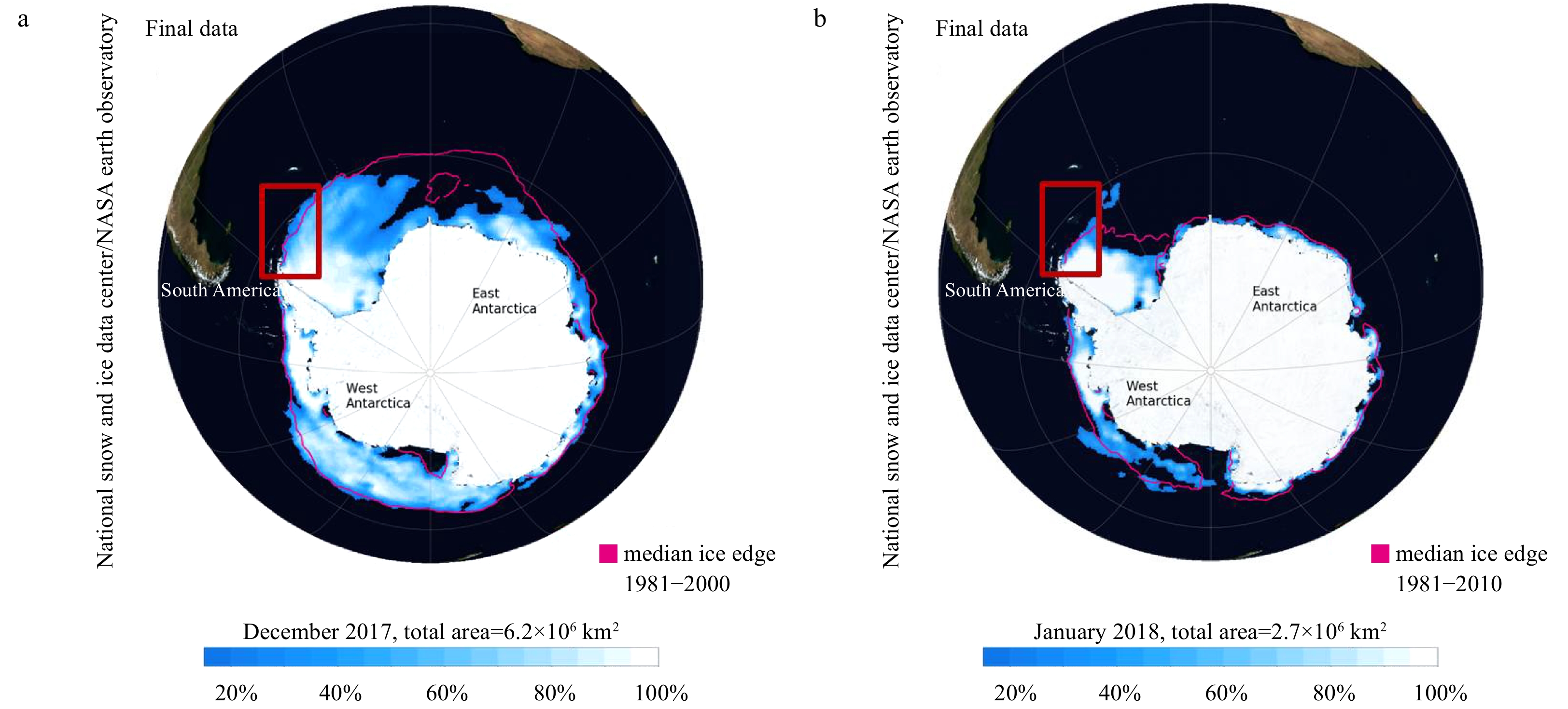
It was also important to assess the distribution of cryptophytes. FCM and microscopic analyses confirmed that cryptophytes were distributed near the SSI (Stations RY0B and DZ07) and north of SOI (Stations DA09 and D505), where the ice area was retreating. Many previous studies have shown that the melting ice is closely related to the distribution of cryptophytes (Buma et al., 1992; Garibotti et al., 2003; Korb et al., 2010). Korb et al. (2010) found that cryptophytes accounted for over half of the total phytoplankton count. Over the South Scotia Ridge, a high biomass of cryptophytes was found along the retreating ice edge (Jacques and Panouse, 1991; Buma et al., 1992). A survey conducted by Garibotti et al. (2003) revealed that cryptophyte assemblages in the seasonal ice zone of the Antarctic Peninsula are an annual occurrence. Sea ice concentration images of Antarctic are shown in Fig. 8 (Fetterer et al., 2017; ftp://sidads.colorado.edu/DATASETS/NOAA/G02135/). Stations near 60°S were located just north of the South Scotia Ridge where part of this region was covered with sea ice in December 2017. By January of 2018, the sea ice had retreated near the SOI. Although there is no accurate sea ice data for each station, it can be speculated that the abundance of cryptophytes is possibly related to ice melting.
As mentioned above, there are a variety of methods that can be used to study phytoplankton size, including fractionation of chlorophyll, FlowCAM, FCM, microcopy and so on. Each method has its own advantages and disadvantages. For examples, in previous research, it has been reported that different size groups could be obtained with FCM (Rodríguez et al., 2002; García-Muñoz et al., 2013), which not only used of fluorescence to distinguish phytoplankton but also allowed the analysis of phytoplankton size spectra. Since phytoplankton cells larger than 10 μm, ESDs were not detected by FCM, microscopy can provide supplementary information and verify the findings of this study on phytoplankton size distribution. Therefore, it is necessary to adopt a variety of methods for analysis.
In this study, Chl a, FCM, and light microscopy were used to cover sizes ranging from pico- to microphytoplankton. Although the results obtained by different methods cannot be compared directly, they can support each other and provide more comprehensive and conclusive information on the size composition and distribution of phytoplankton.
Acknowledgements
This work was supported by the 34th Chinese National Antarctic Research Exploration with R/V Xiangyanghong 01 scientific expedition vessel (JDKC0518013).
Agawin N S R, Agustí S, Duarte C M. 2002. Abundance of Antarctic picophytoplankton and their response to light and nutrient manipulation. Aquatic Microbial Ecology, 29(2): 161–172
[2]
Becquevort S. 1997. Nanoprotozooplankton in the Atlantic sector of the Southern Ocean during early spring: biomass and feeding activities. Deep-Sea Research Part II: Topical Studies in Oceanography, 44(1–2): 355–373. doi: 10.1016/S0967-0645(96)00076-8
[3]
Blanchot J, Rodier M. 1996. Picophytoplankton abundance and biomass in the western tropical Pacific Ocean during the 1992 El Niño year: results from flow cytometry. Deep-Sea Research Part I: Oceanographic Research Papers, 43(6): 877–895. doi: 10.1016/0967-0637(96)00026-X
[4]
Buma A G J, Gieskes W W C, Thomsen H A. 1992. Abundance of Cryptophyceae and chlorophyll b-containing organisms in the Weddell-Scotia Confluence area in the spring of 1988. Polar Biology, 12(1): 43–52
[5]
Cermeño P, Marañón E, Rodríguez J, et al. 2005. Size dependence of coastal phytoplankton photosynthesis under vertical mixing conditions. Journal of Plankton Research, 27(5): 473–483. doi: 10.1093/plankt/fbi021
[6]
Egas C, Henríquez-Castillo C, Delherbe N, et al. 2017. Short timescale dynamics of phytoplankton in Fildes Bay, Antarctica. Antarctic Science, 29(3): 217–228. doi: 10.1017/S0954102016000699
[7]
Fetterer F, Knowles K, Meier W N, et al. 2017 Updated Daily. Sea Ice Index, Version 3. [Antarctic, Sea Ice Concentration]. Boulder, Colorado USA: National Snow and Ice Data Center
[8]
García-Muñoz C, Lubián L M, García C M, et al. 2013. A mesoscale study of phytoplankton assemblages around the South Shetland Islands (Antarctica). Polar Biology, 36(8): 1107–1123. doi: 10.1007/s00300-013-1333-5
[9]
García-Muñoz C, Sobrino C, Lubián L M, et al. 2014. Factors controlling phytoplankton physiological state around the South Shetland Islands (Antarctica). Marine Ecology Progress Series, 498: 55–71. doi: 10.3354/meps10616
[10]
Garibotti I A, Vernet M, Ferrario M E, et al. 2003. Phytoplankton spatial distribution patterns along the western Antarctic Peninsula (Southern Ocean). Marine Ecology Progress Series, 261: 21–39. doi: 10.3354/meps261021
[11]
Garibotti I A, Vernet M, Ferrario M E. 2005. Annually recurrent phytoplanktonic assemblages during summer in the seasonal ice zone west of the Antarctic Peninsula (Southern Ocean). Deep-Sea Research Part I: Oceanographic Research Papers, 52(10): 1823–1841. doi: 10.1016/j.dsr.2005.05.003
[12]
Green R E, Sosik H M, Olson R J. 2003. Contributions of phytoplankton and other particles to inherent optical properties in New England continental shelf waters. Limnology and Oceanography, 48(6): 2377–2391. doi: 10.4319/lo.2003.48.6.2377
[13]
Hewes C D. 2009. Cell size of Antarctic phytoplankton as a biogeochemical condition. Antarctic Science, 21(5): 457–470. doi: 10.1017/S0954102009990125
[14]
Hewes C D, Holm-Hansen O, Sakshaug E. 1985. Alternate carbon pathways at lower trophic levels in the Antarctic food web. In: Siegfried W R, Condy P R, Laws R M, eds. Antarctic Nutrient Cycles and Food Webs. Berlin, Heidelberg: Springer, 277–283
[15]
Holm-Hansen O, Lorenzen C J, Holmes R W, et al. 1965. Fluorometric determination of chlorophyll. ICES Journal of Marine Science, 30(1): 3–15. doi: 10.1093/icesjms/30.1.3
[16]
Ishikawa A, Wright S W, Van Den Enden R, et al. 2002. Abundance, size structure and community composition of phytoplankton in the Southern Ocean in the austral summer 1999/2000. Polar Bioscience, 15: 11–26
[17]
Jacques G, Panouse M. 1991. Biomass and composition of size fractionated phytoplankton in the Weddell-Scotia Confluence area. Polar Biology, 11(5): 315–328
[18]
Korb R E, Whitehouse M J, Gordon M, et al. 2010. Summer microplankton community structure across the Scotia Sea: implications for biological carbon export. Biogeosciences, 7(1): 343–356. doi: 10.5194/bg-7-343-2010
[19]
Lepš J, Šmilauer P. 2003. Multivariate Analysis of Ecological Data Using CANOCO. Cambridge: Cambridge University Press
[20]
Marañón E. 2015. Cell Size as a key determinant of phytoplankton metabolism and community structure. Annual Review of Marine Science, 7: 241–264. doi: 10.1146/annurev-marine-010814-015955
[21]
Marañón E, Cermeño P, Latasa M, et al. 2012. Temperature, resources, and phytoplankton size structure in the ocean. Limnology and Oceanography, 57(5): 1266–1278. doi: 10.4319/lo.2012.57.5.1266
[22]
Morán X A G, López-Urrutia Á, Calvo-Díaz A, et al. 2010. Increasing importance of small phytoplankton in a warmer ocean. Global Change Biology, 16: 1137-44.
[23]
Olson R J, Sosik H M, Chekalyuk A M, et al. 2000. Effects of iron enrichment on phytoplankton in the Southern Ocean during late summer: active fluorescence and flow cytometric analyses. Deep-Sea Research Part II: Topical Studies in Oceanography, 47(15–16): 3181–3200. doi: 10.1016/S0967-0645(00)00064-3
[24]
Rodríguez J, Jiménez-Gómez F, Blanco J M, et al. 2002. Physical gradients and spatial variability of the size structure and composition of phytoplankton in the Gerlache Strait (Antarctica). Deep-Sea Research Part II: Topical Studies in Oceanography, 49(4–5): 693–706. doi: 10.1016/S0967-0645(01)00119-9
[25]
Sakshaug E, Holm-Hansen O. 1986. Photoadaptation in Antarctic phytopfankton: variations in growth rate, chemical composition and P versus I curves. Journal of Plankton Research, 8(3): 459–473. doi: 10.1093/plankt/8.3.459
[26]
Schloss I, Estrada M. 1994. Phytoplankton composition in the Weddell-Scotia Confluence area during austral spring in relation to hydrography. Polar Biology, 14(2): 77–90
[27]
Smith R C, Martinson D G, Stammerjohn S E, et al. 2008. Bellingshausen and western Antarctic Peninsula region: pigment biomass and sea-ice spatial/temporal distributions and interannual variabilty. Deep-Sea Research Part II: Topical Studies in Oceanography, 55(18–19): 1949–1963. doi: 10.1016/j.dsr2.2008.04.027
[28]
Sosik H M, Olson J J, Armbrust E V. 2010. Flow cytometry in phytoplankton research. In: Suggett D J, Prášil O, Borowitzka M A, eds. Chlorophyll a Fluorescence in Aquatic Sciences: Methods and Applications. Dordrecht: Springer, 171–185
[29]
Vernet M, Martinson D, Iannuzzi R, et al. 2008. Primary production within the sea-ice zone west of the Antarctic Peninsula: I. Sea ice, summer mixed layer, and irradiance. Deep-Sea Research Part II: Topical Studies in Oceanography, 55(18–19): 2068–2085. doi: 10.1016/j.dsr2.2008.05.021
[30]
Ward B A, Dutkiewicz S, Follows M J. 2014. Modelling spatial and temporal patterns in size-structured marine plankton communities: top–down and bottom–up controls. Journal of Plankton Research, 36(1): 31–47. doi: 10.1093/plankt/fbt097
[31]
Zhang Fang, Ma Yuxin, Lin Ling, et al. 2012. Hydrophysical correlation and water mass indication of optical physiological parameters of picophytoplankton in Prydz Bay during autumn 2008. Journal of Microbiological Methods, 91(3): 559–565. doi: 10.1016/j.mimet.2012.09.030
Lu Liu, Qinzeng Xu, Ping Sun, et al. Revealing the variety in phytoplankton communities in waters near the Antarctic Peninsula by high-throughput sequencing. Marine Biology Research, 2024. doi:10.1080/17451000.2024.2312901
2.
Chiqian Zhang, Kyle D. McIntosh, Nathan Sienkiewicz, et al. Using cyanobacteria and other phytoplankton to assess trophic conditions: A qPCR-based, multi-year study in twelve large rivers across the United States. Water Research, 2023, 235: 119679. doi:10.1016/j.watres.2023.119679
3.
Lu Liu, Jichang Zhang, Yunxia Zhao, et al. Net-phytoplankton communities and influencing factors in the Antarctic Peninsula region in the late austral summer 2019/2020. Frontiers in Marine Science, 2023, 10 doi:10.3389/fmars.2023.1254043
4.
Xuan-Li Liu, Cheng-Xuan Li, Xing Zhai, et al. Spatial distributions and environmentally-mediated factors of dimethylsulfoxide off the northern Antarctic Peninsula in summer. Marine Pollution Bulletin, 2023, 196: 115632. doi:10.1016/j.marpolbul.2023.115632
5.
Hirak Parikh, Mainavi Patel, Hardi Patel, et al. Assessing diatom distribution in Cambay Basin, Western Arabian Sea: impacts of oil spillage and chemical variables. Environmental Monitoring and Assessment, 2023, 195(8) doi:10.1007/s10661-023-11603-0
Lu Liu, Mingzhu Fu, Kaiming Sun, Qinzeng Xu, Zongjun Xu, Xuelei Zhang, Zongling Wang. The distribution of phytoplankton size and major influencing factors in the surface waters near the northern end of the Antarctic Peninsula[J]. Acta Oceanologica Sinica, 2021, 40(6): 92-99. doi: 10.1007/s13131-020-1611-3
Lu Liu, Mingzhu Fu, Kaiming Sun, Qinzeng Xu, Zongjun Xu, Xuelei Zhang, Zongling Wang. The distribution of phytoplankton size and major influencing factors in the surface waters near the northern end of the Antarctic Peninsula[J]. Acta Oceanologica Sinica, 2021, 40(6): 92-99. doi: 10.1007/s13131-020-1611-3
Figure 1. Study area and sampling stations in the Southern Ocean. The filled blue dots show the locations of the 27 stations. SOI, South Orkney Islands; EI, Elephant Island; DP, Drake Passage; SSI, South Shetland Islands. The solid yellow curve indicates the transect from SSI to SOI.
Figure 2. Flow cytometric plots of SSC vs. FL3 (a), and FL2 vs. FL3 (b). R1, 2 μm beads; R2, 6.19 μm beads; R3, picophytoplankton, <2 μm; R4, small nanophytoplankton, about 2−6 μm; R5, medium nanophytoplankton, >6 μm slightly; R6, cryptophytes.
Figure 3. Surface and transect (SSI-SOI) distribution of temperature and salinity. a. Surface temperature; b. surface salinity; c. transect temperature; d. transect salinity.
Figure 4. Distribution of Chl a concentration (μg/L) (a) and total abundance (cells/mL) (b) based on FCM.
Figure 5. Distribution of eukaryotic cell abundance in four groups. a. R3, picophytoplankton; b. R4, “small nano”; c. R5, “medium nano”; d. Cry, cryptophytes.
Figure 6. Size composition of phytoplankton communities based on FCM (a) and microscopy (b).
Figure 7. Phytoplankton groups and environmental factors biplot based on RDA.


 DownLoad: