Jingling Yang, Shaocai Jiang, Junshan Wu, Lingling Xie, Shuwen Zhang, Peng Bai. Effects of wave-current interaction on the waves, cold-water mass and transport of diluted water in the Beibu Gulf[J]. Acta Oceanologica Sinica, 2020, 39(1): 25-40. doi: 10.1007/s13131-019-1529-9
Citation:
Jingling Yang, Shaocai Jiang, Junshan Wu, Lingling Xie, Shuwen Zhang, Peng Bai. Effects of wave-current interaction on the waves, cold-water mass and transport of diluted water in the Beibu Gulf[J]. Acta Oceanologica Sinica, 2020, 39(1): 25-40. doi: 10.1007/s13131-019-1529-9
Jingling Yang, Shaocai Jiang, Junshan Wu, Lingling Xie, Shuwen Zhang, Peng Bai. Effects of wave-current interaction on the waves, cold-water mass and transport of diluted water in the Beibu Gulf[J]. Acta Oceanologica Sinica, 2020, 39(1): 25-40. doi: 10.1007/s13131-019-1529-9
Citation:
Jingling Yang, Shaocai Jiang, Junshan Wu, Lingling Xie, Shuwen Zhang, Peng Bai. Effects of wave-current interaction on the waves, cold-water mass and transport of diluted water in the Beibu Gulf[J]. Acta Oceanologica Sinica, 2020, 39(1): 25-40. doi: 10.1007/s13131-019-1529-9
Guangdong Province Key Laboratory for Coastal Ocean Variation and Disaster Prediction, College of Ocean and Meteorology, Guangdong Ocean University, Zhanjiang 524088, China
2.
Marine Resources Big Data Center of South China Sea, Southern Marine Science and Engineering Guangdong Laboratory (Zhanjiang), Zhanjiang 524025, China
3.
Beihai Marine Environmental Monitoring Center, South China Sea Bureau of Ministry of Natural Resources, Beihai 536000, China
4.
East China Sea Bureau of Ministry of Natural Resources, Shanghai 200137, China
5.
Institute of Marine Science, College of Science, Shantou University, Shantou 515063, China
Funds:
The Program for Scientific Research Start-up Funds of Guangdong Ocean University under contract No. 101302/R18001; the Fund of Southern Marine Science and Engineering Guangdong Laboratory (Zhanjiang) under contract No. ZJW-2019-08; the National Key Research and Development Program of China under contract No. 2016YFC1401403; the National Natural Science Foundation of China under contract Nos 41476009 and 41776034.
Wave-current interaction and its effects on the hydrodynamic environment in the Beibu Gulf (BG) have been investigated via employing the Coupled Ocean–Atmosphere–Wave–Sediment Transport (COAWST) modeling system. The model could simulate reasonable hydrodynamics in the BG when validated by various observations. Vigorous tidal currents refract the waves efficiently and make the seas off the west coast of Hainan Island be the hot spot where currents modulate the significant wave height dramatically. During summer, wave-enhanced bottom stress could weaken the near-shore component of the gulf-scale cyclonic-circulation in the BG remarkably, inducing two major corresponding adjustments: Model results reveal that the deep-layer cold water from the southern BG makes critical contribution to maintaining the cold-water mass in the northern BG Basin. However, the weakened background circulation leads to less cold water transported from the southern gulf to the northern gulf, which finally triggers a 0.2°C warming in the cold-water mass area; In the top areas of the BG, the suppressed background circulation reduces the transport of the diluted water to the central gulf. Therefore, more freshwater could be trapped locally, which then triggers lower sea surface salinity (SSS) in the near-field and higher SSS in the far-field.
The ice conditions of the Arctic Ocean during Pleistocene glacial maxima are highly controversial. Extreme viewpoints vary from an ice-free condition (Donn and Ewing, 1966) to a thick ice shelf covering the Arctic Ocean (e.g., Mercer, 1970; Hughes et al., 1977; Jakobsson et al., 2016). The direct geological evidence of the latter is the numerous submarine erosional bedforms formed by ice shelf grounding on bathymetric highs in the central Arctic Ocean, such as the Mendeleev Ridge, the Lomonosov Ridge, and the Chukchi Borderland (Niessen et al., 2013; Stein et al., 2010; Jakobsson, 1999; Polyak et al., 2001; Jakobsson et al., 2008, 2016; Dove et al., 2014). These erosional bedforms suggest that the maximum thickness of the ice shelf can exceed 1 km (Jakobsson et al., 2016). An alternative view is provided by Kristoffersen et al. (2004), who suggested that armadas of large icebergs disintegrated from land-based ice sheets could also cause such bedforms. These deep-water glacial bedforms not only constrain the extent of the Arctic ice shelf in geological history, but also provide direct observational data for estimating the maximum ice volume around the Arctic Ocean during glacial maxima.
Along the Chukchi continental margin, thick glacial deposits revealed by multi-channel seismic data indicate a long history of glaciation (Hegewald, 2012; Hegewald and Jokat, 2013). Although there are some early views suggesting almost no ice at the Chukchi continental margin during the Pleistocene (e.g., Ehlers and Gibbard, 2007), many studies have revealed a variety of glacial bedforms in this region (Fig. 1). Borehole dating of glacial bedforms on the southernmost Northwind Ridge reveals two recent phases of glaciations, possibly during MIS 2 and MIS 4 to 5d (Polyak et al., 2007). Some studies have even proposed an ice sheet capping the Chukchi margin during previous glacial maxima, implying an ice shelf extending beyond the Chukchi Shelf break (Polyak et al., 2001; Dove et al., 2014). However, the extent and maximum thickness of such an ice sheet/ice shelf are not well established. In areas shallower than 700 m water depth of the Chukchi Borderland, many glacial bedforms, such as mega-scale glacial lineations (MSGLs) and morainic ridges, have been discovered (Polyak et al., 2001; Jakobsson et al., 2008; Dove et al., 2014). However, in deeper water, only a few glacial erosional bedforms have been found (Jakobsson et al., 2008; Dove et al., 2014). One typical example is the streamlined bedforms found at about 900 m water depth on the crest of a seamount located at about 75.5°N (called the “Baoshi Seamount” in this paper) in the Northwind Abyssal Plain (NAP) (called MSGLs in Dove et al., 2014). MSGLs are representative bedforms beneath ice streams (e.g., Shipp et al., 1999; King et al., 2009) and are widely found in cross-shelf troughs on glaciated continental shelves (Ottesen and Dowdeswell, 2009). Similar streamlined bedforms are observed on the submarine highlands away from the wide continental shelf, attributed to the grounding of ice shelves and icebergs (e.g., Polyak et al., 2001; Kristoffersen et al., 2004) instead of ice streams. Obviously, when restoring the extent and thickness of the possible ice sheet/ice shelf in the Chukchi area, it is vital to identify whether these streamlined bedforms are caused by ice shelf or icebergs. Nevertheless, Dove et al.’s (2014) multibeam data on the Baoshi Seamount only reveal part of the bedforms (Fig. 2b) whose origin is questionable. In this paper, a bathymetric grid that fully covers the Baoshi Seamount using newly acquired and previously published multibeam data (Dove et al., 2014) is presented. With this approach, the objectives of this paper are: (1) to determine the genesis and ice source of these sub-parallel linear glacial scours on the Baoshi Seamount; (2) to provide geological constraints for restoring the extent and volume of ice in the Chukchi area during glacial maxima.
Figure
1.
Bathymetry and submarine glacial bedforms of the Chukchi Borderland. The bathymetric grid is from IBCAO V3.0 (Jakobsson et al., 2012). Glacial bedforms are marked with thick lines of different colors, and all of them are drawn according to Dove et al. (2014), Jakobsson et al. (2008) and Polyak et al. (2001). The white rectangle is the area in Figs 2a, c and d (the Baoshi Seamount). The 1 050-m isobath is marked with a thick yellow line for reference. J900 represents the MSGLs identified by Jakobsson et al. (2008) at a water depth of approximately 900 m.
Figure
2.
Multibeam data comparison and compilation. a. Multibeam survey tracks used for compilation and the resulting bathymetric grid. The yellow survey lines are from the four cruises in Dove et al.’s (2014) paper, and the blue lines are the CHINARE-Arc9 survey lines; the red box shows the scope of b whose extent is the same as that in Fig. 3. b. Bathymetric grid of the four cruises in Dove et al.’s (2014) paper reveals only parts of the scours on the crest of the Baoshi Seamount. c. Bathymetric grid of the newly acquired multibeam data during CHINARE-Arc9. d. Compiled bathymetric grid merging the CHINARE-Arc9 data with historical data. All the grid cell sizes are 50 m. The gray areas in b and white areas in c and d are places not covered by multibeam data. The 900-m and 1 000-m isobaths in the scoured area in c and d are indicated by thick black and dark blue lines, respectively.
The NAP is a N–S trending flat valley between the Chukchi Plateau-Chukchi Rise in the west and the Northwind Ridge in the east (Hall, 1990) (Fig. 1). It is an extensional basin formed during the late Paleocene (Grantz et al., 2011) or the latest Cretaceous–late Paleocene (Ilhan and Coakley, 2018). The Baoshi Seamount is one of the seamounts in the NAP close to the Chukchi Shelf, and the water depth at its top is less than 1 000 m (Figs 1 and 2).
The multibeam data used in this paper were primarily acquired by an ELAC SeaBeam 3020 ICE echo sounder mounted on the R/V Xuelong during the 9th Chinese Arctic Research Expedition (CHINARE-Arc9) in the summer of 2018. In the Baoshi Seamount area (the white rectangle in Fig. 1), the surveyed water depths range from about 2 200 m to 850 m, and the swath width is about 2 times the water depth. The survey lines are roughly E–W (Fig. 2a). The bathymetric survey of CHINARE-Arc9 is complementary to previous investigations in this area (e.g., Dove et al., 2014) and explores more detailed bedforms on this seamount.
The multibeam data acquired during CHINARE-Arc9 were processed by CARIS HIPS software. After processing was completed, a grid with a cell size of 50 m was generated (Fig. 2c), and the data were exported as Generic Sensor Format (GSF). At the same time, open source software MB-System (Caress and Chayes, 2017) was used to edit the historical multibeam data from four cruises in the study area shared by the US National Geophysical Data Center (NGDC), including HLY0302, HLY0404 and HLY0703, by the US Coast Guard’s Icebreaker Healy in 2003, 2004 and 2007, respectively, and MGL1112 by R/V Marcus G. Langseth in 2011. These open-access multibeam data are combined with the new data from CHINARE-Arc9, and consequently, a compiled grid with a cell size of 50 m is generated (Figs 2a and d). The combined data enable a nearly full illustration of the study area, revealing much more complete glacial bedforms than in the past. In the quantitative topographic analyses, if the bedforms are within the data extent of the CHINARE-Arc9 grid, the CHINARE-Arc9 grid is used with a higher priority. Otherwise, the compiled grid is used.
3.
Geomorphological characteristics and glacial bedforms of the Baoshi Seamount
The compiled multibeam grid shows that the Baoshi Seamount is approximately an ellipse in plain view with its long axis along the N–S direction (Fig. 2). Its orientation is similar to those of the other seamounts in the NAP revealed by the IBCAO V3 grid (Jakobsson et al., 2012) (Fig. 1) and other high-resolution multibeam data (e.g., data from the MGL1112 cruise). The N–S trend of the Baoshi Seamount is also consistent with the trends of faults in the southern NAP revealed by the latest multi-channel seismic profiles (Ilhan and Coakley, 2018), suggesting that the genesis of the Baoshi Seamount may be related to the extension of the NAP.
The Baoshi Seamount has two relatively flat regions, one of which is the flat-topped crest (Fig. 2d). A series of sub-parallel scours are identified on the crest at water depths of 850–1 030 m, with an orientation of about 75°/255° (Figs 2 and 3). The water depth of these scours deepens from north to south. According to their morphology and spacing (Figs 3 and 4), these scours can be roughly divided into two categories, located in the northern and southern zones, respectively (Fig. 3).
Figure
3.
Glacial scours on the crest of the Baoshi Seamount. The black dashed line marks the boundary between the northern and southern zones. The white areas are places not covered by multibeam data. The black arrows indicate the scours. The 900-m and 1 000-m isobaths are indicated by thin black and dark blue lines, respectively.
Figure
4.
Cross-sectional topographic profiles of the scour fields of the northern zone (a) and southern subzone of the southern zone (b). The locations are shown in Fig. 3.
The northern zone contains approximately ten scours (Fig. 3), which are roughly surrounded by the 900-m isobath (Figs 2d and 3). The lengths of the scours vary slightly, with the longest length being approximately 2.6 km. The scour lineations are almost equally distributed with an average spacing of about 250 m (Fig. 4a). The longitudinal topographic profile of a typical scour (measured along the bottom of the scour) in this zone (A–A′ in Fig. 3) reveals that the water depths at both ends of the scour are approximately equal (Fig. 5a).
Figure
5.
Longitudinal topographic profiles of three representative scours. The locations are shown in Fig. 3.
At least five scours were identified in the southern zone, ranging in length from 1.2 km to 2.1 km. The spacing between neighboring scours varies greatly, ranging from about 180 m to 1 700 m, which is different from that in the northern zone. The scours in the southern zone can be roughly divided into two subzones. The spacings between neighboring scours in the southern subzone are about 930 m and 650 m (Fig. 4b). The southernmost scour widens towards the center and then narrows towards the ends along its SW–NE axis. In comparison, the widths of the other scours in the southern zone increase northeastward. The longitudinal topographic profile of the typical scour in the northern subzone of the southern zone (B–B′ in Fig. 3) shows that the water depths at both ends are approximately 954 m (Fig. 5b), similar to those of the typical profile in the northern zone (Fig. 5a). However, the longitudinal topographic profile of the southernmost scour (C–C′ in Fig. 3) shows that the SW end is approximately 30 m deeper than the NE end (1 030 m vs. 1 000 m, respectively) (Fig. 5c).
4.
Genesis of glacial bedforms on the Baoshi Seamount
The scours that developed on the crest of the Baoshi Seamount are not parallel to the survey tracks; thus, the possibility of the scours being artefacts caused by surveying direction can be excluded. In addition to glacial origin, persistent currents can also form lineations on the seafloor. Jakobsson et al. (2008) described the differences between glacial-derived and current-generated lineations. According to these criteria, lineations on the Baoshi Seamount clearly can be ascribed to glacial-origin, as the ridges and troughs of these scours have similar cross-sectional shapes and dimensions (Fig. 4), and they are located on the crest of the seamount, which excludes the possibility that they were generated by persistent currents.
There are two possible factors that can cause glacial linear scours on the deep seabeds, iceberg ploughing (e.g., Dowdeswell et al., 2010) and grounding of the ice sheet/ice shelf (e.g., King et al., 2009; Polyak et al., 2001). Although single-keel icebergs may sometimes generate linear scours, they usually form irregular and chaotic scours (e.g., Figs 6d and 9b of Dowdeswell et al., 2016), which are unlike the sub-parallel scours in the study area. Such sub-parallel linear scours may also be generated by armadas of large icebergs (e.g., Kristoffersen et al., 2004) or multi-keel icebergs (e.g., Wise et al., 2017).
According to the scour orientation, the direction of ice flow may be either from SW to NE or from NE to SW. The longitudinal topographic profiles of the scours in the northern zone and the northern subzone of the southern zone show that the water depths at both ends are almost identical (Figs 5a and b), while that of the southernmost scour shows a slightly larger depth at the SW end (1 030 m) than at the NE end (1 000 m) (Fig. 5c). However, it is difficult to indicate the ice flow direction using only these profiles. In addition, the compiled bathymetric grid that almost covers the entire Baoshi Seamount does not reveal any glacial bedforms that can indicate ice flow direction (such as grounding zone wedges and moraine ridges). Therefore, both directions of ice motion are possible.
If these scours were caused by icebergs, then, where were the icebergs from? The Chukchi Shelf in the southwest seems to be a possible source. MSGLs have been identified in the bathymetric trough east of the Chukchi Rise, some of which are at about 700 m water depth around the shelf break (Dove et al., 2014). If the ice sheet that produced these MSGLs was very thick, then the calved icebergs of this ice sheet might be thick enough to plough over the crest of the Baoshi Seamount. Another possible source is from the east. MSGLs were found at a water depth of about 900 m on the southern Northwind Ridge, southeast of the Baoshi Seamount, with a NWW trend (J900 in Fig. 1) (Jakobsson et al., 2008). These MSGLs were attributed to ice masses from the Laurentide Ice Sheet on northern Canada (Jakobsson et al., 2008). If the linear scours on the Baoshi Seamount were carved by the Laurentide icebergs passing the Northwind Ridge, these icebergs need to undergo a special path of movement, i.e., go to the southwest or northeast of the Baoshi Seamount, and then drift northeastward or southwestward over the Baoshi Seamount. Although this possibility cannot be ruled out, it requires a very special dynamic oceanographic environment, and the possibility of such scenarios is very low. To the northeast of the Baoshi Seamount, there is an area of MSGLs on the Northwind Ridge whose orientation is consistent with that of the scours in the study area (Dove et al., 2014). The water depth of this site reaches up to 700 m. If the paleo ice cap here is thick enough, it may also produce icebergs that can generate scours on the Baoshi Seamount.
Another possibility is that these linear scours are caused by ice sheet/ice shelf grounding. According to the geomorphologic characteristics and zonation of the scours, those from the northern zone indicate that the bottom of the ice shelf is in complete contact with the seabed, so the scours are similar to MSGLs beneath the ice streams. In the southern zone, the scours are deeper and scattered, indicating that only some downward-protruding deep keels of the ice shelf are partially in contact with the seabed. In the Arctic Ocean, similar glacial scours are also thought to be caused by ice shelf grounding (Polyak et al., 2001). Previous studies indicate a Chukchi Ice Sheet existing on the Chukchi Shelf, which may even be connected to the East Siberian Ice Sheet (Niessen et al., 2013) to form the Eastern Siberian-Chukchi Ice Sheet (Dove et al., 2014). A paleo-ice stream moving from SW to NE was identified southwest of the Baoshi Seamount (Dove et al., 2014). These findings make the East Siberian-Chukchi margin similar to the Ross Sea shelf in West Antarctica (Anderson et al., 2014), indicating that ice supply to the Baoshi Seamount may be sufficient by some ancient ice streams from the Chukchi Ice Sheet, possibly forming a thick ice shelf and carving the seabed. In addition, the Northwind Ridge is believed to be affected by the Laurentide Ice Sheet (LIS) (e.g., Polyak et al., 2001; Jakobsson et al., 2008). Although the predominant direction of the LIS ice flow over the southern Northwind Ridge and NAP is NWW (e.g., Dove et al., 2014; Jakobsson et al., 2014), it seems that some paleo ice streams of LIS (such as the M’Clintock ice stream) can affect the Northwind Ridge and Baoshi Seamount in a local SWW direction, thus causing scours with orientations of NEE–SWW on the Baoshi Seamount. Of course, it is also possible that neither of the above two ice streams in opposite directions are not thick enough to ground on the Baoshi Seamount, but the interaction between the two (e.g., convergence) might thicken the ice in the NAP and make it possible to ground on the crest of the Baoshi Seamount as deep as about 1 000 m.
Regardless of which of the above two geneses is correct, the ice at the Chukchi margin to the southwest of the Baoshi Seamount, the southern NAP or the Northwind Ridge northeast of the Baoshi Seamount must be thick enough to produce such scours. Assuming a sea level drop of approximately 130 m during glacial maxima (such as during the Last Glacial Maximum, Lambeck et al., 2014), the minimum ice thickness during glacial maxima (${H_{{\rm{GM}}}}$) can be calculated using the formula below, which is similar to Eq. (2) of Anderson et al. (2014).
where ${\rho _{\rm{w}}}$ (1 028 kg/m3) and ${\rho _{\rm{i}}}$ (910 kg/m3) are the mean densities of the sea water and ice column, respectively. $D$ is the present-day water depth of the scours on the Baoshi Seamount. $\Delta {D_{{\rm{GM}}}}$ is the water depth at glacial maxima minus the present-day water depth (−130 m according the above assumption). For the deepest scour in the study area, $D$ is 1 030 m; thus, ${H_{{\rm{GM}}}}$ is 1 017 m, which means that during glacial maxima, the Chukchi margin to the southwest of the Baoshi Seamount or the southern NAP or the Northwind Ridge northeast of the Baoshi Seamount was covered by a 1-km-thick ice mass.
5.
Conclusions
(1) New multibeam data on the Baoshi Seamount acquired during the 9th Chinese Arctic Research Expedition are presented in this paper. These data fill almost all the blank areas in the multibeam data of the seamount from previous studies. The compiled data revealed much more complete glacial scours on the Baoshi Seamount than previous data.
(2) A series of sub-parallel scours are identified at a water depth of 850–1 030 m on the crest of the Baoshi Seamount (Figs 2 and 3). The scour water depth generally deepens from north to south. According to the morphology and spacing (Figs 3 and 4), these scours can be roughly divided into two categories, located in the northern and southern zones (Fig. 3). Scours in the northern zone are almost equally spaced, while the spacing between neighboring scours in the southern zone varies significantly.
(3) Based on the morphological characteristics of the scours, it is suggested that they are either caused by multi-keel icebergs/armadas of large icebergs, or ice sheet (ice shelf) grounding. In the above two interpretations of bedform genesis, the ice masses that generate the scours may be from the Chukchi continental margin to the southwest or the Laurentide discharge to the northeast of the Baoshi Seamount. The deepest scour suggests that the thickness of the ice mass generating these scours reaches about 1 km.
Acknowledgements
We thank Captain Quan Shen and the crew of the R/V Xuelong during the 9th Chinese Arctic Research Expedition. Figures 1–3 were drawn using the GMT package developed by Wessel et al. (2013).
Beardsley R C, Chen Changsheng, Xu Qichun. 2013. Coastal flooding in Scituate (MA): a FVCOM study of the 27 December 2010 nor’easter. Journal of Geophysical Research: Oceans, 118(11): 6030–6045. doi: 10.1002/2013JC008862
[2]
Bolaños R, Brown J M, Souza A J. 2014. Wave-current interactions in a tide dominated estuary. Continental Shelf Research, 87: 109–123. doi: 10.1016/j.csr.2014.05.009
[3]
Booij N, Ris R C, Holthuijsen L H. 1999. A third-generation wave model for coastal regions: 1. Model description and validation. Journal of Geophysical Research: Oceans, 104(C4): 7649–7666
[4]
Carniel S, Warner J C, Chiggiato J, et al. 2009. Investigating the impact of surface wave breaking on modeling the trajectories of drifters in the northern Adriatic Sea during a wind-storm event. Ocean Modelling, 30(2–3): 225–239. doi: 10.1016/j.ocemod.2009.07.001
[5]
Chen Changlin, Li Peiliang, Shi Maochong, et al. 2009. Numerical study of the tides and residual currents in the Qiongzhou Strait. Chinese Journal of Oceanology and Limnology, 27(4): 931–942. doi: 10.1007/s00343-009-9193-0
[6]
Chen Zhenhua, Qiao Fangli, Xia Changshui, et al. 2015. The numerical investigation of seasonal variation of the cold water mass in the Beibu Gulf and its mechanisms. Acta Oceanologica Sinica, 34(1): 44–54. doi: 10.1007/s13131-015-0595-x
[7]
Ding Yang, Chen Changsheng, Beardsley R C, et al. 2013. Observational and model studies of the circulation in the Gulf of Tonkin, South China Sea. Journal of Geophysical Research: Oceans, 118(12): 6495–6510. doi: 10.1002/2013JC009455
[8]
Durrant T H, Greenslade D J M, Simmonds I. 2009. Validation of Jason-1 and Envisat remotely sensed wave heights. Journal of Atmospheric and Oceanic Technology, 26(1): 123–134. doi: 10.1175/2008JTECHO598.1
[9]
Fan Yalin, Ginis I, Hara T, et al. 2009. Numerical simulations and observations of surface wave fields under an extreme tropical cyclone. Journal of Physical Oceanography, 39(9): 2097–2116. doi: 10.1175/2009JPO4224.1
[10]
Gao Jingsong, Chen Bo, Shi Maochong. 2015. Summer circulation structure and formation mechanism in the Beibu Gulf. Science China Earth Sciences, 58(2): 286–299. doi: 10.1007/s11430-014-4916-2
[11]
Gao Jingsong, Shi Maochong, Chen Bo, et al. 2014. Responses of the circulation and water mass in the Beibu Gulf to the seasonal forcing regimes. Acta Oceanologica Sinica, 33(7): 1–11. doi: 10.1007/s13131-014-0506-6
[12]
Gao Jingsong, Xue Huijie, Chai Fei, et al. 2013. Modeling the circulation in the gulf of Tonkin, South China Sea. Ocean Dynamics, 63(8): 979–993. doi: 10.1007/s10236-013-0636-y
[13]
Gong Wenping, Lin Zhongyuan, Chen Yunzhen, et al. 2018. Effect of waves on the dispersal of the Pearl River plume in winter. Journal of Marine Systems, 186: 47–67. doi: 10.1016/j.jmarsys.2018.05.003
[14]
Haidvogel D B, Arango H G, Hedstrom K, et al. 2000. Model evaluation experiments in the North Atlantic basin: simulations in nonlinear terrain-following coordinates. Dynamics of Atmospheres and Oceans, 32(3–4): 239–281. doi: 10.1016/S0377-0265(00)00049-X
[15]
Hu Jianyu, Kawamura H, Tang Danling. 2003. Tidal front around the Hainan Island, northwest of the South China Sea. Journal of Geophysical Research: Oceans, 108(C11): 3342. doi: 10.1029/2003JC001883
[16]
Jacob R, Larson J, Ong E. 2005. M×N communication and parallel interpolation in Community Climate System Model Version 3 using the model coupling toolkit. The International Journal of High Performance Computing Applications, 19(3): 293–307. doi: 10.1177/1094342005056116
[17]
Kirby J T, Chen T M. 1989. Surface waves on vertically sheared flows: approximate dispersion relations. Journal of Geophysical Research: Oceans, 94(C1): 1013–1027. doi: 10.1029/JC094iC01p01013
[18]
Kumar N, Voulgaris G, Warner J C, et al. 2012. Implementation of the vortex force formalism in the coupled ocean-atmosphere-wave-sediment transport (COAWST) modeling system for inner shelf and surf zone applications. Ocean Modelling, 47: 65–95. doi: 10.1016/j.ocemod.2012.01.003
[19]
Larson J, Jacob, R, Ong, E. 2004. The Model Coupling Toolkit: A New Fortran90 Toolkit for Building Multiphysics Parallel Coupled Models. Preprint ANL/MCSP1208–1204. Mathematics and Computer Science Division, Argonne National Laboratory, 25
[20]
Longuet-Higgins M S. 1970. Longshore currents generated by obliquely incident sea waves: 2. Journal of Geophysical Research, 75(33): 6790–6801. doi: 10.1029/JC075i033p06790
[21]
Longuet-Higgins M S, Stewart R W. 1962. Radiation stress and mass transport in gravity waves, with application to ‘surf beats’. Journal of Fluid Mechanics, 13(4): 481–504. doi: 10.1017/S0022112062000877
[22]
Lü Xingang, Qiao Fangli, Wang Guansuo, et al. 2008. Upwelling off the west coast of Hainan Island in summer: Its detection and mechanisms. Geophysical Research Letters, 35(2): L02604
[23]
Madsen O S. 1994. Spectral wave–current bottom boundary layer flows. In: Proceedings of the 24th International Conference on Coastal Engineering. Kobe, Japan: American Society of Civil Engineers, 384–398
[24]
McWilliams J C, Restrepo J M, Lane E M. 2004. An asymptotic theory for the interaction of waves and currents in coastal waters. Journal of Fluid Mechanics, 511: 135–178. doi: 10.1017/S0022112004009358
[25]
Minh N N, Patrick M, Florent L, et al. 2014. Tidal characteristics of the gulf of Tonkin. Continental Shelf Research, 91: 37–56. doi: 10.1016/j.csr.2014.08.003
[26]
Niu Qianru, Xia Meng. 2017. The role of wave-current interaction in Lake Erie’s seasonal and episodic dynamics. Journal of Geophysical Research: Oceans, 122(9): 7291–7311. doi: 10.1002/2017JC012934
[27]
Olabarrieta M, Warner J C, Armstrong B, et al. 2012. Ocean-atmosphere dynamics during Hurricane Ida and Nor'Ida: An application of the coupled ocean-atmosphere-wave-sediment transport (COAWST) modeling system. Ocean Modelling, 43: 112–137
[28]
Olabarrieta M, Warner J C, Kumar N. 2011. Wave-current interaction in Willapa Bay. Journal of Geophysical Research: Oceans, 116(C12): C12014. doi: 10.1029/2011JC007387
[29]
Osuna P, Monbaliu J. 2004. Wave-current interaction in the Southern North Sea. Journal of Marine Systems, 52(1–4): 65–87. doi: 10.1016/j.jmarsys.2004.03.002
[30]
Pawlowicz R, Beardsley B, Lentz S. 2002. Classical tidal harmonic analysis including error estimates in MATLAB using T_TIDE. Computers & Geosciences, 28(8): 929–937
[31]
Pleskachevsky A, Eppel D P, Kapitza H. 2009. Interaction of waves, currents and tides, and wave-energy impact on the beach area of Sylt Island. Ocean Dynamics, 59(3): 451–461. doi: 10.1007/s10236-008-0174-1
[32]
Qiao Fangli, Xia Changshui, Shi Jianwei, et al. 2004. Seasonal variability of thermocline in the Yellow Sea. Chinese Journal of Oceanology and Limnology, 22(3): 299–305. doi: 10.1007/BF02842563
[33]
Ris R C, Holthuijsen L H, Booij N. 1999. A third-generation wave model for coastal regions: 2. Verification. Journal of Geophysical Research: Oceans, 104(C4): 7667–7681. doi: 10.1029/1998JC900123
[34]
Roblou L, Lamouroux J, Bouffard J, et al. 2011. Post-processing altimeter data towards coastal applications and integration into coastal models. In: Vignudelli S, Kostianoy A G, Cipollini P, et al, eds. Coastal Altimetry. Berlin, Heidelberg: Springer, 217–246
[35]
Roblou L, Lyard F, Le Henaff M, et al. 2007. X-TRACK, a new processing tool for altimetry in coastal oceans. In: Proceedings of 2007 IEEE International Geoscience and Remote Sensing Symposium. Barcelona: IEEE, 5129–5133
[36]
Rong Zengrui, Hetland R D, Zhang Wenxia, et al. 2014. Current-wave interaction in the Mississippi-Atchafalaya river plume on the Texas-Louisiana shelf. Ocean Modelling, 84: 67–83. doi: 10.1016/j.ocemod.2014.09.008
[37]
Shchepetkin A F, McWilliams J C. 2005. The Regional Oceanic Modeling System (ROMS): a split-explicit, free-surface, topography-following-coordinate oceanic model. Ocean Modelling, 9(4): 347–404. doi: 10.1016/j.ocemod.2004.08.002
[38]
Shi Maochong, Chen Changsheng, Xu Qichun, et al. 2002. The role of Qiongzhou Strait in the seasonal variation of the South China Sea circulation. Journal of Physical Oceanography, 32(1): 103–121. doi: 10.1175/1520-0485(2002)032<0103:TROQSI>2.0.CO;2
[39]
Skamarock W C, Klemp J B, Dudhia J, et al. 2005. A description of the advanced research WRF version 2. NCAR Technical Note, NCAR/TN-468+STR
[40]
Svendsen I A. 1984. Mass flux and undertow in a surf zone. Coastal Engineering, 8(4): 347–365. doi: 10.1016/0378-3839(84)90030-9
[41]
Uchiyama Y, McWilliams J C, Shchepetkin A F. 2010. Wave-current interaction in an oceanic circulation model with a vortex-force formalism: application to the surf zone. Ocean Modelling, 34(1–2): 16–35. doi: 10.1016/j.ocemod.2010.04.002
[42]
Umlauf L, Burchard H. 2003. A generic length-scale equation for geophysical turbulence models. Journal of Marine Research, 61(2): 235–265. doi: 10.1357/002224003322005087
Warner J C, Armstrong B, He Ruoying, et al. 2010. Development of a coupled ocean-atmosphere-wave-sediment transport (COAWST) modeling system. Ocean Modelling, 35(3): 230–244. doi: 10.1016/j.ocemod.2010.07.010
[45]
Warner J C, Sherwood C R, Arango H G, et al. 2005. Performance of four turbulence closure models implemented using a generic length scale method. Ocean Modelling, 8(1–2): 81–113. doi: 10.1016/j.ocemod.2003.12.003
[46]
Warner J C, Sherwood C R, Signell R P, et al. 2008. Development of a three-dimensional, regional, coupled wave, current, and sediment-transport model. Computers & Geosciences, 34(10): 1284–1306
[47]
Wolf J, Prandle D. 1999. Some observations of wave-current interaction. Coastal Engineering, 37(3–4): 471–485. doi: 10.1016/S0378-3839(99)00039-3
[48]
Wu Dexing, Wang Yue, Lin Xiaopei, et al. 2008. On the mechanism of the cyclonic circulation in the Gulf of Tonkin in the summer. Journal of Geophysical Research: Oceans, 113(C9): C09029
[49]
Xie Lian, Wu Kejian, Pietrafesa L, et al. 2001. A numerical study of wave-current interaction through surface and bottom stresses: Wind-driven circulation in the South Atlantic Bight under uniform winds. Journal of Geophysical Research: Oceans, 106(C8): 16841–16855. doi: 10.1029/2000JC000292
[50]
Yang Yongzeng, Qiao Fangli, Xia Changshui, et al. 2004. Wave-induced mixing in the Yellow Sea. Chinese Journal of Oceanology and Limnology, 22(3): 322–326. doi: 10.1007/BF02842566
[51]
Zhang Xuefeng, Han Guijun, Wang Dongxiao, et al. 2011. Effect of surface wave breaking on the surface boundary layer of temperature in the Yellow sea in summer. Ocean Modelling, 38(3–4): 267–279. doi: 10.1016/j.ocemod.2011.04.006
[52]
Zhang Chen, Hou Yijun, Li Jian. 2018. Wave-current interaction during Typhoon Nuri (2008) and Hagupit (2008): an application of the coupled ocean-wave modeling system in the northern South China Sea. Journal of Oceanology and Limnology, 36(3): 663–675. doi: 10.1007/s00343-018-6088-y
[53]
Zhao Huanting. 1990. The Evolution of the Pearl River Estuary (in Chinese). Beijing: China Ocean Press, 1–357
[54]
Zhao Biao, Qiao Fangli, Cavaleri L, et al. 2017. Sensitivity of typhoon modeling to surface waves and rainfall. Journal of Geophysical Research: Oceans, 122(3): 1702–1723. doi: 10.1002/2016JC012262
Figure 1. The model domain and the topography (a), tide stations are marked as solid dots, 7204 and 7305 Stations of the “China General Oceanographic Survey” are marked as stars, the gray meshes show the model grid (every two grid lines), abbreviations stand for the Beibu Gulf (BG), the Hainan Island (HI), the Qiongzhou Strait (QS), the Leizhou Peninsula (LP), the Red River (RR) and the Zhujiang River (ZR); the top areas of the BG (b), rivers are marked out and the solid dots show the locations of the water-quality buoys placed by the Department of Ocean and Fisheries of Guangxi Zhuang Autonomous Region.
Figure 2. Comparisons of the amplitude (a) and phase (b) between the model and the observation for the M2, S2, K1 and O1 tidal constituents at 71 tide-stations shown in Fig. 1a. The black line shows the linear function y=x.
Figure 3. Comparisons of the amplitude (left) and phase (right) between the model and the CTOH data for the M2 (a, b), S2 (c, d), K1 (e, f) and O1 (g, h) tidal constituents.
Figure 4. Ground tracks of the SARIAL/ALTIKA (a) and Jason-2 (c); scatter diagrams of significant wave height: modeled results (Exp. R2) against the SARIAL/ALTIKA (b) and Jason-2 (d) observations. Scatter diagrams are created by binning the data into 0.1 m bins.
Figure 5. Model produced sea surface salinity (SSS) compared against the observations by water-quality buoys at Stations S01–S05 (see Fig. 1b).
Figure 6. Comparisons between the MODIS-Aqua Level-2 sensed SST (first row) and the model simulated ones (second row) over the northern Beibu Gulf while sub-figures in the third row show the comparisons along Section AB; note that sub-figures in the same column share the same comparing moment.
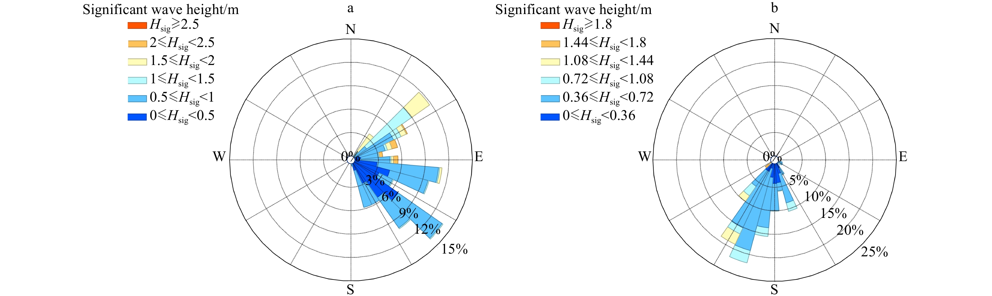
Figure 7. Wave rose diagrams in winter (a) and summer (b) in the BG based on results of Exp. R2.
Figure 8. The Hsigdifference triggered by the currents (shaded color) under the winter southeast wave, results are derived from the outputs between the Exps. R4 and R3 (R4–R3), values below 5 cm are blanked, the purple arrows show the Hsig and wave direction based on Exp. R2, the green arrows show the surface current vectors based on Exp. R1.
Figure 9. Same as Fig. 8, but for the summer southwest wave case.
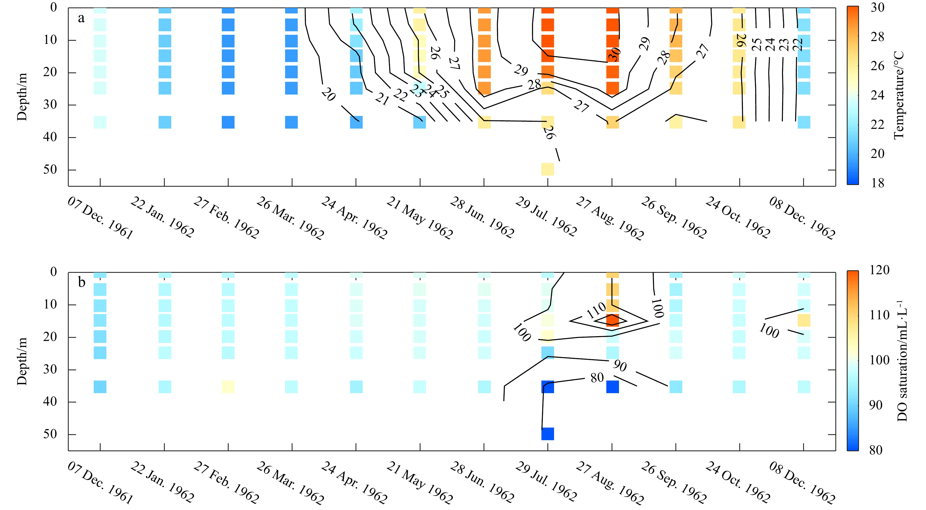
Figure 10. Time series of temperature (a) and dissolved oxygen (DO) saturation (b) profiles at Station 7204 (Fig. 1a) during the China General Oceanographic Survey.
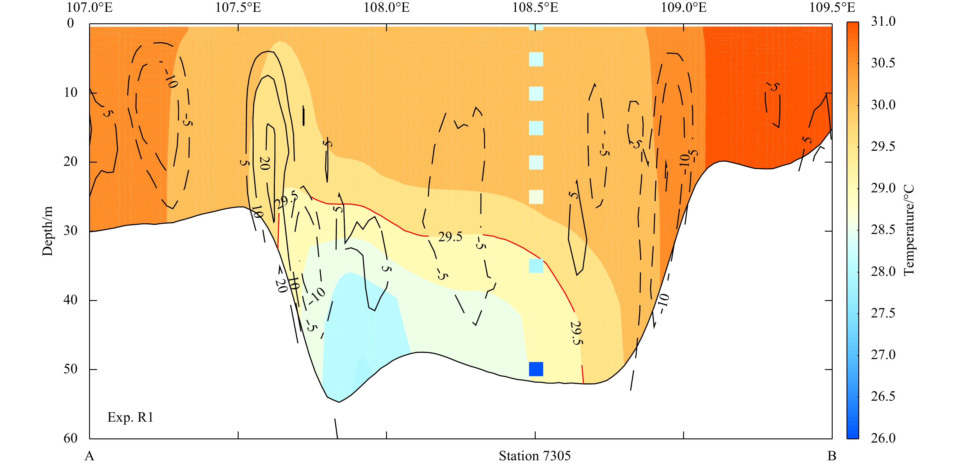
Figure 11. Monthly averaged temperature along Section AB (Fig. 1a) during June 2014; solid-black lines indicate upward vertical velocity while dashed lines indicate downward motion (10–6 m/s); the scattered squares show the temperature profile observed at Station 7305 (Fig. 1a) in June 1962 during the China General Oceanographic Survey, all the results are based on Exp. R1.
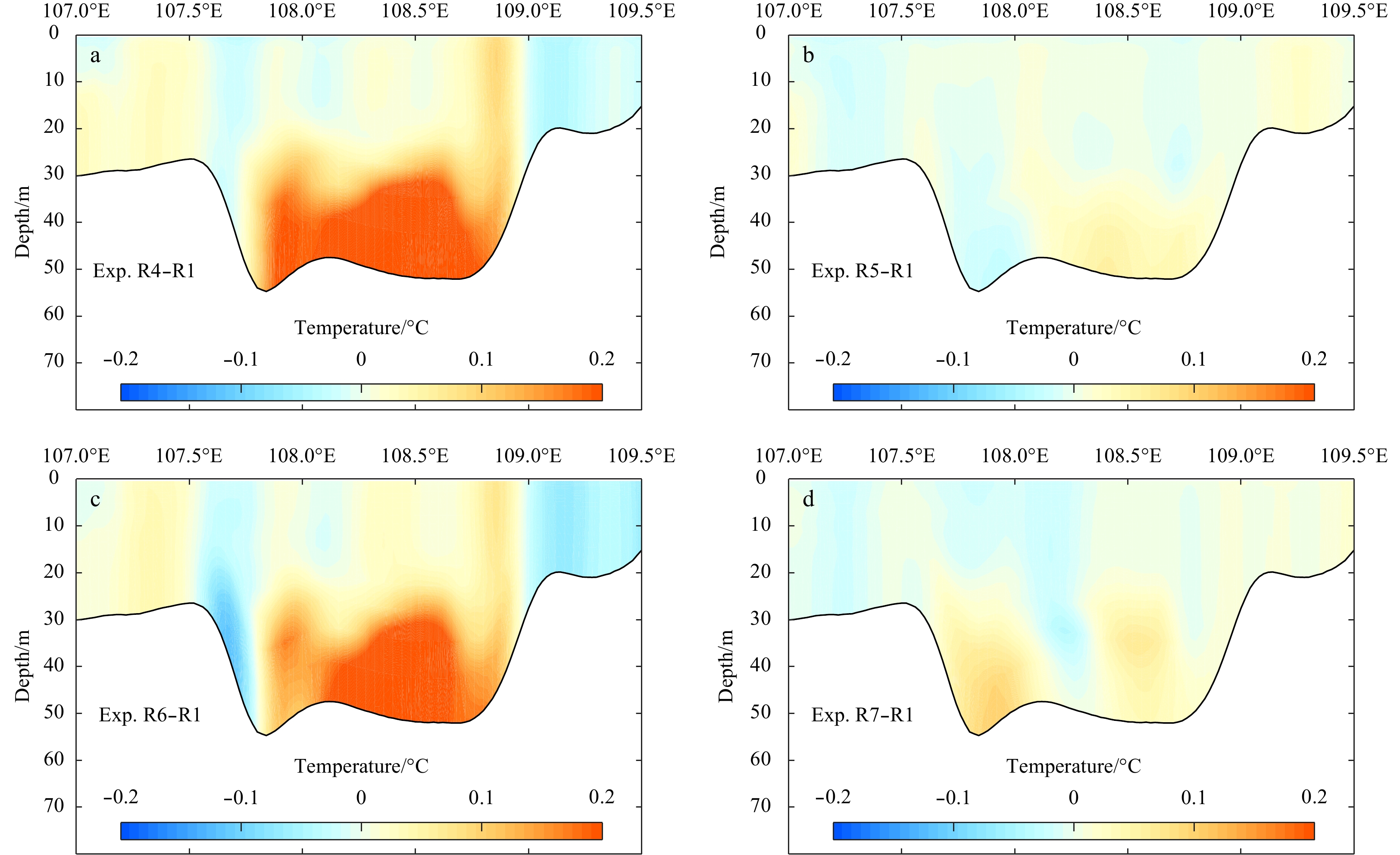
Figure 12. Temperature difference along Section AB between numerical experiments R4 and R1 (a), R5 and R1 (b), R6 and R1 (c), R7 and R1 (d).
Figure 13. The sea surface salinity superposed by the depth-averaged velocity in the top BG areas, the data is based on the monthly averaged outputs of Exp. R1 during June 2014.
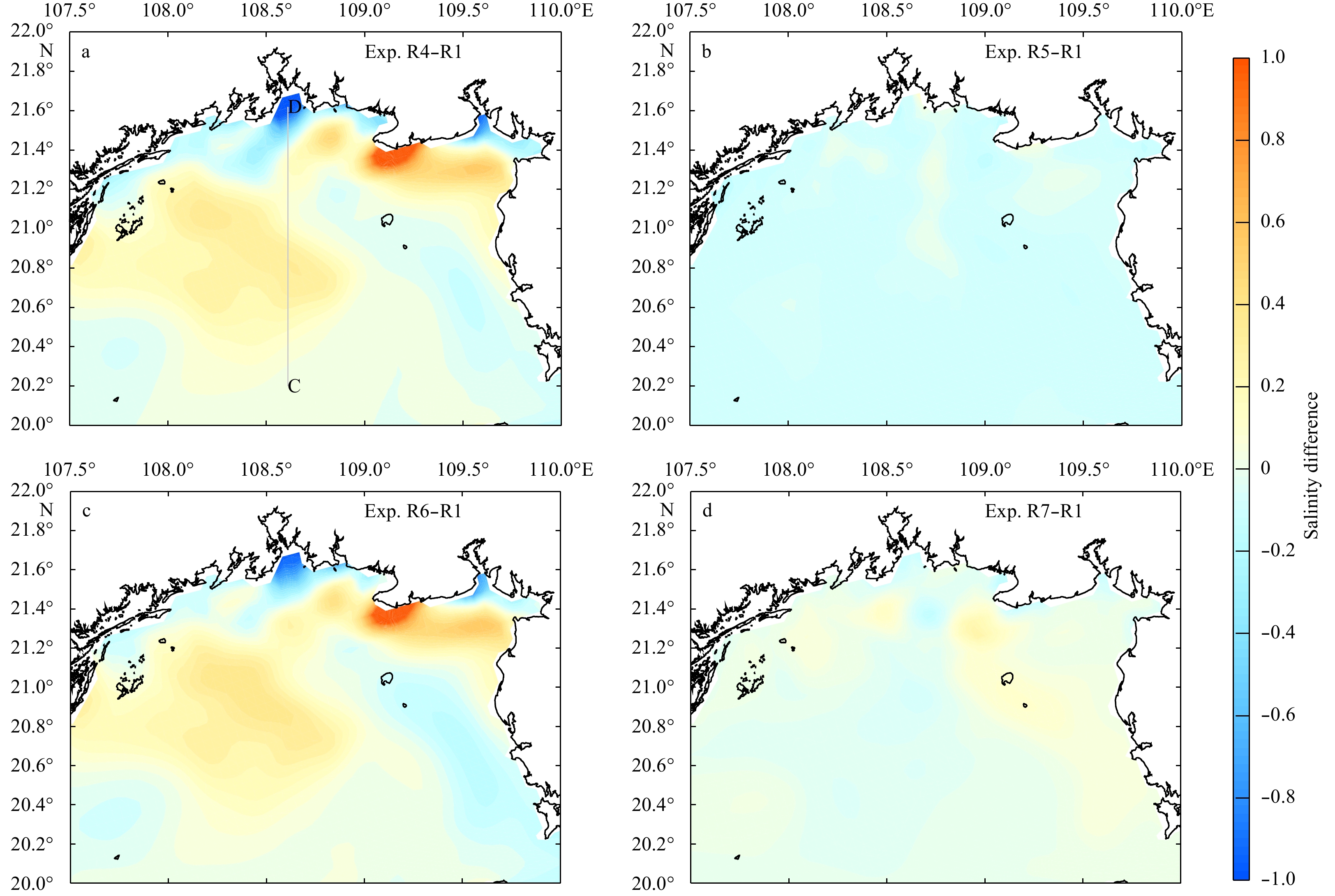
Figure 14. The sea surface salinity difference in the top BG areas between numerical experiments R4 and R1 (a), R5 and R1 (b), R6 and R1 (c), R7 and R1 (d).
Figure 15. The salinity difference along Section CD between numerical experiments R4 and R1 (a), R5 and R1 (b), R6 and R1 (c), R7 and R1 (d).
Figure 16. The streamline of depth-averaged flow during June, 2014 based on the monthly-averaged data from Exp. R1, the black box shows the BGCWM domain.
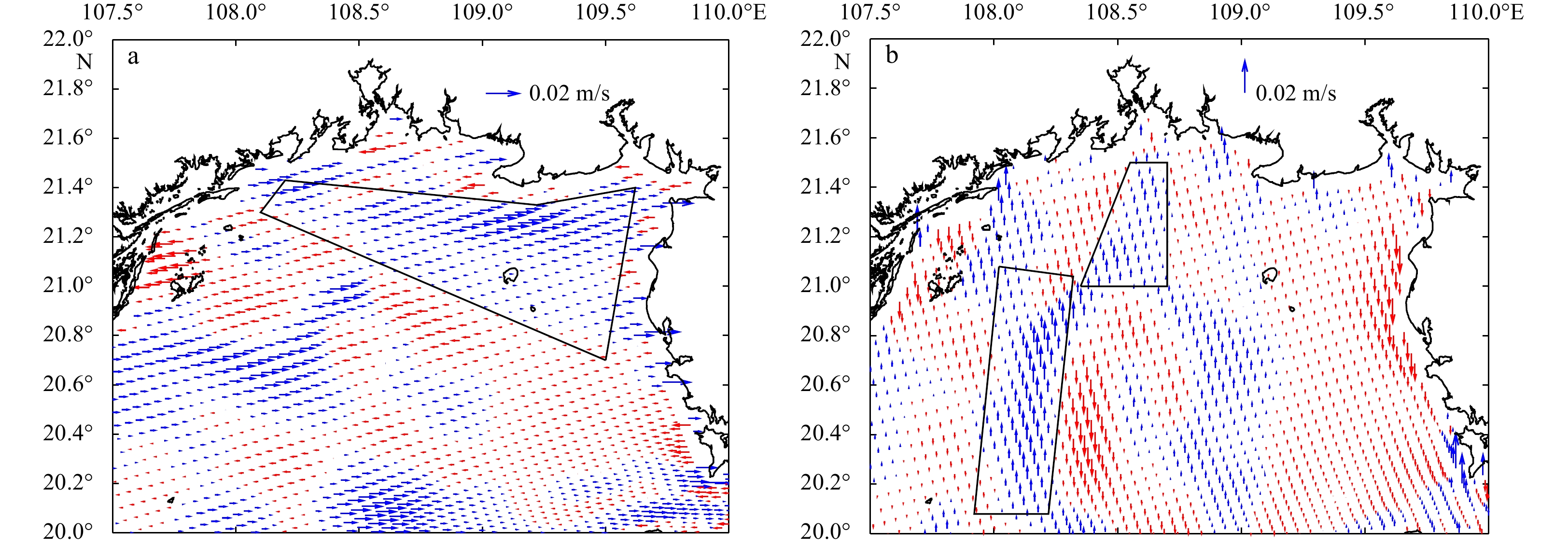
Figure 17. Difference of monthly mean depth-averaged flow between Exp. R4 (a), R5 (b), R6 (c), R7 (d) and the R1 during June 2014. Arrows show changes of the current vectors, colors display changes of the magnitude for the current, with positive value indicating the current is enhanced and vice versa. Black box shows the BGCWM domain and the red line shows the location of Section EF.
Figure 18. Differences of eastward (a) and northward (b) current components of the monthly mean depth-averaged flow in June 2014 between Exps. R6 and R1 (R6–R1), where blue arrows indicating negative values and red arrows for positive ones.


 DownLoad: