


Figure
1.
Typical SAR ISW Images obtained from Sentinel-1 (a–c) and GF-3 (d–f).
| Citation: | CHOI Youngjin. Comparative simulation study of effects of eddy-topography interaction in the East/Japan Sea deep circulation[J]. Acta Oceanologica Sinica, 2015, 34(7): 1-18. doi: 10.1007/s13131-015-0693-1

|
The Malacca Strait with 1 080 km long is the most important energy transport route. Due that the internal solitary waves (ISWs) have great influence on the navigation of ships and submarines, especially, Malacca Strait is the area where the ISWs occur frequently, it is necessary to study the characteristics of the ISWs in Malacca Strait.
It is well known that ISWs phenomenon shows strong randomness, and its amplitude, propagation velocity and wavelength are greatly affected by hydrology and other external environment (Fang and Du, 2005; Li et al., 2013; Alford et al., 2010; Cai and Xie, 2010; Huang et al., 2007; Hyder et al., 2005; Lai et al., 2010). The research of ISWs based on SAR image usually includes the following two aspects. One is to study the temporal and spatial distribution of ISWs. For example, in 2000, Hsu et al. (2000) studied the distribution of ISWs in the South China Sea based on 5-year satellite remote sensing images. Using satellite SAR data from July to October 2007, Kozlov et al. (2015) studied the characteristics of short-period ISWs in the Kara Sea. Filonov et al. (2014) studied the spatial distribution of ISWs of Todos Santos by means of the combination of real measurement and remote sensing. Another one is the imaging mechanism of ISWs on SAR image and the inversion of ISWs parameters. For example, in 2013, Liu et al. (2013) calculated the nonlinear phase velocity of the ISWs in the South China Sea using multi-source remote sensing data, and found that the velocity of the ISWs was greatly affected by the depth of water. In 2016, combined with nonlinear Schrodinger (NLS) equation, our team obtained the inversion model of SAR ISWs parameters, and the inversion results are close to the measured data (Zhang et al., 2016). With the increasing number of satellites in orbit, the understanding of ISWs by multi-source remote sensing becomes to be more and more comprehensive (Jackson, 2007; Schuler et al., 2003).
In a word, there is no research on the ISWs in Malacca Strait up to date. In this paper, ISWs in Malacca Strait are investigated from the spatial distribution of the waves, the velocity and amplitude of the ISWs, and so on, which will provide valuable scientific references for maritime navigation and marine engineering.
The Malacca Strait is located in the region of 0°–6°N and 97°–104°E. In order to observe and analyze the characteristics of ISWs in the Malacca Strait, Sentinel-1 SAR data from June 2015 to December 2016 and GF-3 data from April 2018 to March 2019 are collected. Because of the limitation of SAR orbital period, we obtain 20 Sentinel-1 images and 24 GF-3 images in total, and 344 ISW packets and ISWs are collected.
It can be seen from Fig. 1 that the ISWs in the Malacca Strait mainly appear in the form of wave packets and single solitary waves. Though the direction of ISWs propagation seems to be very complex, however, it always tends to propagate towards the shore.
Furtherly, according to the position and the crest length of the leading wave in the ISW packets in 45 SAR images, the spatial distribution of the wave and the length distribution of the leading wave crest in the Malacca Strait are obtained, which are shown in Fig. 2 and Fig. 3, respectively. As shown in Fig. 2, in region A, the depth of water in this area is about 50–100 m, and the largest wave packets is observed, accompany with a relatively long crest length of the leading wave. In the middle of the Malacca Strait (region B), the water depth is about 20–50 m, the ISW propagates in the form of wave packets and single solitary waves, and the crest length of the leading wave becomes shorter. In the southeast of the Malacca Strait (region C), the water depth is relatively shallow, with the shallowest part of only 4 m, and the ISW is mostly in the form of wave packets and single solitary waves, with the shortest crest length of the leading wave, but it is noticing that the ISWs is broken seriously, and the direction of the ISWs is also relatively messy.


By observed from satellite images, it can be found that there are three to seven ISWs on average in the Malacca Strait, with a maximum of 12 ISWs. The maximum (minimum) crest length of the wave packet is about 39 km (1.5 km) in the Fig. 2, and the crest length of the leading wave becomes to be shorter and shorter towards the southeast. Totally, 344 crest length of the leading wave are observed, in which 35 lines are more than 20 km in length, and most of them are located in the northwest region. In addition, most crest length of the leading wave less than 20 km are located in the regions B and C, and the number of crest length of the leading wave from 4 km to 14 km is about 273 crest lines, which accounts for the vast majority of total lines.
In addition, the occurrence of ISWs has a great relationship with seasons. Figure 4 shows the distribution of ISWs in different seasons. The largest number of ISWs observed from remote sensing images occurred from January to march, and the smallest from October to December. Most of the ISWs observed in SAR images from April to September occurred in region C.

The inversion of the ISWs parameters greatly depends on the two layer stratification. Temperature, salt and density data of the studied area are selected from the annual average data of World Ocean Atlas (2013), and hierarchical information is obtained by calculating the vertical distribution. The calculated temperature, salinity, density and buoyancy frequency curve are showed in Fig. 5. The water depth corresponding to the inflection point of buoyancy frequency in Fig. 5d is the upper water depth, about 25 m. The density corresponding to the upper water depth is found in the density curve, and the upper and lower average densities are calculated as 1 019.9 kg/m3 and 1 020.9 kg/m3 respectively.

Because of the balance between nonlinear effect and dispersion effect, the ISWs can be stable and spread over long distance.
The ISWs propagation equation adopts NLS equation. Combined with the SAR imaging mechanism of the ISWs, the amplitude inversion model of the ISWs based on the SAR image is established (NLS equation) (Zhang et al., 2016).
| $$\left\{ \begin{split} & D = 1.76l,\qquad \alpha \beta > 0\\ & D = 1.32l,\qquad \alpha \beta < 0 \end{split} \right.,$$ | (1) |
| $$\left\{ \begin{split} & {A_0} = \frac{{1.76}}{D}\sqrt {\left| {\frac{{2\alpha }}{\beta }} \right|},\qquad \alpha \beta > 0\\ & {A_0} = \frac{{1.32}}{D}\sqrt {\left| {\frac{{2\alpha }}{\beta }} \right|},\qquad \alpha \beta < 0 \end{split} \right.,$$ | (2) |
where A0 is the amplitude of the ISWs,
Then we apply the NLS amplitude inversion model to the previous 45 SAR images, and extract the distance D between the brightest spot and the darkest spot and hydrological parameters from each SAR image. The amplitude A0 of ISWs can be obtained from Eq. (2). We calculate the amplitude of ISWs happened in the Malacca Strait with water depth greater than 30 m.
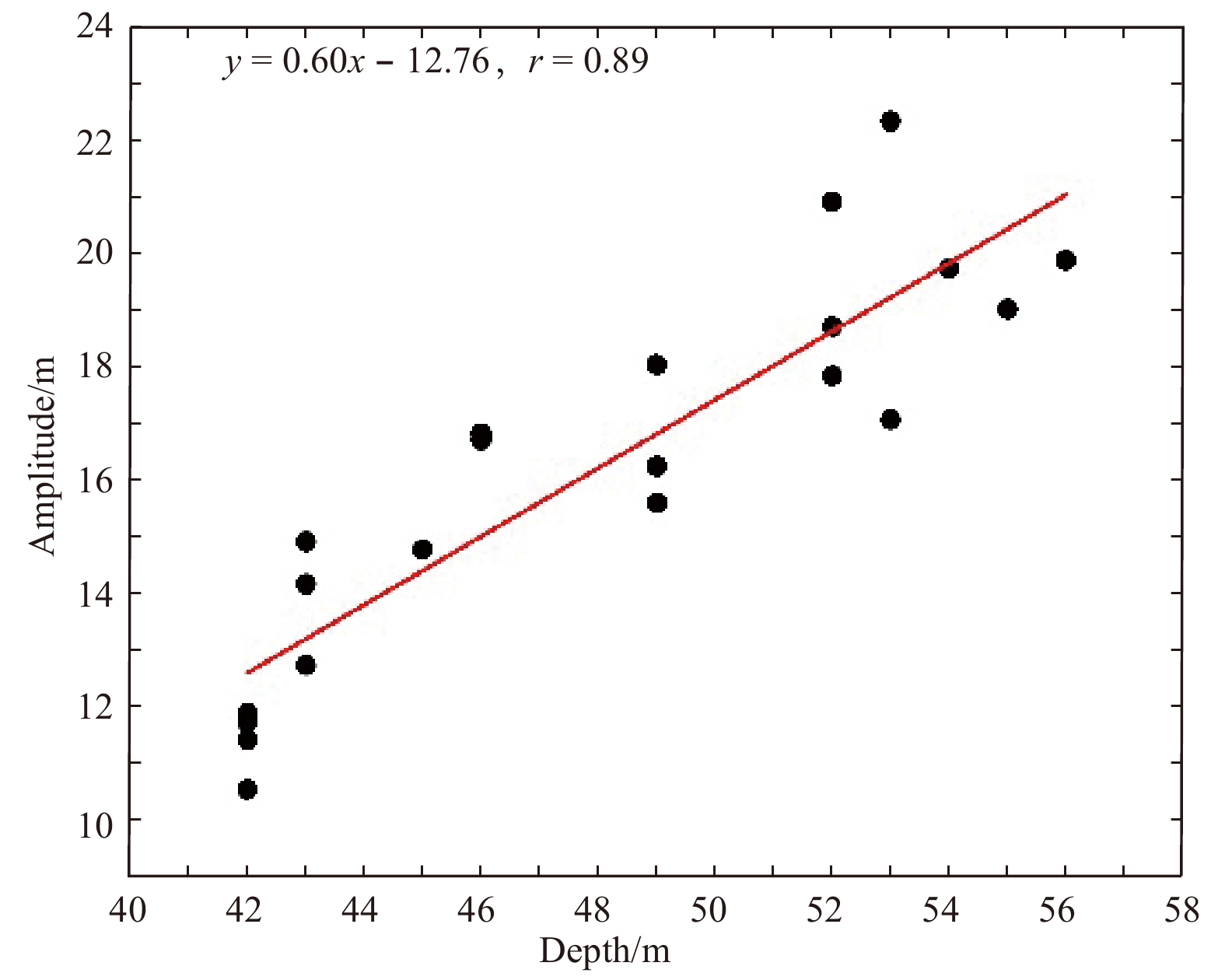
By extracting the characteristic parameters of ISWs in the Malacca Strait, the amplitude distribution is obtained, as shown in Fig. 6. In region A, the maximum amplitude obtained by NLS amplitude inversion model is 23.9 m, which is located at the water depth of 78 m, and the average amplitude of ISWs in this area is about 18.4 m. The maximum amplitude in region B calculated by NLS amplitude inversion model is 17.9 m, the minimum amplitude is 4.7 m, and the average amplitude of ISWs is about 10.9 m. The water depth in region C is shallow. The maximum and minimum amplitude calculated by NLS amplitude inversion model are 14.1 m and 4.7 m respectively, and the average amplitude is 9.6 m. In addition, we also analyze the amplitude of the one ISW. Figure 7 is a SAR image from March 14, 2016, we extracted the parameter and calculated the amplitude of ISWs. Each red dot in Fig. 7 is the extraction position of the ISWs parameter, combined with the local depth of water, the relationship between amplitude and depth of water is shown in Fig. 8. From Fig. 8, it can be found that even in the same ISW, the amplitude of ISWs is different, and the amplitude distribution is linearly related to the water depth. Figures 4 and 8 show that in Malacca Strait, with the decrease of water depth, the amplitude decreases. This may be due to the increase of the nonlinear effect of ISWs with the shallow water depth, which leads to the breakage of ISWs.

ISWs in the Malacca Strait can be divided into two types: single solitary waves and solitary wave packets. Therefore, we use NLS equation to derive the group velocity of solitary wave packets and KdV equation to obtain the phase velocity of single solitary waves.
The group velocity formula derived from the NLS equation (Zhang et al., 2015) is
| $${c_g} = \frac{{\rm d\omega }}{{\rm dk}} = \frac{\omega }{{2k}}\left[ {1 + \frac{{2k{h_2}}}{{ {\rm {sh}}(2k{h_2})}}} \right] ,$$ | (3) |
where k is the wave number, h2 is the depth of the lower layer, and
The phase velocity formula obtained by KdV equation (Zheng et al., 2001) is
| $$c = {\left[ {\frac{{g({\rho _2} - {\rho _1}){h_1}{h_2}}}{{{\rho _2}{h_1} + {\rho _1}{h_2}}}} \right]^{1/2}} + \frac{{\alpha {A_0}}}{3}, $$ | (4) |
where hl and h2 are the thickness of the upper and lower layers, respectively, and their water densities are
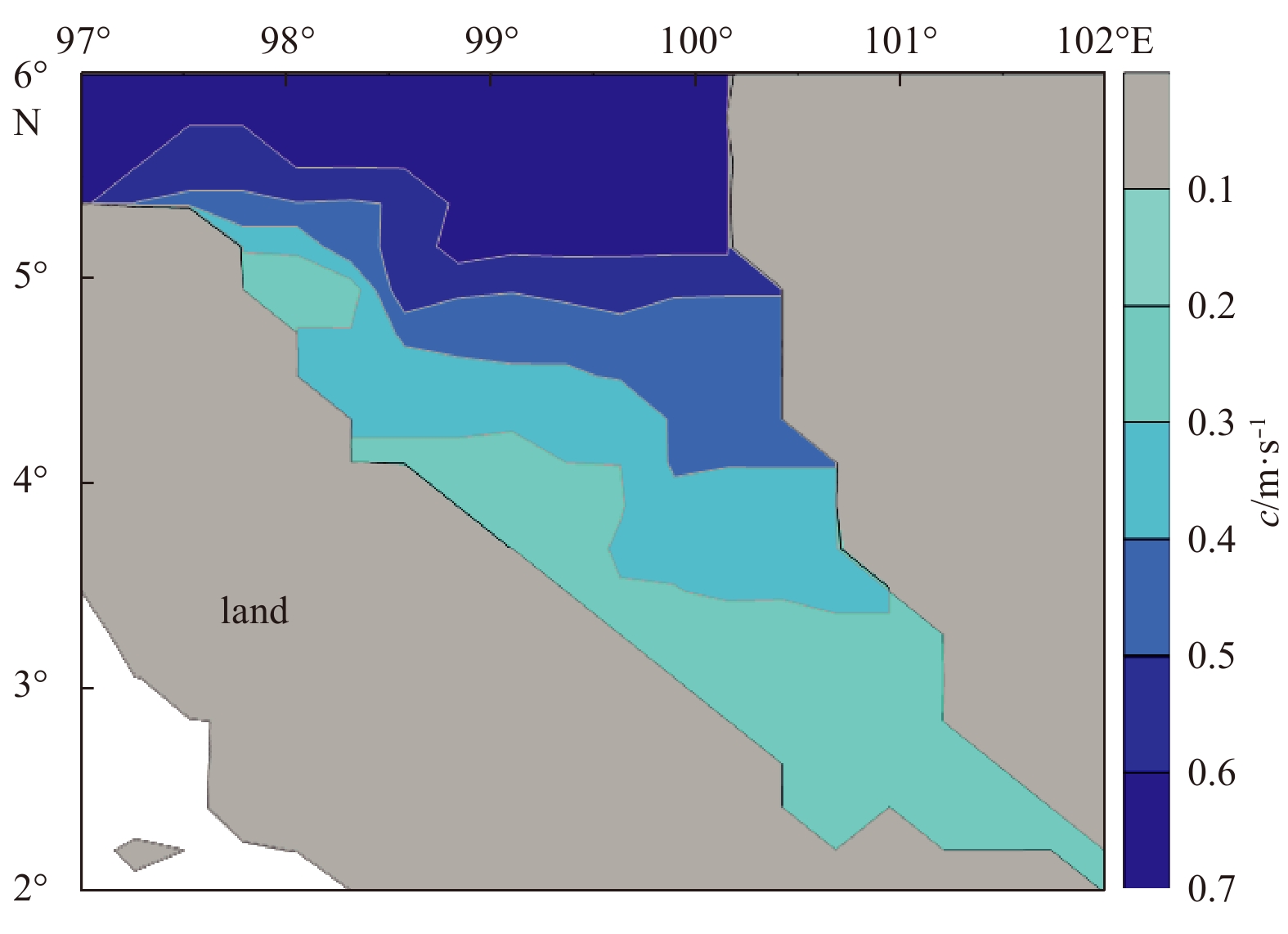
The propagation velocity of ISWs is affected by many factors, such as water depth, stratification. The two-dimensional water depth distribution map of Malacca Strait has been given in Fig. 2. It can be seen that the depth of the water in the south is the shallower, and the deeper is to the northwest. The distribution characteristics of the group velocity and the phase velocity in Malacca Strait are analyzed. Figure 9 shows the group velocity distribution of ISWs in Malacca Strait calculated by using the group velocity formula derived from the NLS equation. Figure 10 shows the distribution of phase velocity calculated by KdV equation.

As can be seen from Fig. 9, the group velocity of the wave packets reduced from 0.4 m/s to 0.12 m/s and the phase velocity of ISWs in Fig. 10 decreases from 0.6 m/s to 0.26 m/s. In general, the group velocity and phase velocity of ISWs in Malacca Strait are related to the topography.

Based on the Sentinel-1 and GF-3 SAR data, totally 45 SAR images in Malacca Strait are obtained, and the characteristic parameters of the ISWs in Malacca Strait are studied. The distribution of ISWs and crest length of the leading waves in Malacca Strait are statistically analyzed. It is found that ISWs are present in most of Malacca Strait, and the ISWs appear in the form of wave packets and single solitary waves. Furthermore, the direction of ISWs propagation is more complex, but the ISWs always tends to propagate towards the shore. The crest length of the leading wave is the longest in the northwest.
In addition, the group velocity and amplitude distributions of the area are calculated based on the high-order completely NLS equation inversion model. The phase velocity is obtained by KdV equation. The group velocity and phase velocity of ISWs are closely related to water depth and stratification. From northwest to southeast, with the water depth becoming shallow, the group velocity and phase velocity of ISWs becomes smaller. The group velocity distribution is between 0.12 m/s and 0.40 m/s, the phase velocity distribution is between 0.26 m/s and 0.6 m/s, and the amplitude of the ISWs is in the range of 4.7–23.9 m. The general trend of the amplitude and velocity is decreasing, which indicates that with the depth of water decreases, the nonlinearity increases, leading to the breakup of ISWs.
|
Chapman D C, Haidvogel D B. 1992. Formation of Taylor caps over a tall isolated seamount in a stratified ocean. Geophysical & Astrophysical Fluid Dynamics, 64(1-4): 31-65
|
|
Charney J G. 1947. The dynamics of long waves in a baroclinic westerly current. J Meteor, 4(5): 136-162
|
|
Choi B H, Kim K O, Eum H M. 2002. Digital bathymetric and topographic data for neighboring seas of Korea. J Korean Soc Coastal Ocean Eng (in Korean), 14: 41-50
|
|
Choi Y J, Yoon J-H. 2010. Structure and seasonal variability of the deep mean circulation of the East Sea (Sea of Japan). J Oceanogr, 66(3): 349-361
|
|
Crosby D S, Breaker L C, Gemmill W H. 1993. A proposed definition for vector correlation in geophysics: theory and application. J Atmos Oceanic Technol, 10(3): 355-367
|
|
Danchenkov M A, Riser S C, Yoon J-H. 2003. Deep currents of the central Sea of Japan. Pacific Oceanogr, 1: 6-11
|
|
Dewar W K. 1998. Topography and barotropic transport control by bottom friction. J Mar Res, 56: 295-328
|
|
Eady E T. 1949. Long waves and cyclone waves. Tellus, 1(3): 33-52
|
|
Eby M, Holloway G. 1994. Grid transformation for incorporating the Arctic in a global ocean model. Climate Dyn, 10(4-5): 241-247
|
|
Gent P R, McWilliams J C. 1990. Isopycnal mixing in ocean circulation models. J Phys Oceanogr, 20(1): 150-155
|
|
Greatbatch R J. 1998. Exploring the relationship between eddy-induced transport velocity, vertical momentum transfer, and the isopycnal flux of potential vorticity. J Phys Oceanogr, 28(3): 422-432
|
|
Greatbatch R J, Li Guoqing. 2000. Alongslope mean flow and an associated upslope bolus flux of tracer in a parameterization of mesoscale turbulence. Deep-Sea Res Pt I, 47(4): 709-735
|
|
Hanawa K, Mitsudera M. 1985. About constructing of daily mean values of ocean data. Coastal Res Note, 23: 79-87
|
|
Hirose N, Kawamura H, Lee H J, et al. 2007. Sequential forecasting of the surface and subsurface conditions in the Japan Sea. J Oceanogr, 63(3): 467-481
|
|
Hogan P J, Hurlburt H E. 2000. Impact of upper ocean-topographical coupling and isopycnal outcropping in Japan/East Sea models with 1/8°to 1/64°resolution. J Phys Oceanogr, 30(10): 2535- 2561
|
|
Holloway G. 1992. Representing topographic stress for large-scale ocean models. J Phys Oceanogr, 22(9): 1033-1046
|
|
Holloway G. 2008. Observing global ocean topostrophy. J Geophys Res, 113(C7): C07054, doi: 10.1029/2007JC004635
|
|
Holloway G, Sou T, Eby M. 1995. Dynamics of circulation of the Japan Sea. J Mar Res, 53(4): 539-569
|
|
Holloway G, Wang Zeliang. 2009. Representing eddy stress in an Arctic Ocean model. J Geophys Res, 114: C06020, doi: 10.1029/ 2008JC005169
|
|
Huppert H E. 1975. Some remarks on the initiation of inertial Taylor columns. J Fluid Mech, 67: 397-412
|
|
Ishizaki H, Motoi T. 1999. Reevaluation of the Takano-Oonishi scheme for momentum advection on bottom relief in ocean models. J Atmos Oceanic Technol, 16(12): 1994-2010
|
|
Isoda Y, Saitoh S I. 1993. The northward intruding eddy along the East coast of Korea. J Oceanogr, 49(4): 443-458
|
|
Kim Y J. 2007. A study on the Japan/East Sea oceanic circulation using an extra-fine resolution model [dissertation]. Fukuoka: Kyushu University
|
|
Kim K, Kim K-R, Kim D-H, et al. 2001. Warming and structural changes in the East (Japan) Sea: A clue to future changes in global oceans? Geophys Res Let, 28(17): 3293-3296
|
|
Kim C H, Yoon J-H. 1996. Modeling of the wind-driven circulation in the Japan Sea using a reduced gravity model. J Oceanogr, 52(3): 359-373
|
|
Kitani K. 1987. Direct current measurement of the Japan Sea Proper Water (in Japanese). Nihonkai-ku Suisan Shiken Kenkyuu Renraku News, Japan Sea National Fisheries Research Institute, 341: 1-6
|
|
Lee H J, Yoon J-H, Kawamura H, et al. 2003. Comparison of RIAMOM and MOM in modeling the East Sea/Japan Sea circulation. Ocean and Polar Research, 25(3): 287-302
|
|
Luchin V A, Manko A N, Mosyagina S Y, et al. 2003. Hydrography of water masses (in Russian). In: Terziev F S, ed. Hydrometeorology and Hydrochemistory of Seas. Sankt-Petersburg: Hydrometeoizdat, 8: 157-256
|
|
Maltrud M, Holloway G. 2008. Implementing biharmonic neptune in a global eddying ocean model. Ocean Modelling, 21(1-2): 22-34
|
|
Merryfield W, Scott R. 2007. Bathymetric influence on mean currents in two high-resolution near-global ocean models. Ocean Modelling, 16(1-2): 76-94
|
|
Mesinger F, Arakawa A. 1976. Numerical methods used in atmospheric models, Volume 1. WMO/ICSU Joint Organizing Committee, GARP Publication Series No. 17
|
|
Minobe S, Sako A, Nakamura M. 2004. Interannual to interdecadal variability in the Japan sea based on a new gridded upper water temperature dataset. J Phys Oceanogr, 34(11): 2382-2397
|
|
Mori K, Matsuno T, Senjyu T. 2005. Seasonal/spatial variations of the near-inertial oscillations in the deep water of the Japan Sea. J Oceanogr, 61(4): 761-773
|
|
NCAR. 1989. NCAR ASCII Version of ETOPO5 earth surface elevation. Data Support Section, NCAR
|
|
Noh Y. 1996. Dynamics of diurnal thermocline formation in the oceanic mixed layer. J Phys Oceanogr, 26(10): 2183-2195
|
|
Oort A H, Ascher S C, Levitus S, et al. 1989. New estimates of the available potential energy in the World Ocean. J Geophys Res, 94(C3): 3187-3200
|
|
Penduff T, Juza M, Brodeau L, et al. 2010. Impact of global ocean model resolution on sea-level variability with emphasis on interannual time scales. Ocean Sci, 6: 269-284
|
|
Sakai R, Yoshikawa Y. 2005. Numerical experiments on the formation mechanism of abyssal current in the Japan Sea. Engineer Sci Rep Kyushu Univ (in Japanese), 26(4): 423-430
|
|
Salmon R, Holloway G, Hendershott M C. 1976. The equilibrium statistical mechanics of simple quasi-geostrophic models. J Fluid Mech, 75(4): 691-703
|
|
Senjyu T, Shin H R, Yoon J-H, et al. 2005. Deep flow field in the Japan/East Sea as deduced from direct current measurements. Deep-Sea Res Pt II, 52(11-13): 1726-1741
|
|
Senjyu T, Sudo H. 1996. Interannual variation of the upper portion of the japan sea proper water and its probable cause. J Oceanogr, 52(1): 27-42
|
|
Seung Y-H, Yoon J-H. 1995. Robust diagnostic modeling of the Japan sea circulation. J Oceanogr, 51(4): 421-440
|
|
Shin H R, Shin C W, Kim C, et al. 2005. Movement and structural variation of warm eddy WE92 for three years in the Western East/Japan Sea. Deep-Sea Res Pt II, 52(11-13): 1742-1762
|
|
Takano K. 1974. A General Circulation Model For the World Ocean. Numerical Simulation of Weather and Climate Technical Report. Los Angeles: Univ of California, 47
|
|
Takematsu M, Nagano Z, Ostrovski A, et al. 1999. Direct measurements of deep currents in the northern Japan Sea. J Oceanogr, 55(2): 207-216
|
|
Takikawa T, Yoon J-H. 2005. Volume transport through the Tsushima straits estimated from sea level difference. J Oceanogr, 61(4): 699-708
|
|
Taylor G I. 1917. Motion of solids in fluids when the motion is not irrotational. Proc Roy Soc, A93: 99-113
|
|
Teague W J, Tracey K L, Watts D R, et al. 2005. Observed deep circulation in the Ulleung Basin. Deep-Sea Res Pt II, 52(11-13): 1802-1826
|
|
Wallcraft A J, Kara A B, Hurlburt H E. 2005. Convergence of Laplacian diffusion versus resolution of an ocean model. Geophys Res Lett, 32(7), doi: 10.1029/2005GL022514
|
|
Webb D J, de Cuevas S J, Richmond C S. 1998. Improved advection schemes for ocean models. J Atmos Oceanic Technol, 15(5): 1171-1187
|
|
Wessel P, Smith W H F. 1998. New, improved version of generic mapping tools released. EOS Trans AGU, 79: 579
|
|
Yoon J-H, Kawamura H. 2002. The formation and circulation of the intermediate water in the Japan Sea. J Oceanogr, 58(1): 197-211
|


Supported by:
Beijing Renhe Information Technology Co. Ltd


 DownLoad:


