

-
Abstract: Marine Heatwave (MHW) events refer to periods of significantly elevated sea surface temperatures (SST), persisting from days to months, with significant impacts on marine ecosystems, including increased mortality among marine life and coral bleaching. Forecasting MHW events is crucial to mitigate their harmful effects. This study presents a two-step forecasting process: short-term SST prediction followed by MHW event detection based on the forecasted SST. Firstly, we developed the “SST-MHW-DL” model using the ConvLSTM architecture, which incorporates an attention mechanism to enhance both SST forecasting and MHW event detection. The model utilizes SST data from the preceding 60 days to forecast SST and detect MHW events for the subsequent 15 days. Verification results for SST forecasting demonstrate a Root Mean Square Error (RMSE) of 0.64℃, a Mean Absolute Percentage Error (MAPE) of 2.05%, and a coefficient of determination (R²) of 0.85, indicating the model’s ability to accurately predict future temperatures by leveraging historical sea temperature information. For MHW event detection using forecasted SST, the evaluation metrics of “accuracy,” “precision,” and “recall” achieved values of 0.77, 0.73, and 0.43, respectively, demonstrating the model’s capability to capture the occurrence of MHW events accurately. Furthermore, the attention-enhanced mechanism reveals that recent SST variations within the past 10 days have the most significant impact on forecasting accuracy, while variations in deep-sea regions and along the Taiwan Strait significantly contribute to the model’s efficacy in capturing spatial characteristics. Additionally, the proposed model and temporal mechanism were applied to detect MHWs in the Atlantic Ocean. By inputting 30 days of SST data, the model predicted SST with an RMSE of 1.02℃ and an R² of 0.94. The accuracy, precision, and recall for MHW detection were 0.79, 0.78, and 0.62, respectively, further demonstrating the model’s robustness and usability.
-
1. Introduction
Persistent and significant increases in Sea Surface Temperature (SST) have far-reaching implications for global climate, marine ecosystems, and human societies. Internationally, episodes of exceptionally high ocean temperatures lasting for at least five days are categorized as marine heatwave (MHW) events (Oliver et al., 2018). These MHW events have profound impacts on marine biodiversity, fisheries, and aquaculture, resulting in widespread biological mortality, disease outbreaks, coral bleaching, and depletion of seagrass (Smith et al., 2021; Claar and Wood, 2020; Lian and Gao, 2024). Consequently, the study of MHWs is of critical theoretical importance and plays a central role in diverse economic activities.
As global warming persists, the frequency and intensity of MHW are likely to escalate further (Frölicher et al., 2018). Detecting and predicting these heatwave events have become a key focus of current research efforts. Currently, two main methodologies for forecasting heatwaves prevail: dynamic models and artificial intelligence (AI) models. Dynamic models, derived from physical and numerical weather forecasts, simulate and predict MHW occurrences by controlling various parameters that influence oceanic SST, such as heat fluxes, sea level pressure, and wind speed (Hu and Li, 2022; Yu et al., 2024). In contrast, recently developed AI models employ data-driven forecasting, typically using SST data or heatwave datasets. While dynamic models have garnered significant attention for forecasting MHWs, most studies have concentrated on longer timescales (annual, seasonal, or monthly), resulting in a relative scarcity of short-term forecasts spanning one to two weeks. For example, Hövel et al. (2022) assessed the predictability of MHWs over the past decade using the Max Planck Earth System Model, focusing on the temporal and frequency characteristics of MHWs in the North Atlantic region, achieving forecasts up to eight years in advance. De Burgh-Day et al. (2022), employing the ACCESS-S1 model, conducted heatwave forecasting and assessment in three key aquaculture regions surrounding New Zealand, demonstrating the model’s ability to predict heatwave events in these regions up to two months in advance.
In recent years, the rapid advancement of AI technology in oceanography has sparked increasing interest in heatwave research based on AI methodologies. Two primary approaches have emerged: the first directly forecasts future heatwave events based on historical heatwave data, using a phenomenon-based prediction from past “heatwaves” to future occurrences. However, this method is still in its infancy and currently demonstrates limited accuracy. The second approach breaks down heatwave prediction into two stages: initially forecasting SST and then utilizing the forecasted SST data for heatwave detection. Over the past decade, SST forecasting has progressed to a relatively mature stage. Techniques such as Convolutional Neural Networks (CNN), (Han et al., 2019) and Recurrent Neural Networks (RNN), (Jahanbakht et al., 2022) for SST prediction have shown effectiveness in short-term forecasts (less than 7 days) (Zhang et al., 2020, 2022). Nonetheless, marine heatwave events often persist for more than 5 days, with some lasting several weeks, posing a challenge for accurate prediction beyond one week. Moreover, most SST forecasting studies have inadequately explored the relationship between historical data length and the duration of future forecasts. Determining the necessary historical data length for forecasting models often relies on empirical methods or multiple experiments. For example, Giamalaki et al. (2022) utilized a random forest model to analyze heatwave events in the Northeast Pacific, achieving 76% accuracy within a one-week forecasting period. However, when predicting severe heatwave events extending beyond 10 days, the overall accuracy substantially decreased to 38%.
The objectives of this paper are as follows: 1) to introduce a deep learning model trained on comprehensive historical SST data to effectively forecast SST beyond two weeks using a restricted amount of historical SST data, and subsequently utilize the forecasted SST data to identify MHW events, thereby predicting heatwave occurrences; 2) to investigate the spatiotemporal correlations between historical and future SST using an attention mechanism, thus enhancing the proposed forecasting model’s understanding of the spatiotemporal characteristics of SST and heatwaves; and 3) to conduct experiments in new regions to determine the effectiveness of the proposed model and temporal mechanism, aiming to better validate the proposed approach.
2. Study area and data
2.1 Study Area
This study focuses on the East China Sea (ECS), a region frequently affected by MHWs, spanning from 23°N to 35°N and 117°E to 132°E. MHWs in this area have increased harmful algal blooms, shifted marine species northward, and exacerbated hypoxia and acidification, significantly impacting biodiversity, fisheries, and ecosystem services (Wang et al., 2023a). As is shown in Fig. 1, much of this region features sea depths not exceeding
1000 meters, exhibiting substantial fluctuations in SST and pronounced seasonal variability (>1℃/month). The SST changes in the ECS are significantly influenced by coastal tidal systems and complex circulation patterns such as the Kuroshio Current (Wei et al., 2023), the Taiwan Warm Current (Lee et al., 2021), and the coastal currents along the ECS (Cao et al., 2021). Situated within the subtropical zone, the average annual water temperature of the ECS ranges between 20℃ to 24℃, with yearly temperature variations fluctuating between 7℃ to 9℃. As one of China’s proximate maritime regions, the ECS has abundant fishery resources and ranks among China’s most productive sea areas (Wang et al., 2023c). Figure 1. Study area. (a) Topography of the ECS and its primary ocean currents, (b) SST variations in the ECS from 2016 to 2021.
2.2 Data used
The SST data utilized in this study is sourced from the Optimum Interpolation Sea Surface Temperature (OISST) dataset curated by the National Oceanic and Atmospheric Administration (NOAA). The OISST dataset is a spatially gridded amalgamation derived by interpolating and integrating SST observations acquired from satellite and in-situ measurements, including data from ship surveys and buoys. Characterized by a daily temporal resolution and a spatial resolution of 0.25°, this dataset spans from September 1, 1981, to the current day. It is an extensively employed reanalysis data products in the field of MHW research (Fredston et al., 2023; Iskandar et al., 2021). In this study, data spanning from 1981 to 2015 has been allocated for training and validation, while the remaining data spanning from 2016 to 2021 was used for testing. The SST data was normalized to optimize its distribution, improving model training efficiency and convergence.
3. Methodology
3.1 Marine Heatwaves' Definitions
The definition of MHW was initially introduced by Pearce et al. (2011) to describe events of abnormally warm water that significantly impact marine ecosystems. Various definitions of MHWs are currently in use, as illustrated in Fig. 2, where the blue lines represent climatological temperatures based on a 30 years baseline period (1981–2010), and the green line represents the threshold for MHW.
 Figure 2. Different methods for MHW detection.
The Fixed Threshold Method (Fig. 2a) defines MHWs based on the absolute temperature of the annual maximum temperature (green dashed line) or a fixed percentile threshold (green solid line) (Oliver et al., 2021). This method is effective in detecting events during warm seasons but may produce anomalous results in other seasons. For instance, using a fixed threshold might miss significant events during cooler seasons or overemphasize events during warmer seasons.
The Seasonal Percentile Threshold Method (Fig. 2b), proposed by Hobday et al. (2016), uses the 90th percentile of sea temperatures during the climatological reference period (1981-2010) to detect MHWs in both warm and cool seasons. An event is recognized as an MHW if the current SST remains above this threshold for at least five consecutive days. This method ensures that heatwaves are detected year-round and accounts for seasonal variations.
The Elevated Threshold Method (Fig. 2c) uses higher percentiles to isolate the most extreme events, focusing on the more severe occurrences (Shanks et al., 2020). For example, setting the threshold at the 95th or 99th percentile can help identify only the most intense heatwaves, resulting in fewer but more extreme events being classified as MHWs. This method is useful for studying the impacts of the most severe warming events.
The Threshold Classification Scheme (Fig. 2d) allows for different lower percentile thresholds to accommodate various research needs (Hobday et al., 2018). For example, different percentiles can be set for different regions or times of the year to better capture regional and temporal variations in MHWs. This method provides flexibility in defining heatwaves according to specific research goals.
From Fig. 2, it is evident that different definitions result in varying numbers of heatwave events. Compared to Fig. 2a, Figs. 2b and d show more frequent heatwave events, while Fig. 2c shows fewer, shorter-duration events representing the most extreme heatwaves. The seasonal percentile threshold method (Fig. 2b) results in more widespread detection of heatwaves, making it the most commonly used approach (Smith et al., 2023; Bian et al., 2023). Therefore, this study adopts the seasonal percentile threshold method (Fig. 2b), where the 90th percentile of sea temperature during the climatological reference period (1981-2010) serves as the threshold for MHWs. An event is recognized as an MHW if the current SST remains above this threshold for at least five consecutive days, indicating an abnormal warming event. Furthermore, this method defines MHW intensity as the difference between the temperature peak and the climatological temperature derived from the average SST based on the 1981-2010 OISST/SST data.
3.2 The proposed SST-MHW-DL model
To better capture the spatiotemporal characteristics of SST fields and effectively detect MHWs, we propose a deep learning model termed the “SST-MHW-DL Network Model” (Fig. 3a). This model is based on the Convolutional Long Short-Term Memory (ConvLSTM) architecture and enhanced with the Convolutional Block Attention Module (CBAM) (Woo et al., 2018). The ConvLSTM combines the features of CNN and LSTM structures, showcasing exceptional capabilities in sequence modeling and sensitivity to spatial information (Shi et al., 2015). It effectively captures long-term dependencies within sequential data, making it suitable for spatiotemporal sequence modeling and forecasting. The CBAM introduces “channel attention” and “spatial attention” mechanisms within the CNN, significantly improving the model’s perception and learning capabilities concerning the spatiotemporal features of SST. The “channel attention” emphasizes essential temporal features within the input SST data, while the “spatial attention” highlights critical spatial regions within the SST image. The integration of these mechanisms enhances the heatwave forecasting model’s ability to perceive historical SST temporal features and crucial spatial SST regions.
 Figure 3. Structural diagram of the proposed SST-MHW-DL model (the red box highlights our improvement and analysis part).
The proposed model comprises six pivotal layers shown in Fig. 3a: the SST input layer, the CBAM module layer, three ConvLSTM layers, the output layer, and the heatwave detection layer. Notably, the CBAM module can be attached before each ConvLSTM layer; however, for a deeper investigation into the spatiotemporal correlation between historical and future SST, this study chose to place the CBAM module at the initial position within the ConvLSTM network structure. The SST-MHW-DL model initially takes the input of SST data from the preceding 60 days. After processing by the CBAM-enhanced ConvLSTM module, it forecasts SST data for the forthcoming 15 days. Subsequently, utilizing the forecasted SST data, the model determines the occurrence of heatwave events in the research area via the heatwave detection module.
In the heatwave detection module, we experimented with several semantic segmentation models, such as U-Net and SegNet, using the predicted SST as input to capture temperature anomalies. However, the results showed that these complex models performed significantly worse in terms of accuracy, precision, and recall compared to the statistical methods proposed by Hobday et al. Moreover, the heatwave labels used in this study were also derived from the method of Hobday et al., reinforcing the close link between SST anomalies and MHWs. Given that more complex models did not provide substantial performance improvements, we determined that continuing with established, validated traditional methods is the most suitable approach in this context.
To evaluate the performance of the proposed SST-MHW-DL model, we compared it with several other models, including the basic ConvLSTM model (without attention enhancement), the Multi-Attention ConvLSTM model, and the U-Net model. The U-Net model is a well-known deep learning model extensively used in various prediction tasks and has demonstrated notable prediction results (Wang et al., 2023b; Ren and Li, 2023; Wang and Li, 2024).
3.3 Ground Truth Construction for training deep-learning model
This study used the historical SST dataset to generate ground-truth samples for training and validating the SST-MHW-DL model. As shown in Fig. 4, it randomly selected the SST data for 60 days and their corresponding adjacent 15 days to form ground-truth sample pairs. Each sample pair comprises historical SST, predicted SST, and its respective heatwave label (labeled "1" if the predicted SST is detected as a heatwave and "0" if not). The data from 1981 to 2015 were allocated for the training set (
10000 samples) and the validation set (2540 samples), while the data spanning from 2016 to 2021 was used for the testing set (2117 samples). Figure 4. Schematic representation of ground truth generation.
3.4 Model Evaluation
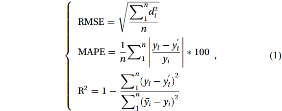
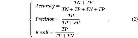
The performance of the SST-MHW-DL model for SST field prediction and MHW detection was evaluated carefully using a set of metrics. Three metrics were first used for assessing the accuracy of SST field prediction: root mean square error (RMSE), mean absolute percentage error (MAPE), and coefficient of determination (R²), as shown in Eq. (1). Additionally, three metrics—Accuracy, Precision, and Recall—were used to evaluate the accuracy of MHW detection shown in Eq. (2). Lower values of RMSE and MAPE indicate reduced errors in SST prediction, while an R² value closer to 1 signifies better alignment between the SST prediction result and actual data. Similarly, values approaching 1 for accuracy, precision, and recall denote a higher precision in MHW detection:
$$ \left\{\begin{array}{l}{\mathrm{RMSE}}=\sqrt{\dfrac{{\displaystyle\sum }_{1}^{n}{d}_{i}^{2}}{n}}\\ {\mathrm{MAPE}}=\dfrac{1}{n}{\displaystyle\sum }_{1}^{n}\left|\dfrac{{y}_{i}-{y}_{i}^{'}}{{y}_{i}}\right|*100\\ {\mathrm{R}}^{2}=1-\dfrac{{\displaystyle\sum }_{1}^{n}{({y}_{i}-{y}_{i}^{'})}^{2}}{{\displaystyle\sum }_{1}^{n}{(\bar{{y}_{i}}-{y}_{i})}^{2}}\end{array}{\mathrm{,}}\right. $$ (1) $$ \left\{\begin{array}{l} Accuracy=\dfrac{TN+TP}{TN+TP+FN+FP}\\ Precision=\dfrac{TP}{TP+FP}\\ Recall=\dfrac{TP}{TP+FN}\end{array}{\mathrm{,}}\right. $$ (2) where
$ {d}_{i} $ represents the difference between the labeled SST value$ {y}_{i} $ and the forecasted SST value$ {y}_{i}^{'} $ , and$ \bar{{y}_{i}} $ represents the mean value of the labeled SST, while n denotes the total number of testing samples. The FP (False Positive) represents cases where an MHW was not observed but was incorrectly detected by the model; TN (True Negative) represents scenarios where an MHW was neither observed nor detected by the model, indicating correct identification of the absence of an MHW event; FN (False Negative) represents instances of an MHW event; and TP (True Positive) represents instances where an actual MHW event was correctly detected by the model, indicating the successful identification of the presence of an MHW event.4. Results and discussion
4.1 Forecast SST
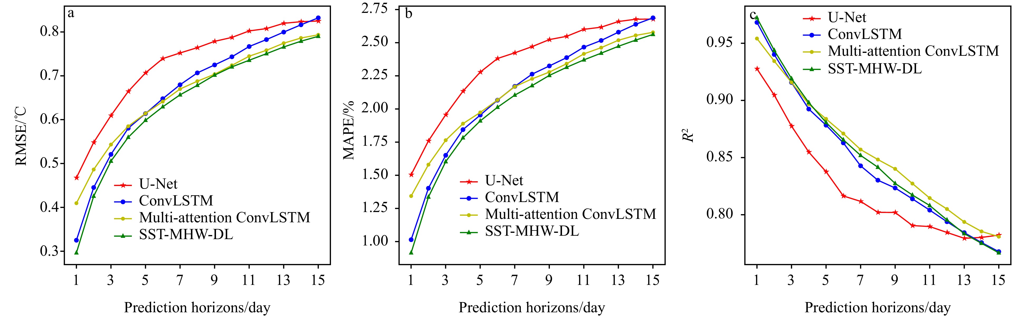
We conducted validation of the predictive performance of the SST-MHW-DL model within a 1−15 days forecasting period by calculating the RMSE, MAPE, and R² between the forecasted SST values and the ground-truth data. As shown in Fig. 5 and Table 1, the attention-enhanced SST-MHW-DL model demonstrated superior SST prediction accuracy compared to the basic ConvLSTM, as well as the U-Net and Multi-Attention ConvLSTM models. Additionally, we observed that as the forecast duration extended, the rate of error accumulation decelerated over time, indicating that the model has the potential to predict longer periods of time.
 Figure 5. SST forecast accuracy of the SST-MHW-DL model. a. RMSE. b. MAPE. c. R2.Table 1. Comparison of the proposed SST-MHW-DL with basic ConvLSTM, U-Net, and Multi-attention ConvLSTM models
Model RMSE/℃ MAPE/% R2 ConvLSTM 0.67 2.13 0.846 U-Net 0.73 2.35 0.823 Multi-Attention ConvLSTM 0.66 2.14 0.850 SST-MHW-DL 0.64 2.05 0.854 | Show Table DownLoad:
CSV
DownLoad:
CSV
Additionally, we conducted a comparative analysis of several state-of-the-art models for forecasting SST in the ECS in recent years. It is noteworthy that the selected study areas for these models avoided regions with high SST variability, such as the Kuroshio Extension and the Taiwan Strait (e.g., ST-DL: 27.5°N – 33°N, 123.5°E − 127.5°E, purple box in Fig. 6a, Xiao et al., 2019; MGCN: 27.75°N − 32.50°N, 123.00°E − 126.75°E, blue box in Fig. 6a, Zhang et al., 2021; OTCFM: 26.875°N − 32.875°N, 121.375°E − 127.375°E, yellow box in Fig. 6a, Fan et al., 2024; PANN: 25.825°N − 32.225°N, 120.025°E − 126.425°E, black box in Fig. 6a, Shi et al., 2024). As shown in Fig. 6b, our SST-MHW-DL model outperformed the ST-DL, MGCN, and PANN models in forecasts ranging from 1 to 10 days, while slightly lagging behind the OTCFM model in the 1−9 days forecast; however, it performed comparably in the 14 days forecast, achieving overall superior results. Furthermore, the lower performance of the PANN model may be attributed to its utilization of higher-resolution SST data.
 Figure 6. Comparison between the SST-MHW-DL model and several state-of-the-art models. a. Comparison of study areas. b. Accuracy comparison for different forecast durations.
Figure 7 shows the difference and RMSE between the forecasted SST values and the ground-truth within a 1−15 day prediction window. Figure 7a illustrates a higher SST prediction accuracy in most areas of the ECS using the SST-MHW-DL model. Regions exhibiting larger errors are notably concentrated along the paths of the Taiwan Warm Current, coastal currents, and the Kuroshio Current, potentially influenced by the transfer of heat carried by ocean currents and the interaction between the ocean and the atmosphere. Furthermore, the accumulation of forecast errors demonstrates a spatial spreading tendency over time, possibly associated with the convolutional operations in deep learning, despite these operations aiding in capturing the spatiotemporal correlation features of sea temperature variations. Figure 7b shows the accumulation of RMSE errors primarily focusing on the coastal regions of the ECS, such as the Taiwan Strait, the mouth of the Changjiang River, and the Korean coast. Additionally, with the passage of forecast time, the RMSE errors form a connected “high error strip” extending between the mouth of the Changjiang River and the Korean coast. It is possible that the region is influenced by complex ocean dynamic mechanisms, such as the coastal current of the Yellow Sea (as shown in Fig. 1a) and the thermal and freshwater inputs from the Changjiang River (Kako et al., 2016).
 Figure 7. Spatiotemporal variations in SST forecast errors by the SST-MHW-DL model in the ECS region. a. Difference RMSE of the predicted SST and ground truth. b. RMSE of the predicted SST and ground truth.
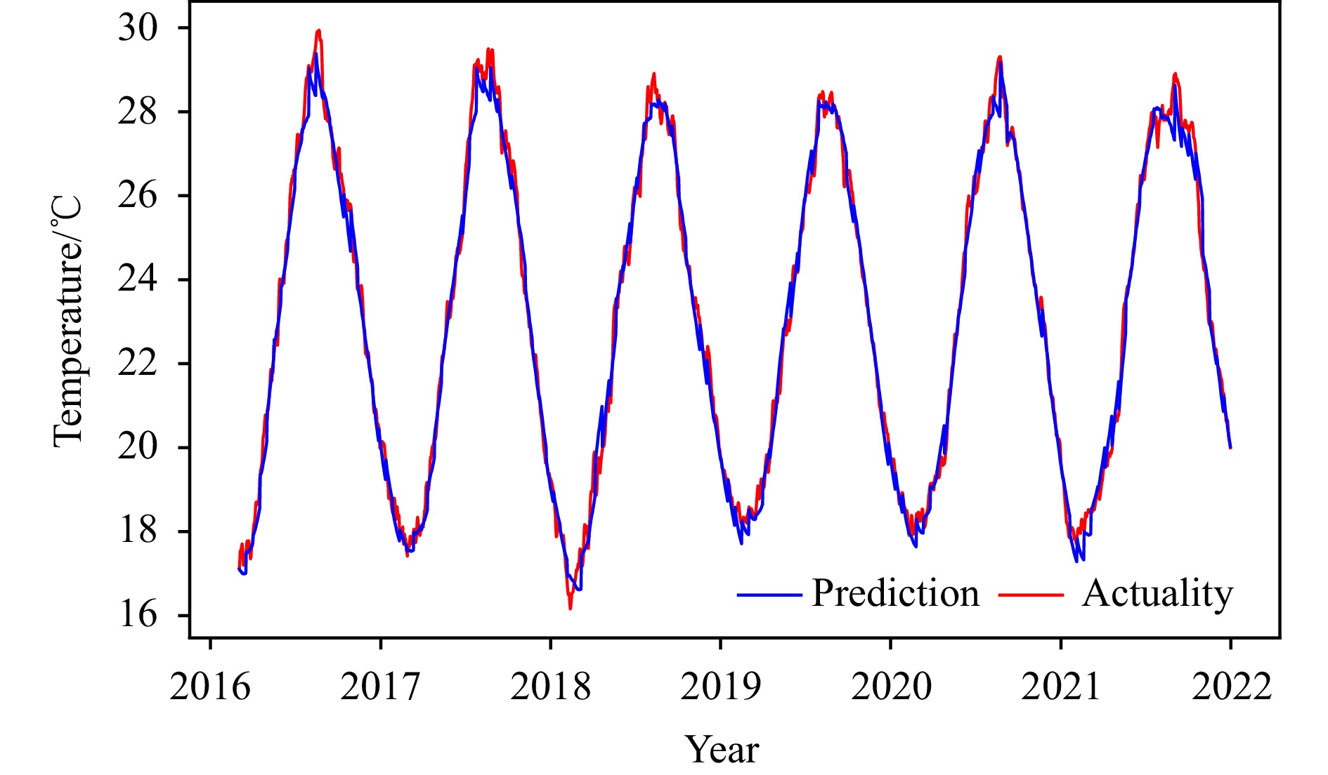
Using the continuous time-series dataset of OISST/SST from 2016 to 2021, we established "forecasting units" with a window size of 75 days (inputting 60 days and outputting 15 days) and slid this window along the dataset’s timestamp. The predictive results of the SST-MHW-DL model were aggregated to generate a continuous SST prediction sequence. In Fig. 8, the forecasted results closely align with the actual SST, exhibiting an error scale of less than 0.1℃. However, noticeable errors, nearing 0.5℃, persist at the extremes of annual SST values (both extremely high and low temperatures). This discrepancy primarily arises from the low percentage of these extreme data points within the overall dataset, resulting in insufficient model training. It is crucial to highlight that the predicted SST derived from SST-MHW-DL model demonstrates good consistency with observed SST values over long-term sequences, thereby providing robust support for using forecasted SST data in MHW detection.
 Figure 8. Forecast effectiveness evaluation of the SST-MHW-DL model.
4.2 Model Attention
To achieve robust forecasting results, previous studies commonly selected historical observational data inputs approximately four times the length of the forecasted duration (Zhang et al., 2017; Xiao et al., 2019). Consequently, the initial setup of the SST-MHW-DL model was configured with a 60-day length for the input historical SST data, constituting four times the expected forecast duration of 15 days. This study uses a channel attention module to explore the temporal relationships between the input historical data and the forecasted output results. Through a comprehensive forward propagation analysis of the trained model, we sequentially input historical SST data from the training, testing, and validation sets to calculate the time weight distribution for each dataset. By quantitatively analyzing the average contribution of data from different time periods to prediction accuracy, we identified the key time points that significantly influence the final prediction outcomes. This refined weight analysis provides deeper insights into the model’s temporal dependencies and decision-making mechanisms, allowing for the precise identification of the most critical time periods for accurate predictions. As shown in Fig. 9, the weight distributions of historical data in the past 60 days reveal that the SST information within the nearest 10 days to the forecast period holds the most significant data relevance to predict results (highlighted as the high-weight area in Fig. 9). However, previous days from 11 to 60 still retain a certain amount of temporal information (illustrated as the low-weight area in Fig. 9). Notably, Figure 9 indicates that the volume of information within historical data from days 11 to 60 does not linearly decrease with increasing time intervals. Hence, there is potential for further shortening the length of the input historical SST to reduce model complexity and computational resource consumption during the training process. Experimental findings revealed that historical SST data twice the forecast length already encompasses sufficient temporal information, exhibiting an RMSE of 0.639℃, which remains nearly unchanged in predictive accuracy compared to the fourfold length of 0.645℃. The temporal mechanisms revealed in our AI-based research do not conflict with existing physical mechanisms but have simply not been extensively explored before. AI models have already identified phenomena that traditional physical models have missed. For instance, Wang and Li (2024) were the first to determine, through interpretable machine learning methods, the crucial role of ocean salinity in ENSO predictions over timescales exceeding one year. In the future, AI will not only focus on aligning statistical results with physical mechanisms but also provide new perspectives and insights into the discovery and understanding of oceanic processes.
 Figure 9. Visualization of channel (temporal) attention weights in the SST-MHW-DL model.
Utilizing the spatial attention module, the SST-MHW-DL model obtained the weight distribution of the historical SST input in the spatial domain. Figure 10a shows that the deep-sea regions and the Taiwan Strait received more weight support, indicating their significant contribution to SST prediction. This observation aligns with prior studies, which have demonstrated that SST anomalies in the ECS are predominantly driven by the Kuroshio, the western boundary current of the North Pacific subtropical gyre, and its branch, the Taiwan Warm Current (Sasaki and Umeda, 2021). Furthermore, in the Kuroshio region, the upstream upwelling area (highlighted in green in Fig. 10a) contributes more to the overall temperature trend than downstream horizontal transport (Wei et al., 2023), as the Kuroshio’s overall trend is closely linked to changes in the upstream region. Our model successfully captures this critical upwelling area, assigning it the highest weight. Although coastal areas are also significant contributors to SST anomalies, the model assigns less focus to these regions, largely due to the lower accuracy of OISST data near the coast. Specifically, the RMSE of the SST-MHW-DL model for 15-day SST forecasts remains below 1℃, while the RMSE of OISST data in coastal regions occasionally exceeds 1℃ (Lee et al., 2021). Moreover, the spatial attention-derived weight heatmaps in Fig. 10 exhibited an extremely similar pattern to the temperature distribution in the East China Sea during spring and autumn. This suggests that the SST-MHW-DL model effectively captured the seasonal and geographical characteristics in the ECS region using the spatial attention mechanism. Studies have shown that SST in the ECS is significantly influenced by monsoon strength, shortwave radiation, and frontal activity during summer and winter (Tseng et al., 2000; Bao and Ren, 2014; Gao et al., 2020; Cao et al., 2021), resulting in greater SST fluctuations during these periods. By contrast, SST variations are more stable in spring and autumn, with a stronger correlation between historical and future SST. Consequently, the spatial attention mechanism places greater emphasis on these seasons to enhance prediction accuracy.
 Figure 10. Spatial attention in the SST-MHW-DL model. a. Weight distribution of the SST-MHW-DL model. b. Spring temperature. c. Autumn temperature.
In practical applications, near-real-time SST data from remote sensing can be applied to the SST-MHW-DL model proposed in the paper, but with certain limitations. While datasets such as AVHRR, MODIS, VIIRS, and Sentinel-3 SLSTR offer high spatial and temporal resolutions, they are often incomplete due to factors like cloud cover and require significant post-processing to correct for atmospheric effects. The higher error rates in near-real-time data can lead to the rapid accumulation of forecast errors, potentially shortening the effective forecast period. For instance, predictions that could extend up to 15 days with post-processed data may be reduced to around 7 days with near-real-time data. Although near-real-time data offers more frequent updates, it may not be as reliable as post-processed datasets like OISST, which undergo rigorous corrections to ensure greater accuracy and continuity, making them better suited for long-term forecasts. Thus, while near-real-time SST data can be used, its application may require adjustments to account for the increased error and shorter forecast horizons.
4.3 Detecting MHW
Employing the forecast values and actual observed OISST/SST values from 2016 to 2021, the MHW events are detected in each pixel in the ECS region. These predicted MHW events were compared against corresponding actual (labeled) data for MHW events, as shown in Table 2. The total number of SST grid points that experienced MHW but were not forecasted amounted to
811248 (FN), while those that neither experienced MHW nor were forecasted totaled2837509 (TN) grid points. Grid points where MHW occurred and were forecasted accounted for614912 (TP), and grid points where MHW events did not happen but were forecasted amounted to224133 (FP). We computed three evaluation metrics for the SST-MHW-DL model, achieving an accuracy of 0.77, precision of 0.73, and recall of 0.43. These metrics indicate that the proposed SST-MHW-DL model can effectively forecast marine heatwave events.Table 2. Diffusion matrix for MHW detection in the ECSMHWs predicted MHWs not predicted MHWs observed 614912 (TP)811248 (FN)MHWs not
observed224133 (FP)2837509 (TN)| Show TableDownLoad:
CSV
To thoroughly assess the forecasting performance of the SST-MHW-DL model concerning heatwave outbreaks across the ECS, we analyzed three distinct periods of MHW events, each representing varying scales of coverage. These events comprised instances with coverage proportions of 25% (occurring between January 5, 2021, and March 19, 2021), 50% (from March 5, 2019, to March 19, 2019), and 75% (spanning October 15, 2016, to October 29, 2016). As shown in Fig. 11, during these periods, the proportion of accurately predicted areas (TN+TP) in the total area surpassed 99%, highlighting the high predictive capability of the SST-MHW-DL model. This underscores the model’s effectiveness in forecasting heatwave outbreaks across diverse scales, with the majority of regions exhibiting commendable accuracy and consistency in the forecasted results.
 Figure 11. Detection of MHW with different occurrence scales of 25%, 50%, and 75% in the ECS. TP and TN denote correctly predicted MHW sea areas.
Additionally, a statistical analysis was conducted on all historical MHW events from 2016 to 2021 to explore the spatiotemporal characteristics of MHW occurrence across the ECS region. Figure 12 illustrates that the annual average MHW intensity remained below 1℃ (Fig. 12a), falling below the average intensity range of global MHWs (Marin et al., 2021). The average duration of MHWs was 16.7 days (Fig. 12b). However, in critical areas such as the Taiwan Strait, Kuroshio path, and the mouth of the Changjiang River, the frequency of MHWs reached as high as 9 times per year (Fig. 12c), significantly surpassing the global average frequency (1−3 times/year) (Holbrook et al., 2019).
 Figure 12. Spatiotemporal statistics of MHW occurrence in the ECS from 2016 to 2021. a. Average intensity (℃). b. Occurrence duration of the MHW events (days). c. Annual average occurrence frequency (counts/year).
4.4 Temporal mechanism and model validation
The Northwest Atlantic (NWA), particularly the continental shelf off the northeastern United States (35°N−52°N, 77°W−51°W), ranks among the fastest-warming regions globally (Pershing et al., 2018; Chen et al., 2020). As shown in Fig. 13, certain areas within this region have depths of only a few tens of meters, with most areas not exceeding 5,000 meters. The trend in the monthly average SST is significant, with most areas experiencing changes greater than 1℃. This warming trend increases the risk of MHW and imposes cumulative thermal stress on marine ecosystems. We selected this region for testing to validate the proposed SST-MHW-DL model and the discovered temporal mechanisms, using historical SST data from the past 30 days (twice the predicted length) to predict SST changes and MHW occurrences over the next 15 days. The model was trained and validated using data from 1981-2015 and tested with data from 2016-2021.
 Figure 13. Test area. a. Topography of the NWA. b. SST variations in the NWA from 2016 to 2021.
To better understand the spatiotemporal characteristics of MHWs in this region, we statistically analyzed their occurrences from 2016 to 2021. As shown in Fig. 14, the average intensity and duration of MHWs were 0.75℃ and 21.6 days, respectively (Figs 13a and b), significantly higher than those in the ECS. This elevated intensity and duration increase the difficulty of SST prediction and MHW detection. MHWs occurred throughout the region, with local frequencies exceeding 10 events per year (Fig. 14c).
 Figure 14. Spatiotemporal statistics of MHW occurrence in the NWA from 2016 to 2021. a. Average intensity (℃). b. Occurrence duration of the MHW events (days). c. Annual average occurrence frequency (counts/year).
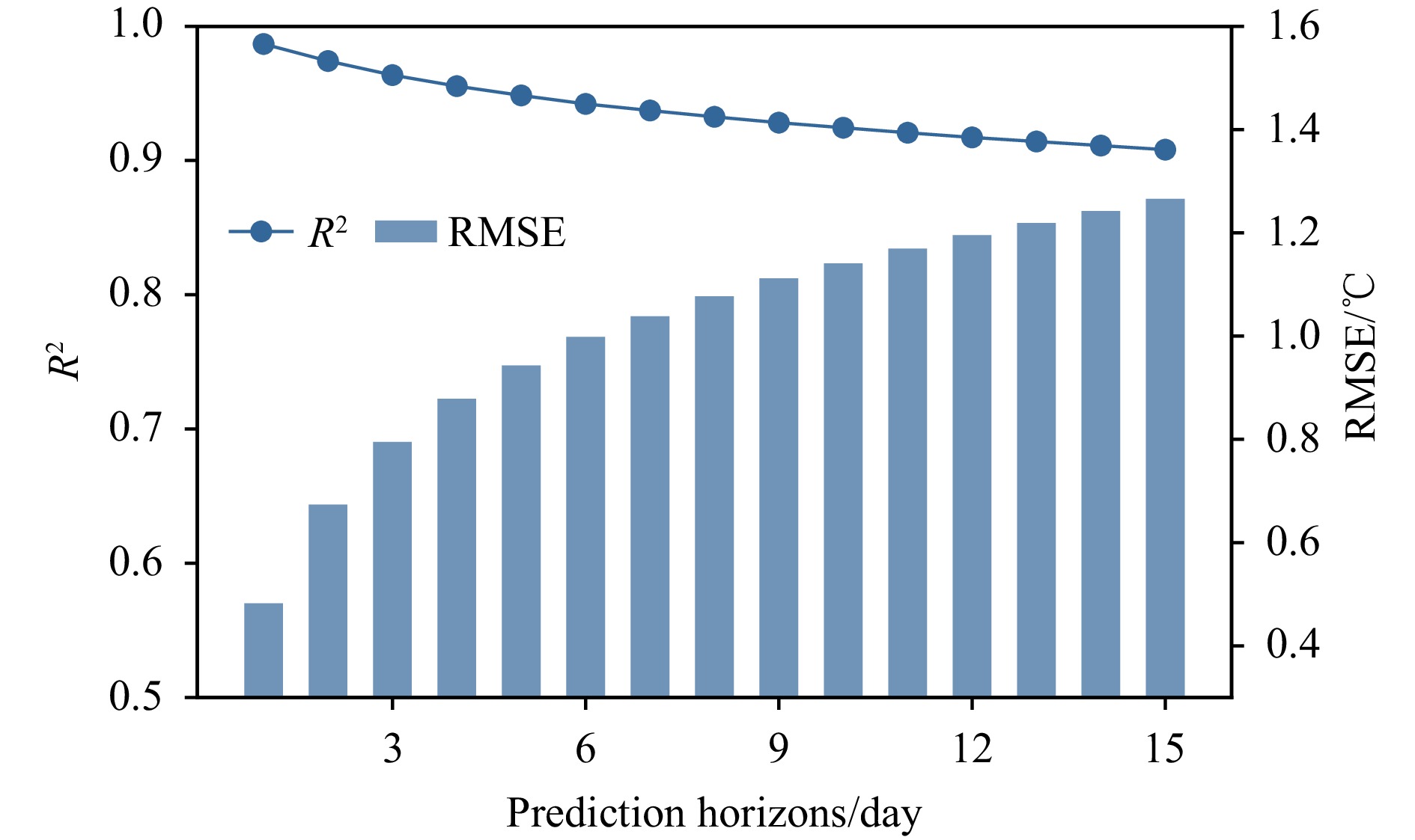
As shown in Fig. 15, during the SST forecasting phase, the model’s RMSE increased to 1℃ compared to the ECS region, due to the higher variability of SST in this area. Notably, the R² value in this region showed a significant improvement over the ECS, remaining around 0.9 by the 15th day of prediction, demonstrating the model’s high responsiveness to SST data. Additionally, it is important to note that to better demonstrate the proposed model’s applicability, the model’s layers and the number of neurons per layer were not adjusted despite the increased size of the study area.
 Figure 15. RMSE and R² of SST forecast.
Figure 16 illustrates the spatial distribution of RMSE (Fig. 16a) and R² (Fig. 16b) between predicted and observed SST in the NWA, along with an evaluation of prediction effectiveness (Fig. 16c). Our SST prediction model demonstrates notably low RMSE and high R² across most observational data, indicating high accuracy and strong correlation. In the central eastern part of the Northwest Atlantic, RMSE is relatively high (approximately 2℃), while R² is relatively low (around 0.8), suggesting some challenges in prediction accuracy in this region. Fig. 16c highlights the strong consistency between our predicted SST and long-term observed values, especially during periods of extreme annual average temperatures, with minimal discrepancies. These findings further validate the reliability of the SST-MHW-DL model in accurately forecasting SST in the NWA.
 Figure 16. Spatial distribution of (a) RMSE (℃) and (b) R2 predicted by SST, as well as (c) the effectiveness evaluation of the model’s predictions.
Using the SST values predicted by the model, MHW events were detected in each pixel of the NWA. As shown in Table 3, the total number of SST grid points that experienced MHW but were not predicted (FN) is
1284398 , while the total number of SST grid points that neither experienced nor were predicted to experience MHW (TN) is811248 . The number of grid points where MHW events were both observed and predicted (TP) is2063321 , and the number of grid points where MHW events were predicted but not observed (FP) is589214 . We calculated three evaluation metrics for the SST-MHW-DL model in this region: accuracy, precision, and recall, which are 0.79, 0.78, and 0.62, respectively. These metrics indicate that the proposed SST-MHW-DL model and temporal mechanism are effective in predicting MHW events in the NWA.Table 3. Diffusion matrix for MHW detection in the NWAMHWs predicted MHWs not predicted MHWs observed 2063321 (TP)1284398 (FN)MHWs not observed 589214 (FP)811248 (TN)| Show TableDownLoad:
CSV
5. Conclusion
This study introduces the SST-MHW-DL model to address the challenge of predicting relatively rare heatwave events with short-term forecasts of two weeks. The SST-MHW-DL model leverages the ConvLSTM architecture and an attention mechanism to address two key processes: SST prediction and MHW detection. Utilizing past 60-day SST data, the model forecasts SST and associated MHW occurrences for the subsequent 15 days. Trained on data from the ECS from 1980 to 2015 and tested on data from 2016 to 2021, the model demonstrates notable accuracy in both SST prediction and heatwave detection.
The primary findings of this study are as follows: (1) The SST-MHW-DL model achieves an RMSE of 0.64℃, a MAPE of 2.05%, and an R² of 0.85, indicating high accuracy in predicting sea surface temperatures in the ECS region. For SST-based heatwave detection, the model achieves an accuracy of 0.77, precision of 0.73, and recall of 0.43, demonstrating its capability in effectively identifying MHW events. (2) The study employs an attention mechanism to examine the influence of historical data on forecasted outputs. The “channel attention” mechanism reveals that SST data from the closest 10 days to the prediction period significantly impacts the forecast results more than earlier periods. Contrary to previous assumptions suggesting a four-fold input data duration, the mechanism suggests that historical data only needs to be twice the forecast duration to encompass the most relevant information, maintaining consistent predictive accuracy. Additionally, the "spatial attention" mechanism analyzes the contribution of different regions in the East China Sea to SST prediction. It finds that deep-sea areas closer to the northwestern Pacific contribute more significantly due to their stable SST structure, while coastal areas experience more dramatic SST variations influenced by nearshore currents and freshwater input. (3) This study validates the proposed SST-MHW-DL model and the identified temporal mechanism in the marine heatwave-prone NWA region, achieving promising results. The model’s performance in SST forecasting achieved an RMSE of 1.02℃ and an R² of 0.94. For heatwave detection, the accuracy, precision, and recall were 0.79, 0.78, and 0.62, respectively, demonstrating the model’s robust performance in different regions. Future improvements may involve integrating hydrological and meteorological data into the SST-MHW-DL model, potentially enhancing forecasting performance further.
-
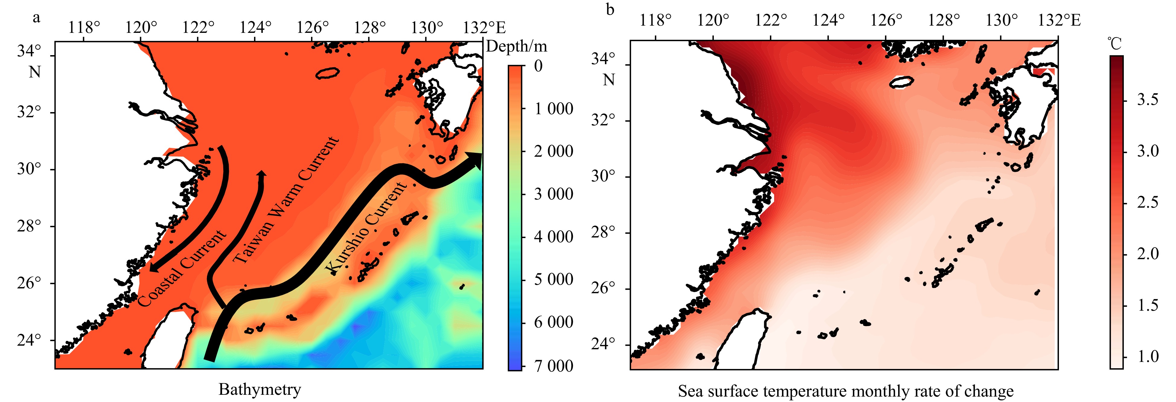
Figure 1. Study area. (a) Topography of the ECS and its primary ocean currents, (b) SST variations in the ECS from 2016 to 2021.

Figure 3. Structural diagram of the proposed SST-MHW-DL model (the red box highlights our improvement and analysis part).
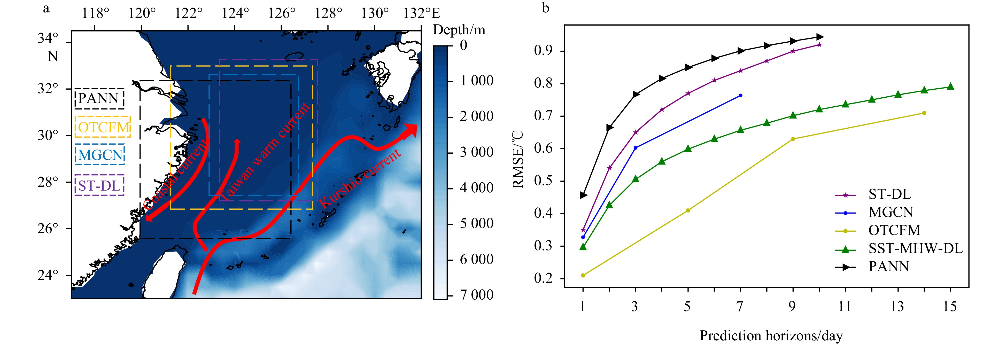
Figure 6. Comparison between the SST-MHW-DL model and several state-of-the-art models. a. Comparison of study areas. b. Accuracy comparison for different forecast durations.

Figure 7. Spatiotemporal variations in SST forecast errors by the SST-MHW-DL model in the ECS region. a. Difference RMSE of the predicted SST and ground truth. b. RMSE of the predicted SST and ground truth.
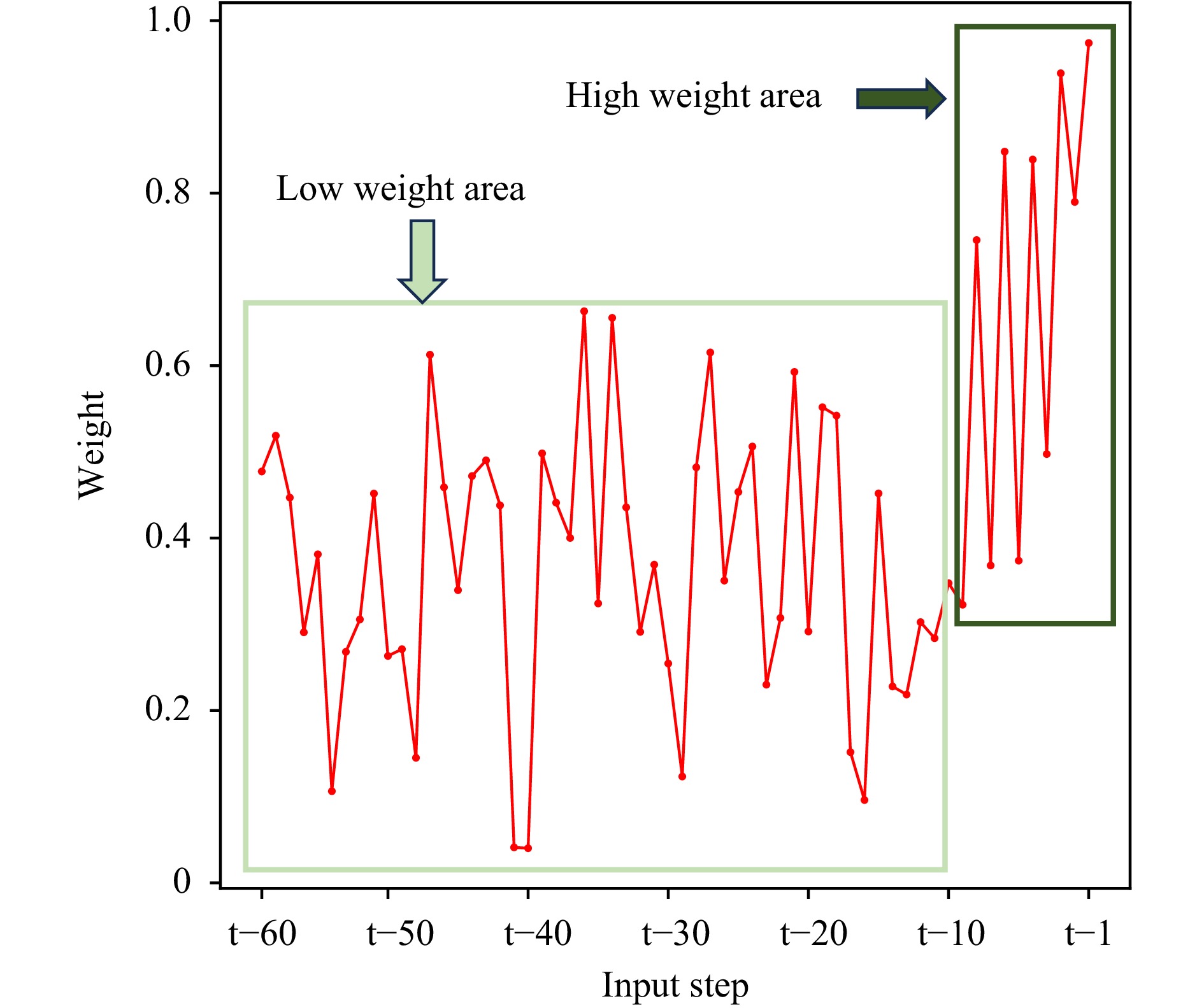
Figure 9. Visualization of channel (temporal) attention weights in the SST-MHW-DL model.
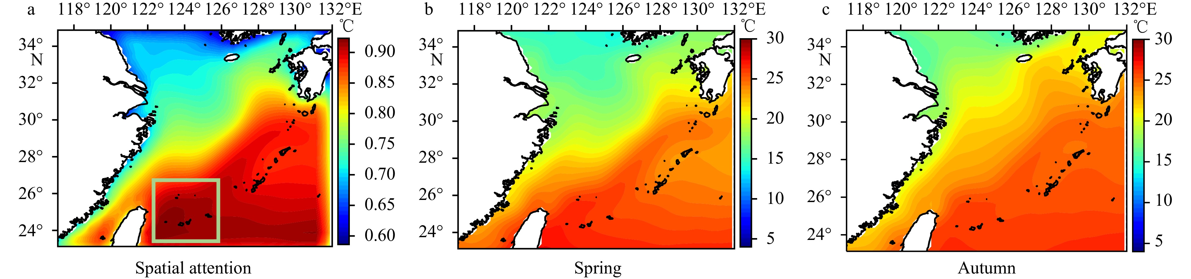
Figure 10. Spatial attention in the SST-MHW-DL model. a. Weight distribution of the SST-MHW-DL model. b. Spring temperature. c. Autumn temperature.
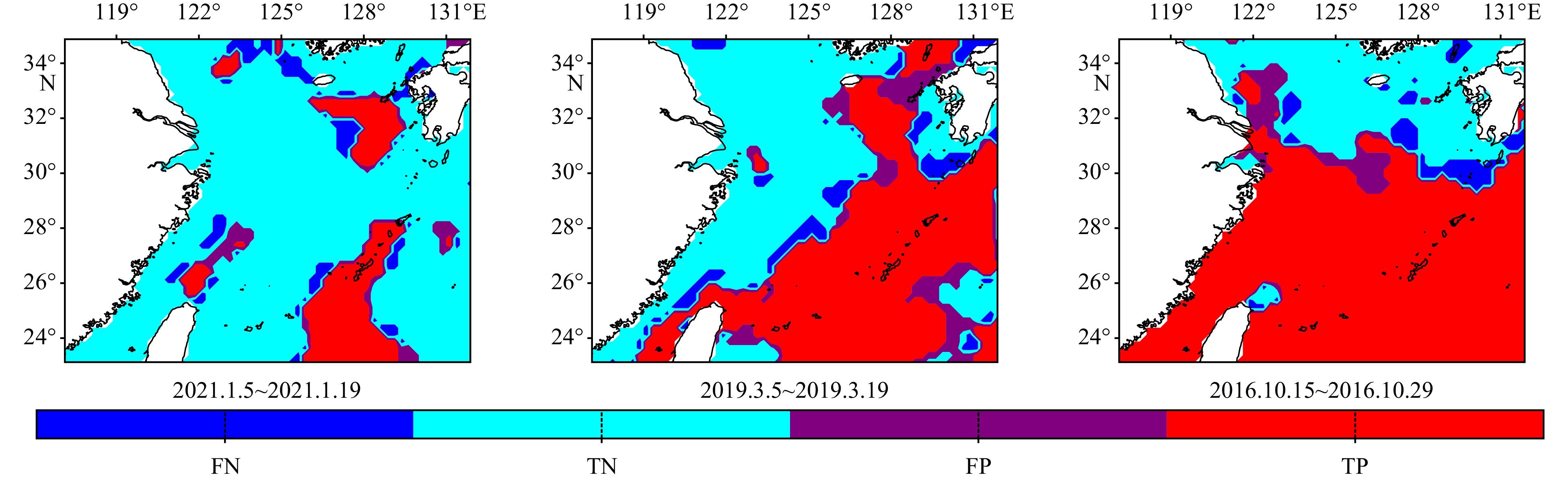
Figure 11. Detection of MHW with different occurrence scales of 25%, 50%, and 75% in the ECS. TP and TN denote correctly predicted MHW sea areas.

Figure 12. Spatiotemporal statistics of MHW occurrence in the ECS from 2016 to 2021. a. Average intensity (℃). b. Occurrence duration of the MHW events (days). c. Annual average occurrence frequency (counts/year).
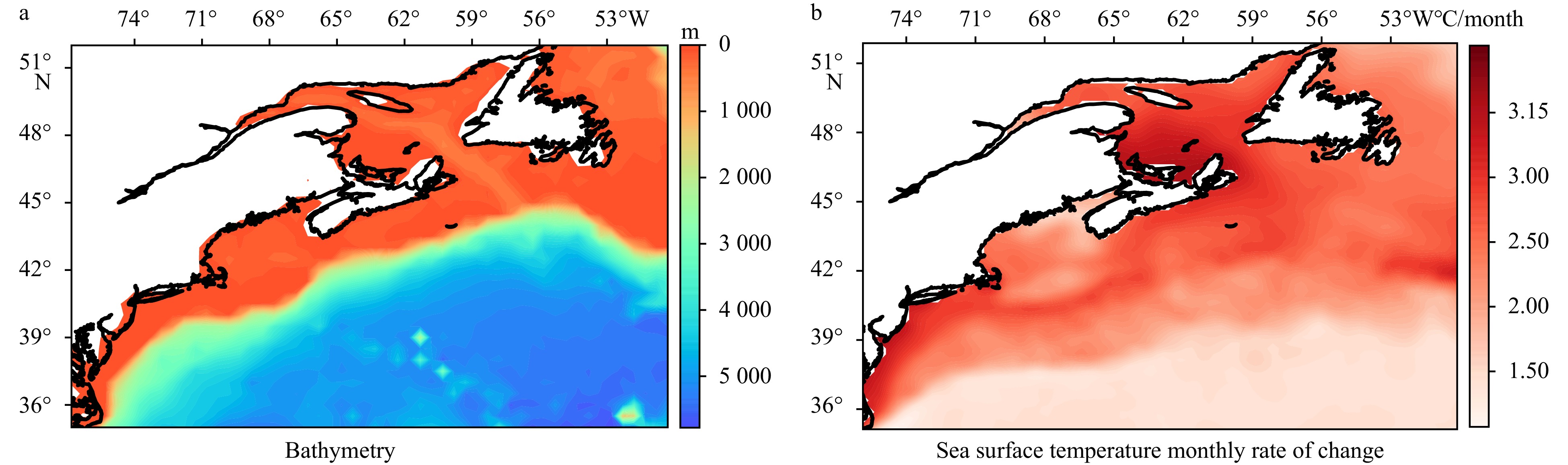
Figure 13. Test area. a. Topography of the NWA. b. SST variations in the NWA from 2016 to 2021.
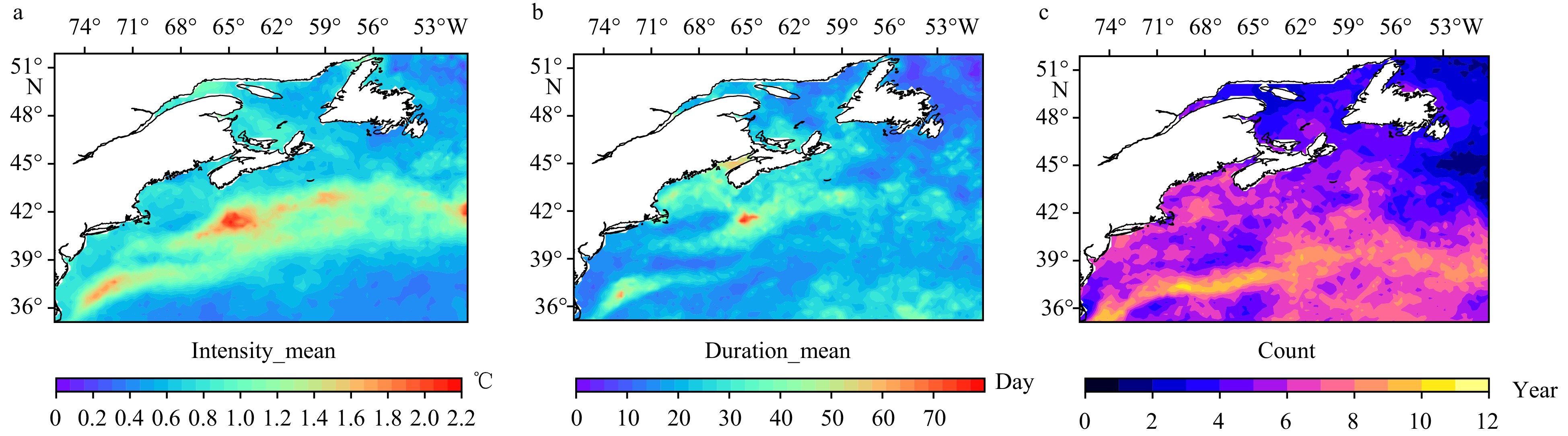
Figure 14. Spatiotemporal statistics of MHW occurrence in the NWA from 2016 to 2021. a. Average intensity (℃). b. Occurrence duration of the MHW events (days). c. Annual average occurrence frequency (counts/year).

Figure 16. Spatial distribution of (a) RMSE (℃) and (b) R2 predicted by SST, as well as (c) the effectiveness evaluation of the model’s predictions.
Table 1. Comparison of the proposed SST-MHW-DL with basic ConvLSTM, U-Net, and Multi-attention ConvLSTM models
Model RMSE/℃ MAPE/% R2 ConvLSTM 0.67 2.13 0.846 U-Net 0.73 2.35 0.823 Multi-Attention ConvLSTM 0.66 2.14 0.850 SST-MHW-DL 0.64 2.05 0.854  下载: 导出CSV
Table 2. Diffusion matrix for MHW detection in the ECS
MHWs predicted MHWs not predicted MHWs observed 614912 (TP)811248 (FN)MHWs not
observed224133 (FP)2837509 (TN)
下载: 导出CSV
Table 3. Diffusion matrix for MHW detection in the NWA
MHWs predicted MHWs not predicted MHWs observed 2063321 (TP)1284398 (FN)MHWs not observed 589214 (FP)811248 (TN)
下载: 导出CSV
-
Bao Baoleerqimuge, Ren Guoyu. 2014. Climatological characteristics and long-term change of SST over the marginal seas of China. Continental Shelf Research, 77: 96–106, doi: 10.1016/j.csr.2014.01.013 Bian Ce, Jing Zhao, Wang Hong, et al. 2023. Oceanic mesoscale eddies as crucial drivers of global marine heatwaves. Nature Communications, 14(1): 2970, doi: 10.1038/s41467-023-38811-z Cao Lu, Tang Rui, Huang Wei, et al. 2021. Seasonal variability and dynamics of coastal sea surface temperature fronts in the East China Sea. Ocean Dynamics, 71(2): 237–249, doi: 10.1007/s10236-020-01427-8 Cao Lu, Tang Rui, Huang Wei, et al. 2021. Seasonal variability and dynamics of coastal sea surface temperature fronts in the East China Sea. Ocean Dynamics, 71(2): 237–249, doi: 10.1007/s10236-020-01427-8 Chen Zhuomin, Kwon Y O, Chen Ke, et al. 2020. Long-term SST variability on the Northwest Atlantic continental shelf and slope. Geophysical Research Letters, 47(1): e2019GL085455, doi: 10.1029/2019GL085455 Claar D C, Wood C L. 2020. Pulse heat stress and parasitism in a warming world. Trends in Ecology & Evolution, 35(8): 704–715, doi: 10.1016/j.tree.2020.04.002 De Burgh-Day C O, Spillman C M, Smith G, et al. 2022. Forecasting extreme marine heat events in key aquaculture regions around New Zealand. Journal of Southern Hemisphere Earth Systems Science, 72(1): 58–72, doi: 10.1071/es21012 Fan Luyi, Cao Yuhao, Huang Ningyuan, et al. 2024. OTCFM: a sea surface temperature prediction method integrating multi-scale periodic features. IEEE Access, 12: 108291–108302, doi: 10.1109/ACCESS.2024.3425514 Fredston A L, Cheung W W L, Frölicher T L, et al. 2023. Marine heatwaves are not a dominant driver of change in demersal fishes. Nature, 621(7978): 324–329, doi: 10.1038/s41586-023-06449-y Frölicher T L, Fischer E M, Gruber N. 2018. Marine heatwaves under global warming. Nature, 560(7718): 360–364, doi: 10.1038/s41586-018-0383-9 Gao Guandong, Marin M, Feng Ming, et al. 2020. Drivers of marine heatwaves in the East China Sea and the South Yellow Sea in three consecutive summers during 2016–2018. Journal of Geophysical Research: Oceans, 125(8): e2020JC016518, doi: 10.1029/2020JC016518 Giamalaki K, Beaulieu C, Prochaska J X. 2022. Assessing predictability of marine heatwaves with random forests. Geophysical Research Letters, 49(23): e2022GL099069, doi: 10.1029/2022gl099069 Han Mingxu, Feng Yuan, Zhao Xueli, et al. 2019. A convolutional neural network using surface data to predict subsurface temperatures in the Pacific Ocean. IEEE Access, 7: 172816–172829, doi: 10.1109/ACCESS.2019.2955957 Hobday A J, Alexander L V, Perkins S E, et al. 2016. A hierarchical approach to defining marine heatwaves. Progress in Oceanography, 141: 227–238, doi: 10.1016/j.pocean.2015.12.014 Hobday A J, Spillman C M, Eveson J P, et al. 2018. A framework for combining seasonal forecasts and climate projections to aid risk management for fisheries and aquaculture. Frontiers in Marine Science, 5: 137, doi: 10.3389/fmars.2018.00137 Holbrook N J, Scannell H A, Sen Gupta A, et al. 2019. A global assessment of marine heatwaves and their drivers. Nature Communications, 10(1): 2624, doi: 10.1038/s41467-019-10206-z Hövel L, Brune S, Baehr J. 2022. Decadal prediction of marine heatwaves in MPI-ESM. Geophysical Research Letters, 49(15): e2022GL099347, doi: 10.1029/2022GL099347 Hu Shijian, Li Shihan. 2022. Progress and prospect of marine heatwave study. Advances in Earth Science (in Chinese), 37(1): 51–64, doi: 10.11867/j.issn.10018166.2021.121 Iskandar M R, Ismail M F A, Arifin T, et al. 2021. Marine heatwaves of sea surface temperature off south Java. Heliyon, 7(12): e08618, doi: 10.1016/j.heliyon.2021.e08618 Jahanbakht M, Xiang Wei, Azghadi M R. 2022. Sea surface temperature forecasting with ensemble of stacked deep neural networks. IEEE Geoscience and Remote Sensing Letters, 19: 1502605, doi: 10.1109/lgrs.2021.3098425 Kako S, Nakagawa T, Takayama K, et al. 2016. Impact of Changjiang River discharge on sea surface temperature in the East China Sea. Journal of Physical Oceanography, 46(6): 1735–1750, doi: 10.1175/jpo-d-15-0167.1 Lee M A, Huang W P, Shen Y L, et al. 2021. Long-term observations of interannual and decadal variation of sea surface temperature in the Taiwan Strait. Journal of Marine Science and Technology, 29(4): 7, doi: 10.51400/2709-6998.1587 Lee E Y, Park K A. 2021. Validation satellite sea surface temperature in the coastal regions. In: Proceedings of 2021 IEEE International Geoscience and Remote Sensing Symposium IGARSS. Brussels, Belgium: IEEE,7607–7610, doi: 10.1109/IGARSS47720.2021.9553695 Lian Peng, Gao Le. 2024. Impacts of central-Pacific El Niño and physical drivers on eastern Pacific bigeye tuna. Journal of Oceanology and Limnology, 42(3): 972–987, doi: 10.1007/s00343-023-3051-3 Marin M, Feng Ming, Phillips H E, et al. 2021. A global, multiproduct analysis of coastal marine heatwaves: Distribution, characteristics, and long-term trends. Journal of Geophysical Research: Oceans, 126(2): e2020JC016708, doi: 10.1029/2020JC016708 Oliver E C J, Benthuysen J A, Darmaraki S, et al. 2021. Marine heatwaves. Annual Review of Marine Science, 13: 313–342, doi: 10.1146/annurev-marine-032720-095144 Oliver E C J, Donat M G, Burrows M T, et al. 2018. Longer and more frequent marine heatwaves over the past century. Nature Communications, 9(1): 1324, doi: 10.1038/s41467-018-03732-9 Pearce A, Lenanton R, Jackson G, et al. 2011. The “marine heat wave” off Western Australia during the summer of 2010/11. Fisheries Research Report No. 222, Western: Department of Fisheries, 40 Pershing A J, Mills K E, Dayton A M, et al. 2018. Evidence for adaptation from the 2016 marine heatwave in the northwest Atlantic Ocean. Oceanography, 31(2): 152–161, doi: 10.5670/oceanog.2018.213 Ren Yibin, Li Xiaofeng. 2023. Predicting the daily sea ice concentration on a subseasonal scale of the Pan-Arctic during the melting season by a deep learning model. IEEE Transactions on Geoscience and Remote Sensing, 61: 4301315, doi: 10.1109/TGRS.2023.3279089 Sasaki Y N, Umeda C. 2021. Rapid warming of sea surface temperature along the Kuroshio and the China coast in the East China Sea during the twentieth century. Journal of Climate, 34(12): 4803–4815, doi: 10.1175/JCLI-D-20-0421.1 Shanks A L, Rasmuson L K, Valley J R, et al. 2020. Marine heat waves, climate change, and failed spawning by coastal invertebrates. Limnology and Oceanography, 65(3): 627–636, doi: 10.1002/lno.11331 Shi Xingjian, Chen Zhourong, Wang Hao, et al. 2015. Convolutional LSTM network: a machine learning approach for precipitation nowcasting. arXiv: 1506.04214, 2015 Shi Benyun, Feng Liu, He Hailun, et al. 2024. A physics-guided attention-based neural network for sea surface temperature prediction. IEEE Transactions on Geoscience and Remote Sensing, 62: 4210413, doi: 10.1109/TGRS.2024.3457039 Smith K E, Burrows M T, Hobday A J, et al. 2021. Socioeconomic impacts of marine heatwaves: global issues and opportunities. Science, 374(6566): eabj3593, doi: 10.1126/science.abj3593 Smith K E, Burrows M T, Hobday A J, et al. 2023. Biological impacts of marine heatwaves. Annual Review of Marine Science, 15: 119–145, doi: 10.1146/annurev-marine-032122-121437 Tseng C, Lin Chiyuan, Chen Shihchin, et al. 2000. Temporal and spatial variations of sea surface temperature in the East China Sea. Continental Shelf Research, 20(4–5): 373–387, doi: 10.1016/S0278-4343(99)00077-1 Wang Haoyu, Hu Shineng, Guan Cong, et al. 2024. The role of sea surface salinity in ENSO forecasting in the 21st century. npj Climate and Atmospheric Science, 7(1): 206, doi: 10.1038/s41612-024-00763-6 Wang Haoyu, Li Xiaofeng. 2024. DeepBlue: advanced convolutional neural network applications for ocean remote sensing. IEEE Geoscience and Remote Sensing Magazine, 12(1): 138–161, doi: 10.1109/mgrs.2023.3343623 Wang Fan, Li Xuegang, Tang Xiaohui, et al. 2023a. The seas around China in a warming climate. Nature Reviews Earth & Environment, 4(8): 535–551, doi: 10.1038/s43017-023-00453-6 Wang Yunhe, Yuan Xiaojun, Ren Yibin, et al. 2023b. Subseasonal prediction of regional antarctic sea ice by a deep learning model. Geophysical Research Letters, 50(17): e2023GL104347, doi: 10.1029/2023gl104347 Wang Zihan, Zeng Cong, Cao Ling. 2023c. Mapping the biodiversity conservation gaps in the East China sea. Journal of Environmental Management, 336: 117667, doi: 10.1016/j.jenvman.2023.117667 Wei Yi, Ding Ruibin, Huang Daji, et al. 2023. The weakened upwelling at the Upstream Kuroshio in the East China Sea induced extensive sea surface warming. Geophysical Research Letters, 50(1): e2022GL101835, doi: 10.1029/2022gl101835 Woo S, Park J, Lee J Y, et al. 2018. CBAM: convolutional block attention module. In Proceedings of the 15th European Conference on Computer Vision. Munich, Germany: Springer,3–19 Xiao Changjiang, Chen Nengcheng, Hu Chuli, et al. 2019. A spatiotemporal deep learning model for sea surface temperature field prediction using time-series satellite data. Environmental Modelling & Software, 120: 104502, doi: 10.1016/j.envsoft.2019.104502 Yu Haiqing, Wang Hui, Yuan Chunxin, et al. 2024. Assessing the predictability of the marine heatwave in the Yellow Sea during the summer of 2018 based on a deterministic forecast model. Weather and Climate Extremes, 44: 100663, doi: 10.1016/j.wace.2024.100663 Zhang Kun, Geng Xupu, Yan Xiaohai. 2020. Prediction of 3-D ocean temperature by multilayer convolutional LSTM. IEEE Geoscience and Remote Sensing Letters, 17(8): 1303–1307, doi: 10.1109/LGRS.2019.2947170 Zhang Xiaoyu, Li Yongqing, Frery A C, et al. 2022. Sea surface temperature prediction with memory graph convolutional networks. IEEE Geoscience and Remote Sensing Letters, 19: 8017105, doi: 10.1109/lgrs.2021.3097329 Zhang Qin, Wang Hui, Dong Junyu, et al. 2017. Prediction of sea surface temperature using Long Short-Term Memory. IEEE Geoscience and Remote Sensing Letters, 14(10): 1745–1749, doi: 10.1109/LGRS.2017.2733548 -

 DownLoad:


 点击查看大图
计量
- 文章访问数: 41
- HTML全文浏览量: 15
- 被引次数: 0

