

Field observation of air-sea CO2 and H2O flux using the eddy covariance method based on 100 Hz gas analyzer in the Bohai and Yellow Seas
-
Abstract: Air-sea water vapor and CO2 flux observation experiments were carried out at the Yantai National Satellite Ocean Calibration Platform and the jetty at Monolithic Beach, Juehua Island, using a 100 Hz gas analyzer. The observations were corrected by employing wild point rejection, linear detrending, delay correction, coordinate rotation, time matching, and WPL correction. The results of spectral analysis and a turbulence development adequacy data quality check showed that the overall observation data quality was good. The air-sea water vapor and CO2 flux results showed that the observation duration affected both the air-sea flux intensity and direction at different observation frequencies. At shorter observation durations, the air-sea flux values measured at 100 Hz were smaller than the 20 Hz measurements and had opposite directions. In addition, the WPL correction reduced the overall air-sea flux and partially minimized the effect of observation frequency on the air-sea flux intensity. These results showed that high-frequency observations showed more turbulence variations than low-frequency observations. This conclusion could promote an understanding of small-scale turbulence variations.
-
Key words:
- Eddy correlation method /
- 100 Hz /
- Gas analyzer /
- TDLAS /
- Air-sea flux /
- Observation frequency
-
1. Introduction
CO2 is the most important anthropogenic greenhouse gas, and its increasing concentration is accelerating climate change (Liu et al., 2022; IPCC, 2023). Furthermore, water vapor is also an important greenhouse gas (GHG), and changes in its tropospheric concentration affect climate while influencing the concentration of other GHGs in the atmosphere (Wuebbles et al., 1989; Coe et al., 2021). Accurate estimates of air-sea CO2 and water vapor fluxes are crucial to accurately predict and respond to climate change (Hart, 2006; Brevik, 2012; Kaye and Quemada, 2017; Shukla et al., 2019).
In situ observation, using either a box method or a micrometeorological method, is an important method for studying air-sea flux (Hu et al., 2014). For different downwelling environmental conditions and the needs of long-term and continuous in situ observation, the micrometeorological method (based on the principles of atmospheric thermodynamics and dynamics) is the best choice for air-sea flux observation (Siebicke and Emad, 2019). Micrometeorological methods include eddy covariance (EC) methods, mass balance methods, and vorticity accumulation methods (Baldocchi, 2003; Baldocchi et al., 1988; Mammarella et al., 2009; Palatella et al., 2014; Weber, 1999). The EC, which is a direct air-sea flux measurement technique with the advantages of requiring no empirical parameters and being easy to use for in situ observation, has undergone substantial development in recent decades (Horst, 2000; Eugster et al., 2000; Baldocchi, 2003; Shahan et al., 2022).
The eddy correlation method was originally proposed by Swinbank (1951) for the measurement of land-air heat, mass, and momentum changes. With the development of equipment (anemometers, computer storage media) and theory (hydrodynamics, micrometeorology), the method became more widely used (Matthews and Schume, 2022; Shahan et al., 2022; Czubaszek and Wysocka-Czubaszek, 2023; Rytwo and Eliyahou, 2023; Stagakis et al., 2023). As wobble platform calibration methods continue to be refined, there has been an increase in the number of studies focusing on air-sea flux observations carried out on instrumented platforms such as ships, buoys, and offshore platforms (Horst, 2000; Kondo and Tsukamoto, 2007; Miller et al., 2008, 2010; Else et al., 2011; Blomquist et al., 2012).
The rest of this paper is organized as follows. The study area and data, including the experimental platform and instrumentation setup are described in Section 2; the basic principles of the EC, quality control, and quality assessment methods are presented in Section 3; the results of the calibration, quality assessment, and air-sea flux calculations of the high-frequency and low-frequency data are analyzed and discussed in Section 4; finally, conclusions and perspectives are presented in Section 5.
2. Field observation experiment
2.1 Field observation platform
In this study, air-sea CO2 and water vapor flux observation experiments were carried out at the Yantai National Satellite Ocean Calibration Platform (hereafter referred to as the offshore platform) and the Sea Island Observation Platform (hereafter referred to as the sea island) at the Juehua Island Monolithic Beach Pier (Fig. 1). The offshore platform is 20 km away from land, which is conducive to the use of the eddy correlation method for air-sea interface flux observation. The island observation site is between the ocean and the land, which is conducive to understanding offshore air-sea exchange.
 Figure 1. Air-sea flux observation platforms. Symbol‘★’is the observation platform of Juehua Island, and‘▲’is the Yantai National Satellite Ocean Calibration Platform.
In current research on air-sea flux, few scholars have obtained such extensive field observation data for analysis. Many studies often choose to use near-shore meteorological observation stations or coastal scanning LiDAR (sLiDAR) for flux measurements, but both of our two observation platforms are island-based, allowing for direct measurements using instruments. By using a large number of direct sea observation data for subsequent air-sea flux calculations and comparative analysis between high and low frequency instruments, the results promise more accuracy, reliability, and significance for reference.
2.2 Experimental instruments and set-up
The offshore platform was fitted with a LI-
7500 H2O/ CO2 gas analyzer in combination with a Gill Ultrasonic Anemometer HS-100 for air-sea flux observations. Following the installation manual, the LI-7500 was tilted 10–15° during installation to avoid the obstruction of the mirror by water droplets. The 100 Hz CO2 pulsometer (Fig. 2a) and the water vapor pulsometer (Fig. 2b) were developed by the Hefei Institute of Physical Sciences of the Chinese Academy of Sciences, which adopted the TDLAS technology, high-frequency laser modulation technology, high-frequency signal acquisition, and processing technology. An inverse spectral concentration inversion method was used (Li et al., 2021b). The field installation of the high-frequency pulsometer is shown in Fig. 3. The installation needs to avoid shading the ultrasonic anemometer as much as possible to minimize the impact on the wind field. Figure 2. High-frequency 100 Hz pulsating gas analyzer. (a) CO2 gas analyzer; (b) H2O gas analyzer.
 Figure 3. In situ observation experiments. (a) and (b) are the Yantai National Satellite Ocean Calibration Platform and the island observation platform at Juehua Island, Liaoning Province, respectively; (c) and (d) are the instrumentation of platforms (a) and (b), respectively.
The Licor observation data storage cycle is 4 h. Instrument failure will lead to the loss of the entire 4 h data. High-frequency pulsometer data acquisition and storage can be accomplished at the same time by connecting the instrument to the host computer through the data collector network port for data viewing and export, to facilitate the debugging of the instrument, and prevent data loss.
Only high-frequency observations of water vapor were made on the island. Fig. 3b shows the water vapor field observation platform on Island, which carries an ultrasonic anemometer, a high-frequency water vapor pulsometer, and a Licor analyzer, as shown in Fig. 3d. Instruments were set up at a height of 2 m above the ground at a distance of about 10 m from the shore, which was also necessary to avoid being blocked by surrounding obstacles as much as possible.
2.3 Data
The air-sea flux observations were carried out at the offshore platform and the island in August 2020 and July 2021, respectively. The observations contained three-dimensional wind speed (
$ u $ ,$ v $ ,$ w $ in m/s), water vapor concentration (in 10–6), CO2 concentration (in 10–6), air temperature (in °C), and barometric pressure (in hPa), with the frequency information shown in Table 1 and 2.Table 1. Measuring range of Ultrasonic anemometerInstrument
/parameterWind speed range Wind speed accuracy Wind direction range Wind accuracy Measuring frequency Installation
siteHS-100 0-45 m/s <1.0% RMS 0-359° <±1.0°RMS 100 Hz Island & Platform | Show Table DownLoad:
CSV
Table 2. Measuring range of CO2/H2O gas analyzer
DownLoad:
CSV
Table 2. Measuring range of CO2/H2O gas analyzerInstrument/parameter Concentration Measuring frequency Installation site Licor-7500A 0—50 mmol/mol
0—3 000 10–610 Hz Island Licor-7500DS 0—50 mmol/mol
0—3 000 10–620 Hz Platform *CO2/H2O High frequency pulsometer * 100 Hz Island & platform Note: The symbol “*” indicates that the measuring range is limited by reference to the Licor measuring range. | Show TableDownLoad:
CSV
Temperature and pressure data were used to facilitate air-sea flux calculations. The units of CO2 and H2O concentrations were converted from volume concentration to bulk density uniformly using the following conversion formula:
$$ \rho =\frac{cPM}{R(T+273.15)} , $$ (1) where
$ \rho $ is the bulk density in mmol·m–3;$ c $ is the volume concentration in 10–6;$ P $ is the pressure in kPa;$ R= 8.314J\cdot{mol}^{-1}\cdot{K}^{-1} $ is the gas constant;$ T $ is the temperature in °C; and$ M $ is the molecular mass in g·mol–1.3. Air-sea flux calculation using the eddy covariance method
3.1 Measurement principle
The eddy covariance method uses fast response sensors to directly measure state variables such as wind speed, temperature, humidity, and carbon dioxide concentration. The covariance of the relevant physical quantities—such as water vapor and carbon dioxide density, with the values of vertically oriented wind speed pulsations (Baldocchi, 2003; Landwehr et al., 2018)—is used to obtain the air-sea fluxes of water vapor and carbon dioxide:
$$ F=\overline{{w}{{\prime}}{\rho }{{\prime}}} , $$ (2) where
$ F $ is the air-sea flux,$ w $ is the vertical wind speed, and$ \rho $ is the water vapor and CO2 volume density; the upper line denotes the pulsation value; and the upper dash denotes the mean value.3.2 Data correction
The first step in air-sea flux calculation using eddy covariance methods involves a series correction of the raw data. Since the high and low-frequency observations are based on the TDLAS and NDIR techniques, respectively, there are some systematic errors in the observations of both. We first performed a systematic error correction on the TDLAS high-frequency pulsometer using the Licor gas analyzer results as a benchmark. The data processing flow after the error correction is shown in Fig. 4. Importantly, the WPL correction compensates for expected physical variability due to temperature and water (Burba, 2013), and the instrumental or measurement errors are not considered. Therefore, only the WPL corrected air-sea fluxes are discussed in Section 4.1.4 of this paper.
 Figure 4. Raw data preprocessing and air-sea flux calculation flow chart. The dashed boxes represent steps that are not included in the main air-sea flux calculation process and are discussed separately in this article.
3.2.1 Outlier elimination
To minimize the measurement error as much as possible as well as to ensure the integrity of the data information, the measurement noise in this study was preprocessed using the measurement range limitation, outlier rejection of the Pauta criterion, stiff value test, and random pulse rejection. The specific steps are as follows.
(1) Measurement range limitation
According to the measurement range of the instrument, the values beyond the measurement range of the instrument were rejected, as shown in Tables 1 and 2.
(2) Pauta criterion to eliminate outliers
We used the Pauta criterion to identify values outside the range of
$ [\mu -3\delta ,\mu +3\delta ] $ as outliers, where$ \mu $ is the mean and$ \delta $ is the standard deviation.(3) Stiff value test
During the measurement process, the ultrasound probe and the data acquisition system can have consecutive and extremely small changes in data values within a certain period, which is because the difference between neighboring points is less than a certain threshold value. For example, for a time series
$ x $ , the threshold value may be chosen as the width of the probability density function bin of the time series, i.e.,$ \left[\mathrm{m}\mathrm{a}\mathrm{x}\right(x)-\mathrm{m}\mathrm{i}\mathrm{n}(x\left)\right]/100 $ (Vickers and Mahrt, 1997).(4) Random pulse rejection
Random electrical signal pulses in the observation equipment and data acquisition system can lead to random pulses in the data. Random pulse screening was performed as follows: first, a moving window of length 100 was used to calculate its standard deviation; when a data point exceeded the standard deviation by a factor of 3.5 it was regarded as a random pulse and replaced using linear interpolation between data points. Next, the window was moved so that when four or more consecutive points were detected as random pulses, they were not considered as such (Højstrup, 1993; Vickers and Mahrt, 1997).
3.2.2 Detrend
Factors such as changing meteorological conditions and sensor drift can affect data changes. Usually, a systematic increase or decrease in data is considered a linear trend (Rannik and Vesala, 1999). To eliminate such systematic variations, we applied a linear detrending method to the data.
There are
$ N $ samples of data in total, where the data corresponding to the k-th sample point is$ {c}_{k} $ and the corresponding time is$ {t}_{k} $ , the least squares expression is (Lee et al., 2005):$$ {\bar{c}}_{k}=\bar{c}+b\left({t}_{k}-\frac{1}{N}{\sum }_{k=1}^{N}{t}_{k}\right) , $$ (3) where
$ \bar{c} $ refers to the mean value of the sample concentration data,$ {\bar{c}}_{k} $ refers to the value that should be subtracted from$ {c}_{k} $ to remove the trend, which is the sum of$ \bar{c} $ and the trend value at$ {c}_{k} $ , and$ b $ is the slope of the best linearly fitted line for the$ {c}_{k} $ sample:$$ b=\frac{\displaystyle{\sum }_{k=1}^{N}{c}_{k}{t}_{k}-\frac{1}{N}{\sum }_{k=1}^{N}{c}_{k}{\sum }_{k=1}^{N}{t}_{k}}{\displaystyle{\sum }_{k=1}^{N}{t}_{k}{t}_{k}-\frac{1}{N}{\sum }_{k=1}^{N}{t}_{k}{\sum }_{k=1}^{N}{t}_{k}} , $$ (4) The trend value
$ {c}_{{k}_{d}} $ for:$$ {c}_{{k}_{d}}={c}_{k}-{\bar{c}}_{k} . $$ (5) 3.2.3 Delay correction
Open-circuit sensors with a certain processing time delay lead to a certain fixed time delay that causes the overall observed data to be skewed (Mauder and Foken, 2015). The time delay between the ultrasonic anemometer and the gas analyzer is determined by the maximum correlation value between the CO2/H2O concentration and
$ w $ :$$ CC\left(c,w,t\right)=\frac{\displaystyle\frac{1}{N}{\sum }_{i=1}^{N}{c}{\prime}\left(i\right){w}{\prime}\left(i+t\right)}{{\sigma }_{c}{\sigma }_{w}} , $$ (6) $$ {c}{\prime}=c\left(i\right)-\frac{1}{N}{ \displaystyle\text{Σ} }_{j=1}^{N}c\left(j\right) , $$ (7) $$ {w}{\prime}=w\left(i\right)-\frac{1}{N}{ \text{Σ} }_{j=1}^{N}w\left(j\right) , $$ (8) $$ {\sigma }_{c}=\sqrt{\frac{1}{N}{\sum }_{i=1}^{N}{c}{{'}2}} , $$ (9) $$ {\sigma }_{w}=\sqrt{\frac{1}{N}{\sum }_{i=1}^{N}{w}{{'}2}} . $$ (10) where
$ c $ is the CO2/H2O concentration and$ w $ is the vertical wind speed. Variable$ t $ is the time series, generally the length of time before and after 2 s. The time$ {t}_{max} $ when the correlation coefficient is maximized is the delay time between the ultrasonic anemometer and the gas analyzer.3.2.4 Coordinate rotation
The basic condition for the eddy correlation method is that the vertical mean wind speed is zero. For a flat subsurface, the wind speed
$ u $ measured by the ultrasonic anemometer is along the x-axis along the direction of the prevailing wind field in the measurement environment;$ v $ is along the y-axis perpendicular to the x-axis; and$ w $ is along the z-axis perpendicular to the subsurface. Commonly used coordinate rotation methods are the double rotation method (DR), the triple rotation method (TR), and the planar fit method (PF). TR is no longer recommended because it increases wind speed noise and causes greater stress calculation errors (Wilczak et al., 2001). The PF method analyses the total data over the whole period, which is not suitable for the study of this paper at different frequencies of observation.In this paper, the measured wind speed data were corrected using the DR method (Geernaert, 1988; Wilczak et al., 2001).
First, the first rotation is carried out so that
$ \overline{v}=0 $ :$$ \left\{\begin{array}{c}{u}_{1}=u\mathit{cos}\theta +v\text{sin}\theta \\ {v}_{1}=-u\text{sin}\theta +v\text{cos}\theta \\ {w}_{1}=w\end{array}\right. , $$ (11) where
$ \theta ={\mathrm{t}\mathrm{a}\mathrm{n}}^{-1}\left(\dfrac{\bar{v}}{\bar{u}}\right) $ and the subscript “1” indicates the first rotation.Next, a second rotation is carried out so that
$ \bar{w}=0 $ :$$ \left\{\begin{array}{c}{u}_{2}={u}_{1}\text{cos}\phi +{w}_{1}\text{sin}\phi \\ {v}_{2}={v}_{1}\\ {w}_{2}=-{u}_{1}\text{sin}\phi +{w}_{1}\text{cos}\phi \end{array}\right. , $$ (12) where
$ \phi ={\mathrm{t}\mathrm{a}\mathrm{n}}^{-1}\left(\dfrac{\overline{{w}_{1}}}{\overline{{u}_{1}}}\right) $ and the subscript “2” indicates the second rotation.3.2.5 Time match
To compare the effect of different observation frequencies on the air-sea flux, the observations were time-matched. The mean value of the sampled values less than 1/2 of the matched time resolution was the matched point value. The points that were not matched to a value were supplemented with NaN values. Taking the 20 Hz standard time grid as an example, the center moment of its grid is
$ {t}_{m} $ , and the mean value of the measurements$ {x}_{ti} $ at all$ {t}_{i} $ moments that satisfy |$ {t}_{i}-{t}_{m} $ |$ < \dfrac{1}{20}\times \dfrac{1}{2} $ is the matching point value.3.2.6 Webb, Pearman, and Leuning correction
The WPL correction is used to correct for fluctuations in CO2 and H2O densities due to water vapor and temperature fluctuations in open-optical path gas analyzers (Jentzsch et al., 2021).
$$ {F}_{c}=\overline{{w}{\prime}{\rho }_{c}{\prime}}+\mu \frac{\overline{{\rho }_{c}}}{\overline{{\rho }_{a}}}\overline{{w}{\prime}{\rho }_{w}{\prime}}+\left(1+\mu \sigma \right){\bar{\rho }}_{c}\frac{\overline{{w}{\prime}{T}{\prime}}}{\overline{T}} , $$ (13) $$ {F}_{w}=\left(1+\mu \sigma \right)\left(\overline{{w}{\prime}{\rho }_{w}{\prime}}+\overline{{\rho }_{w}}\frac{\overline{{w}{\prime{T}{\prime}}}}{\overline{T}}\right) , $$ (14) where
$ \mu =1.608 $ is the mass ratio of the relative molecules of dry air and water vapor;$ {\rho }_{w} $ is the water vapor volume density,$ {\rho }_{c} $ is the CO2 volume density;$ T $ is the air temperature in K.$ \sigma =\dfrac{\overline{{\rho }_{w}}}{\overline{{\rho }_{a}}} $ ,$ {\rho }_{a}=\dfrac{P-e}{{R}_{a}T} $ is the dry air density; the saturated water vapor pressure$ e={\rho }_{w}{R}_{w}T $ ; the dry air gas constant is$ {R}_{a}=\dfrac{R}{28.965} $ , and the water vapor gas constant is$ {R}_{w}=461.25 $ .3.3 Quality Assessment
In this section, the observed data were subjected to turbulence spectral analysis, a turbulence smoothness test, and a turbulence development adequacy test; the data quality was classified via Mauder’s grading criteria (Mauder and Foken, 2015) (Table 3).
Table 3. Turbulence data quality classification standards.Turbulence stability (%) Turbulence development adequacy (%) overall quality level <30 <30 0 <100 <100 1 >100 >100 2 Note: * Level 0 is high quality data that can be used for basic research analysis; Grade 1 is medium quality data, which can be used for general air-sea flux analysis; Level 2 is low-quality data and should be discarded or interpolated. | Show TableDownLoad:
CSV
3.3.1 Turbulence spectrum analysis
The one-dimensional wind speed vector conformed to the “Kolmogorov –5/3” law, i.e., the slope of the inertial subregion satisfied “–5/3” in the case of local uniform isotropy (Li et al., 2021a). To verify the form of energy transport in the entire system of atmospheric turbulence, the power spectrum and co-spectrum models proposed by Kaimal et al. (1972) based on the “Kolmogorov –5/3” law are commonly used. In other words, the power spectrum in the inertial subregion follows the “–2/3” law and the co-spectrum follows the “–4/3” law.
Turbulence spectral analysis is the power and co-spectral analysis of wind speed and water vapor or CO2 (Kaimal et al., 1972; Su et al., 2004):
$$ spectrapower:\frac{nS\left(n\right)}{{u}_{*}^{2}} , $$ (15) $$ cospectra:\frac{nC{o}_{wc}\left(n\right)}{\overline{{w}^{\text{'}}{c}^{\text{'}}}} , $$ (16) where
$ n $ is the natural frequency;$ S\left(n\right) $ is the spectral density; and$ {Co}_{wc}\left(n\right) $ is the co-spectral density;$ {u}_{*}=\big({\overline{{u}{{'}}{w}{{'}}}}^{2}+ {\overline{{u}{{'}}{v}{{'}}}}^{2}\big)^{1/4} $ is the friction velocity.3.3.2 Turbulence stationarity test
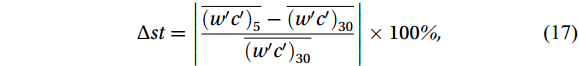
To ensure that the half-hourly turbulence statistics were stable, a turbulence smoothness test was performed using the following expression (Lee et al., 2005):
$$ \Delta st=\left|\frac{\overline{({w}{{'}}{c}{{'}}{)}_{5}}-\overline{({w}{{'}}{c}{{'}}{)}_{30}}}{\overline{({w}{{'}}{c}{{'}}{)}_{30}}}\right|\times 100\text{%} , $$ (17) The subscripts “5” and “30” represent 5 and 30 min samples, respectively, in the same time period.
3.3.3 Turbulence development adequacy
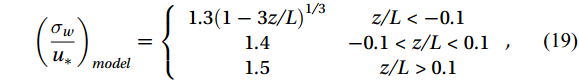
The adequacy of turbulence development can be expressed in terms of the overall turbulence characteristic coefficients (ITC, integral turbulence characteristics). Atmospheric turbulence is considered to be adequately developed if the ITC is < 30% (Kaimal et al., 1972; Lee et al., 2005). The ITC expression is:
$$ \text{IT}{\text{C}}_{\sigma }=\left|\frac{({\sigma }_{w}/{u}_{*}{)}_{\text{model}}-({\sigma }_{w}/{u}_{*}{)}_{\text{measured}}}{({\sigma }_{w}/{u}_{*}{)}_{\text{model}}}\right| , $$ (18) where
$ {\sigma }_{\mathrm{w}} $ is the vertical wind speed variance. The subscripts model and measured denote the modeled and actual measurements, respectively. The empirical relationship between vertical wind speed and friction velocity ratio is given by (Panofsky and Dutton, 1984; Foken et al., 2005):$$ {\left(\frac{{\sigma }_{w}}{{u}_{*}}\right)}_{model}=\left\{\begin{array}{cc}1.3(1-3z/L{)}^{1/3}& z/L < -0.1\\ 1.4& -0.1 < z/L < 0.1\\ 1.5& z/L > 0.1\end{array}\right. , $$ (19) where
$ z $ is the set-up height;$ L $ is the Obukhov length;$ z/L $ is the atmospheric stability factor, which is a dimensionless parameter typically ranging from −5 to 5, with positive (negative) values indicating stable (unstable) values, and values approaching 0 indicate the limit of neutral stratification.The Obukhov length
$ L $ is a parameter that indicates the proportional influence of shear force and bouyancy in the generation and consumption of turbulence kinetic energy:$$ L=-\frac{{{u}_{*}}^{3}\theta }{kg\overline{{w}{\prime}{\theta }{\prime}}} , $$ (20) where
$ k $ is von Kármán’s constant,$ g $ is gravitational acceleration, and$ \theta $ is potential temperature.4. Results and discussion
In this study, data from the offshore platform in August 2020 and the island platform data in July 2021 were used as examples to analyze the air-sea flux observations at different frequencies. Three main aspects were included: data calibration, quality assessment, and differences in air-sea flux observed at different frequencies.
4.1 Data calibration
4.1.1 Time delay
The maximum correlation coefficients of ultrasonic wind speed with water vapor and CO2 concentration were analyzed to determine the delay time using the observation data from the offshore platform, respectively (Fig. 5). The results show the delay times of the ultrasonic anemometer with the high-frequency water vapor pulsometer and the high-frequency CO2 pulsometer are −0.1 s and 1 s, respectively.
 Figure 5. Delay times. Delay time of ultrasonic anemometer with high-frequency CO2 pulsometer (a) and with high-frequency water vapor pulsometer (b).
4.1.2 Coordinate rotation
Figure 6 shows the changes in the 3-D wind speed vector before and after that DR that transforms the 3-D wind speed vector from the ultrasonic anemometer coordinate system to the natural coordinate system. The pre-correction image (a) shows that the vertical wind speed
$ w $ tends to increase as the horizontal wind speed$ u $ and side wind$ v $ decrease. The vertical distance of the measured 3-D wind speed scattering points from the u-v plane shows that$ w $ was generally positive and the direction was upward before correction. After correction (b),$ w $ was uniformly distributed on both sides of the u-v plane so that$ w=0 $ and included upward and downward vertical wind speeds. In addition, the overall vertical distance after correction was smaller than the vertical distance before correction, and the data scatter was uniformly distributed throughout the plane. The results show that the DR method effectively performed the tilt correction and reduced the interference of different wind speed components. Figure 6. Three-dimensional wind speed correction. (a) Before correction; (b) after correction. In the Fig., “○” is the average of 5 min wind speed samples from the offshore platform and the solid line is the vertical distance between “○” and the u-v plane.
4.1.3 Air-sea flux duration
The Ogive curve, which integrates the co-spectrum of the vertical wind speed
$ w $ and physical quantity x from low to high frequencies, was used to verify the adequacy of the air-sea flux averaging duration in capturing all air-sea fluxes. If the Ogive value converges gradually at low frequencies, it indicates that the air-sea flux computation time scale is appropriate (Oncley et al., 1996; Lee et al., 2005).The Ogive curves of downwind and vertical wind speeds plotted for 16 randomly selected days from our July 2021 offshore platform observations, and randomly selecting 1 hour data each day. Each Ogive Curve corresponds to one hour of data from one of the days. We randomly select as much data as possible to ensure that the chosen data can represent the overall data quality. The results in Fig. 7 show that the Ogive value gradually increases over time. When the observation time reaches 1 min, the Ogive value gradually becomes stable; most of the data become completely stable at 5 min, and the Ogive value gradually approaches 1.0 m2/s2 at 30 min. Oncley et al. (1996) analyzed 10 Hz observation samples and found that the optimal observation length was between 5 min and 30 min, and the corresponding natural frequency was 3.3 × 10⁻³ Hz ~ 5.6 × 10⁻⁴ Hz. Unlike previous studies, the air-sea observation frequencies in this study were carried out at 100 Hz, which allowed for the detection of smaller and more frequent changes in turbulence. To analyze the influence of different observation frequencies on the air-sea flux, we examined the observed data of the air-sea fluxes from offshore platforms and islands, with the shortest duration (5 min) in Oncley et al. (1996).
 Figure 7. Ogive curves of downwind and vertical wind speeds plotted for 16 randomly selected days from our July 2021 offshore platform observations, and randomly selecting 1 hour data each day. Each Ogive Curve corresponds to one hour of data from one of the days.
$ z/L= 0 $ .4.1.4 WPL correction
Data in July 10, 2021 were selected as the island observations, which were more comprehensive than the other days, because it was more complete and allowed to analyze flux changes over the course of the day. As mentioned in Section 2.2, the island observations were only high-frequency observations of water vapor. Therefore, in this section, only the air-sea water vapor fluxes were corrected for WPL, and the changes in air-sea flux before and after the correction were analyzed.
Figure 8 shows that in terms of the magnitude of air-sea flux change, the WPL corrected water vapor flux was smaller than the uncorrected water vapor flux, which is consistent with the results of Jentzsch et al. (2021). The difference was that Fig. 8 has two corrected peaks at 09:00 and 19:25 due to the complex island observing environment. In terms of air-sea flux differences, the WPL correction has a significant effect on the calculated values of water vapor fluxes, with a maximum amplitude effect on air-sea fluxes of about 1.5 mmol/(m2·s). The air-sea flux differences before and after the correction varied with time and were significantly different. Between 0:00 and 9:00, the air-sea flux difference showed a clear upward trend; from about 9:00 to 18:10, the air-sea flux difference showed a downward trend accompanied by an increase in amplitude of about 1 h, which maintained a stable air-sea flux difference during the night. The results of the WPL corrections show that temperature and water vapor led to a change in the density of the observed amount, resulting in notable changes in air-sea flux change. The faster the temperature and water vapor changed, the larger the magnitude of the correction.
 Figure 8. Water vapor flux WPL correction (July 10, 2021). Black lines indicate uncorrected air-sea fluxes; solid gray lines indicate corrected results; red dashed lines indicate the difference between pre-correction minus correction, and “//” indicates truncated invalid data.
4.2 Quality assessment
4.2.1 Turbulence spectrum analysis
The wind speed power spectrum and its co-spectrum with CO2 and water vapor are analyzed from selected island observations. Fig. 9 shows that the inertial subregion was in the frequency range of approximately 1 Hz to 10 Hz. The peak value of the power spectrum appears at a frequency lower than 1 Hz, representing a region of high energy content known as the energy-containing vortex region, and the spectrum value in the range from 10–3 to 100 increases with the increase of frequency. When the frequency is about 1 Hz to 10 Hz, the power spectrum shows a downward trend, and the turbulent kinetic energy produces a turbulent cascade with isotropic characteristics. Parallel to the slope line, this part follows the −2/3 law, representing the inertial subregion. When the frequency is higher than 10 Hz, the spectral value change deviates from this slope line, which indicates the onset of the dissipation region. Here, turbulent kinetic energy is transferred to a smaller-scale vortex and dissipates into internal energy due to molecular viscosity.
 Figure 9. Wind speed power spectra. (a), (b), (c) and (d), (e), (f) are the power spectra of offshore platforms and island of
$ u $ ,$ v $ , and$ w $ , respectively; solid gray lines indicate measured data, “○” indicates averaged data, and dashed lines indicate “–2/3” slopes.In stable conditions (–0.1 < z/L≤ 1) at low frequencies, data from offshore platforms shows an upward trend as frequency decreases, while the island data shows a decreasing trend with the decrease of frequency. This opposite trend between the two instruments indicates that the 100 Hz instruments are more capable of capturing detailed changes in the low-frequency region.
Figure 10 shows the co-spectrum of vertical wind speed
$ w $ with CO2 and water vapor. The solid gray line indicates co-spectra of w with H2O (Fig. 10a) and CO2 (Fig. 10b) respectively. And “●” indicates averaged co-spectra data. The gray shading in the Fig. shows the relationship between the raw data and the frequency, and the black dots are quality-controlled averages. In calculating the averaged co-spectra data logarithms with e as the base, while the overall representation of the image is a coordinate system with 10 as the base, which better presents the trend of the data. As shown in Fig. 10, the distribution of the mean values is relatively uniform, and the entire result shows a trend that is generally consistent with the –4/3 slope, especially between frequencies greater than 100 Hz and less than 102 Hz. Figure 10. Co-spectral analysis. (a), (b) are co-spectra of
$ w $ with H2O and CO2, respectively. The solid gray line indicates co-spectra of$ w $ with H2O (Fig. 10a) and CO2 (Fig. 10b) respectively. And “●” indicates averaged co-spectra data, the dashed line indicates the “–4/3” slope; the solid black line indicates the Kaimal et al. (1972) is suitable for atmospheric stabilization.The measured mean data were most consistent with the Kaimal et al. (1972) atmospheric instability (–1.0 < z/L ≤ –0.1) in the low-frequency region, and the trend of the scatter distribution in the high-frequency region was more consistent with the –4/3 slope. At frequencies less than 0.01 Hz, the co-spectral values were higher than those of Kaimal’s results due to factors such as insufficient sample data and noise. At frequencies higher than 10 Hz, small co-spectral densities may lead to larger measurement errors (Su et al., 2004). Combining the power spectrum and co-spectrum results, the high-frequency observations fulfil the power spectrum slope of –2/3 and the co-spectrum slope of –4/3 in the inertial sub-region.
4.2.2 Overall quality assessment
Due to the short time series of the offshore platform observation data, which is not conducive to turbulence quality analysis, the island observation data were used to evaluate the overall turbulence quality of the air-sea fluxes and assess the overall quality of the water vapor flux data with three grades of 0, 1, and 2 (see Table 3).
Figure 11 shows the overall turbulence data quality after the turbulence smoothness test and the turbulence development adequacy test. The results show that high-quality data account for about 46.5% of the overall air-sea flux data, and 25.0% of the moderate-quality data. About 28.5% of the points to be discarded were distributed around 12:00 on July 10 and 11. Overall about 71.5% of the island water vapor flux data passed the turbulence smoothness test and the turbulence development adequacy test. In Fig. 11 around 14:00 on July 11, there is a data point with a value of 5 mmol/(m2·s) and QC = 1, which means that this is the general quality data, and around 20:00 in the evening of July 11, the water vapor flux has a value of –3 mmol/(m2·s) and QC = 2, which means that it is the low-quality data. It can be seen that the QC = 1 data interval used for the general quality analysis is quite scattered, with a large difference between the maximum and minimum values.
 Figure 11. Overall turbulence data quality for island water vapor flux observations. “■” denotes high quality data; “▼” denotes moderate quality data; “×” denotes invalid data.
4.3 High/low frequency comparison
Figure 12 shows the air-sea flux observations from the offshore platform. The 100 Hz and 20 Hz air-sea flux trends were generally the same but with larger variations. Water vapor fluxes showed opposite trends for the high and low-frequency observations from 14:55 to 15:05 (Fig. 12a). This may be related to the fact that more turbulent changes are monitored by high-frequency observations, and it is normal for air-sea flux trends to be reversed on smaller timescale scales. At 16:45, the CO2 flux had a negative air-sea flux in high-frequency measurements and a positive flux in low-frequency measurements (Fig. 12b). These results indicate that the measurement frequency had an important effect on the air-sea flux, affecting both intensity and direction.
 Figure 12. Air-sea flux observations from offshore platforms. (a) is the water vapor flux and (b) is the CO2 flux. “▼” denotes 100 Hz frequency; “●” denotes 20 Hz frequency; dashed line denotes zero air-sea flux.
Figure 13a shows the difference between the high and low-frequency water vapor fluxes. These air-sea fluxes were small and less than 0.01 mmol/(m2·s) on July 9, while the difference between the fluxes on July 10 and 11 increased from about 0.005 to 0.03 mmol/(m2·s). According to the experimental record, there was rain on the island on July 10 and 11, which increased the water vapor density in the air and subsequently the air-sea fluxes. Figs. 13b, c, and d show the local magnification of the water vapor flux variations on July 9, 10, and 11, respectively. During this time, the water vapor fluxes varied between –0.2 and 1.00 mmol/(m2·s), with total air-sea fluxes being positive. From 15:21 to 15:43 on July 11, the air-sea flux peaks were lower in the high-frequency observations than in the low-frequency observations. An opposite trend was observed at 15:00 observation at the offshore platform (Fig. 12a). These two fluxes are not directly correlated and have different response rates for different concentrations in air, the source-sink variations in H2O and CO2 fluxes are not in one-to-one correspondence. During the field measurements, the weather and instrument shaking conditions were the same, and the performance was stable except for a sudden drop in the CO2 values at 15:00. This inconsistency in the sudden change may be due to the fact that the two fluxes were measured at some distance from each other in the field, which had a certain impact on the results. In addition to this, it can also be shown that this difference was caused by high-frequency observations that were able to capture additional information about turbulence changes, both upward and downward, on a different timescale. Taken together, the frequency of the observations had a smaller effect on the water vapor flux than on the CO2 flux, probably because the water vapor concentration in the atmosphere was much higher than the CO2 concentration.
 Figure 13. Comparison of observed air-sea fluxes at different frequencies over the island. (a) Difference between 100 Hz and 20 Hz air-sea fluxes; (b), (c), and (d) are partial zoomed-in plots showing island air-sea flux observations on July 9, 10, and 11, 2021, respectively. The “//” denotes the axes of the truncated, partially invalid data, “▼” denotes 100 Hz, and “●” denotes 20 Hz.
Figure 14 shows the evolution over time of water vapor and CO2 concentrations. The high-frequency observations had more pulsed values and more pronounced amplitudes of change than the low-frequency observations. Observations from the offshore platform were smooth, with high water vapor concentrations and narrow variations. Long-term observations on the islands showed some cyclical variations in water vapor concentration, with a sudden drop in water vapor concentration on July 11. This systematic and abrupt change can be attributed to factors such as changes in meteorological conditions and sensor drift (Moncrieff et al., 2004). The change in the trend of the data from the offshore platforms was not as obvious. There is a downward trend in the data from the platforms on the islands. In terms of the overall performance of the data, the high-frequency observations were able to monitor more of the small changes in the turbulence than the low-frequency data.
 Figure 14. Water vapor and CO2 concentrations over time; (a) and (b) are water vapor versus time for offshore platform and island data, respectively. The inner image of (a) is its local zoom; (c) is the CO2 variation with time. The red solid line indicates 100 Hz observations and the black solid line indicates 20 Hz observations.
Figure 15 comprehensively shows the variation of air-sea fluxes between the island and offshore platforms with wind speed. Despite higher overall wind speeds at the offshore compared to that of the offshore platform, their air-sea fluxes show opposite behaviors. One difference is that the air-sea flux varies in size; second, the trends in air-sea flux change differ. These air-sea fluxes are determined by two factors: wind speed and gas concentration. In the nearshore seas, the proximity to land promotes frequent gas exchange, resulting in a higher variability in air-sea flux values. The air-sea flux on the offshore platform decreases with increasing wind speed, while on the island, air-sea flux increases with the increase of wind speed. These results show that with higher wind speeds, the island environment has more vertical turbulence than the offshore platform, leading to increased atmospheric instability increases. As wind speed increases, the error in air-sea flux measurements also increases. There is no significant difference observed in measurement errors between high-frequency and low-frequency measurements. However, as wind speed increases, the difference in air-sea flux between the high and low-frequency measurements on the two platforms becomes more pronounced.
 Figure 15. Island and nearshore air-sea fluxes vary with wind speed; red dots indicate 100 Hz observed air-sea fluxes, black squares indicate 20 Hz observed air-sea fluxes; error bars indicate 95% confidence intervals.
In Fig. 16, it is evident that water vapor fluxes from offshore platforms exhibit an inverse trend to CO2 fluxes, and opposite to the variation trend of water vapor flux on the islands. The water vapor flux of the offshore platform decreases with the increase in wind speed, and the water vapor flux value ranges from −0.1 mmol/(m2·s) to 0.2 mmol/(m2·s), while the wind speed ranges from 8 m/s to 11 m/s, indicating low and intermediate wind speeds. The ambient water vapor flux ranges from −0.2 mmol/(m2·s) to 1 mmol/(m2·s), and the wind speed ranges from 0 m/s to 8 m/s. The overall water vapor flux direction of the island environment trends upward, while the water vapor flux of the offshore platform is balanced and the water vapor exchange is weak. For CO2 flux, the overall air-sea flux direction trends upward, and the ocean is the source of CO2 release. In obtaining this result, we did not take into account the problem of the distance from the installation position of the instrument, and we hope to further improve the accuracy of our results in subsequent experiments. In terms of basic variation trends and errors, the results in Fig. 16 are consistent with those in Fig.15.
 Figure 16. Trends and confidence analyses of air-sea CO2 and water vapor fluxes; red dots indicate 100 Hz air-sea flux data, blue dots indicate 20 Hz air-sea flux data; red and blue lines indicate fitted curves; and shaded areas indicate 95% confidence limits.
The above results show that the trends of variation in air-sea flux with wind speeds are notably different due to differences in the underlying surface environment and atmospheric stability. With the increase of wind speed, the air-sea flux measurement error increases, so the uncertainty of observation frequency to air-sea flux increases. However, the overall difference between 100 Hz and 20 Hz errors is not large, and the observed air-sea flux values are different.
There are few reports on gas analyzers at 100 Hz, and there is no fixed relationship between air-sea CO2 and water vapor flux and wind speed. This is because wind speed mainly changes the transfer velocity without altering the magnitude of the partial pressures of CO2 or water vapor. The carbon source or sink primarily depends on the difference in CO2 partial pressure between the atmosphere and seawater. If the atmospheric CO2 partial pressure is greater, the ocean acts as a carbon sink, and if the ocean's CO2 partial pressure is greater, the ocean acts as a carbon source. The difference in CO2 partial pressure varies across different regions, hence the relationship between flux and wind speed will differ. This paper mainly aims to illustrate the differences in air-sea CO2 and water vapor flux observed at 20 Hz and 100 Hz, as well as the fact that high-frequency observations are superior to low-frequency observations under high wind speed conditions, through Fig. 16. The work of Li et al. (2021b) can support our conclusion.
Changes in turbulence occur very quickly, and thus concentrations and densities change accordingly. It is therefore necessary to use instruments with high accuracy and fast measurement data transfer rates, especially in windy environments. (1) Due to the limitation of low frequency of observation instruments, it often happens that the inertial domain band of the measured spectrum is too narrow to fit the Kolmogorov-5/3 power law well. The turbulence energy spectrum obtained from high-frequency observation covers not only the inertial subregion, but also part of the viscous subregion, which is conducive to calculating the turbulence parameters more accurately, and to identifying and analyzing turbulence characteristics. (2) When using Ogive Curves to calculate the averaging time, low-frequency observations may mask or smooth out some transient features of turbulence, while high-frequency observations can reduce this effect and make the observations closer to the real situation. Also, due to the intermittent nature of turbulence, turbulent and non-turbulent layers that are clearly bounded in low-frequency observations may underestimate certain fluxes. High-frequency observations can reduce this underestimation by capturing more turbulent activity, estimating turbulent fluxes more accurately, and tracking transient changes in turbulence. In addition to this, high-frequency observations provide data with higher temporal resolution, which page means that rapid changes in turbulence over time can be observed in more detail.
5. Conclusion
In this paper, we used water vapor and CO2 flux observations from offshore platforms and island platforms to carry out comprehensive data calibration and data quality, focusing on the effects of 100 and 20 Hz observing frequencies on air-sea flux observations. Different durations between different frequencies were found to have a great influence on the air-sea flux calculations. We chose a duration of 5 min for these calculations. Based on the results of the turbulence spectrum analysis, turbulence smoothness, and turbulence development adequacy tests, the observed data met the requirements for accurate air-sea flux calculations. The temperature and water vapor density corrections reduced the air-sea flux magnitude to some extent, and further reduced the air-sea flux differences caused by different observation frequencies. At low wind speeds, there were more high-frequency observations with different air-sea flux magnitudes and directions than low-frequency observations. The frequency of the wind speed observations was not the main factor contributing to the air-sea flux differences; rather, it was the magnitude of wind speed that contributed to the differences between high and low-frequency observations. At high wind speeds, the difference between high and low-frequency water vapor fluxes was small, and there was an overall large difference in CO2 fluxes. The results regarding the effects of environmental factors such as wind speed, temperature, and water vapor on the air-sea fluxes under high-frequency and low-frequency observations showed that high-frequency observations could provide more detailed information on turbulence variations than low-frequency data. Furthermore, changes in the air-sea fluxes of gases with lower concentrations in the atmosphere could be observed on short time scales.
-
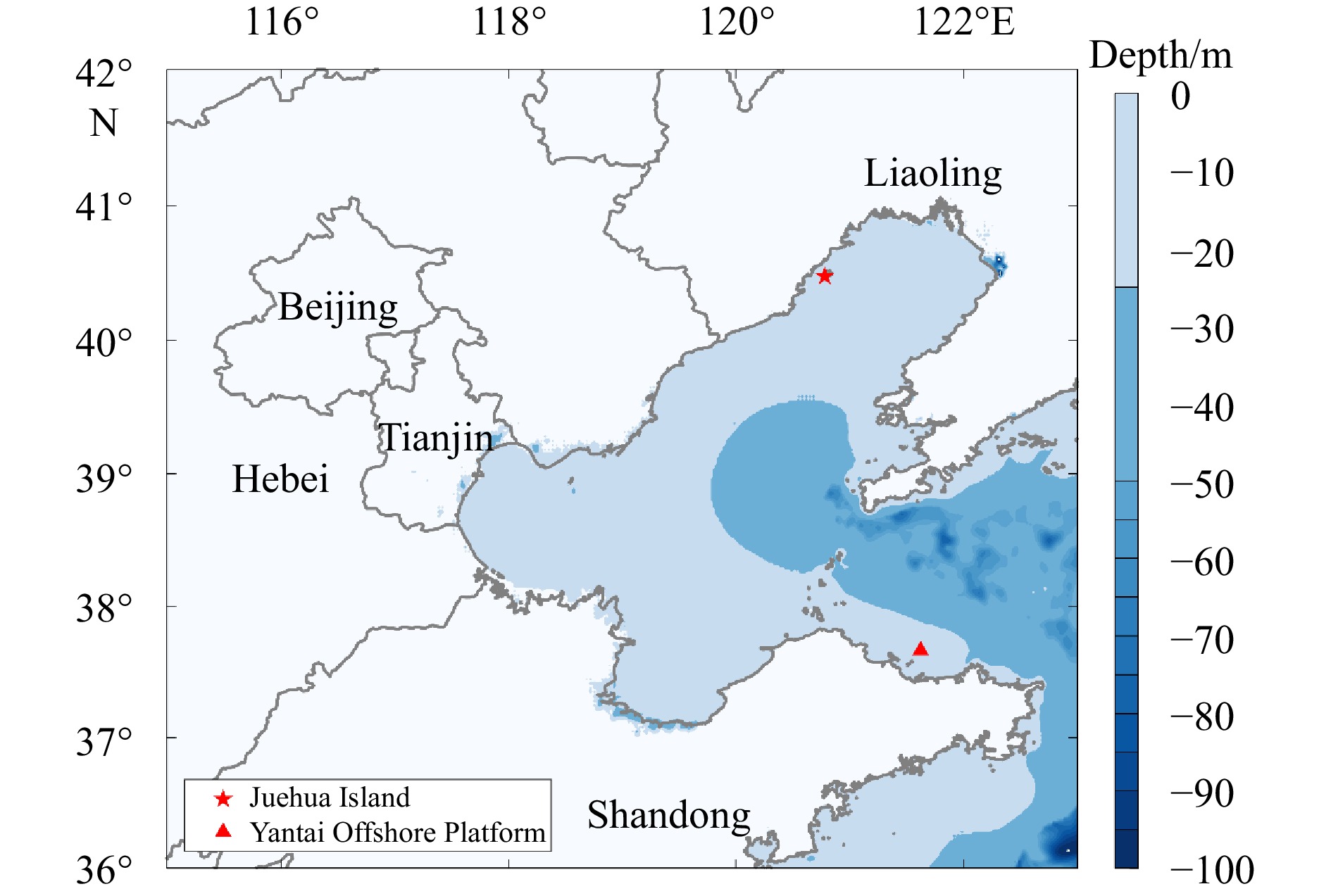
Figure 1. Air-sea flux observation platforms. Symbol‘★’is the observation platform of Juehua Island, and‘▲’is the Yantai National Satellite Ocean Calibration Platform.
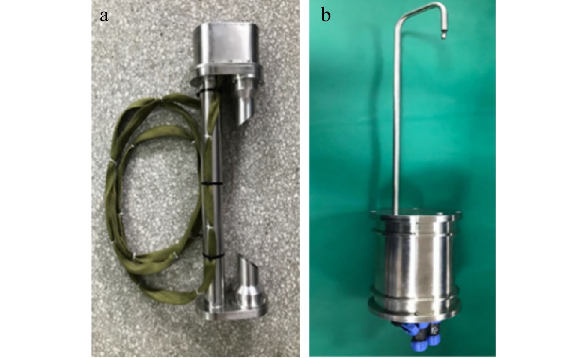
Figure 2. High-frequency 100 Hz pulsating gas analyzer. (a) CO2 gas analyzer; (b) H2O gas analyzer.

Figure 3. In situ observation experiments. (a) and (b) are the Yantai National Satellite Ocean Calibration Platform and the island observation platform at Juehua Island, Liaoning Province, respectively; (c) and (d) are the instrumentation of platforms (a) and (b), respectively.

Figure 4. Raw data preprocessing and air-sea flux calculation flow chart. The dashed boxes represent steps that are not included in the main air-sea flux calculation process and are discussed separately in this article.
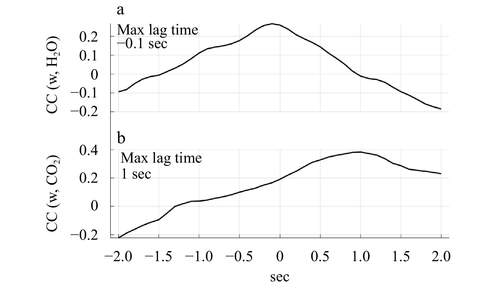
Figure 5. Delay times. Delay time of ultrasonic anemometer with high-frequency CO2 pulsometer (a) and with high-frequency water vapor pulsometer (b).

Figure 6. Three-dimensional wind speed correction. (a) Before correction; (b) after correction. In the Fig., “○” is the average of 5 min wind speed samples from the offshore platform and the solid line is the vertical distance between “○” and the u-v plane.
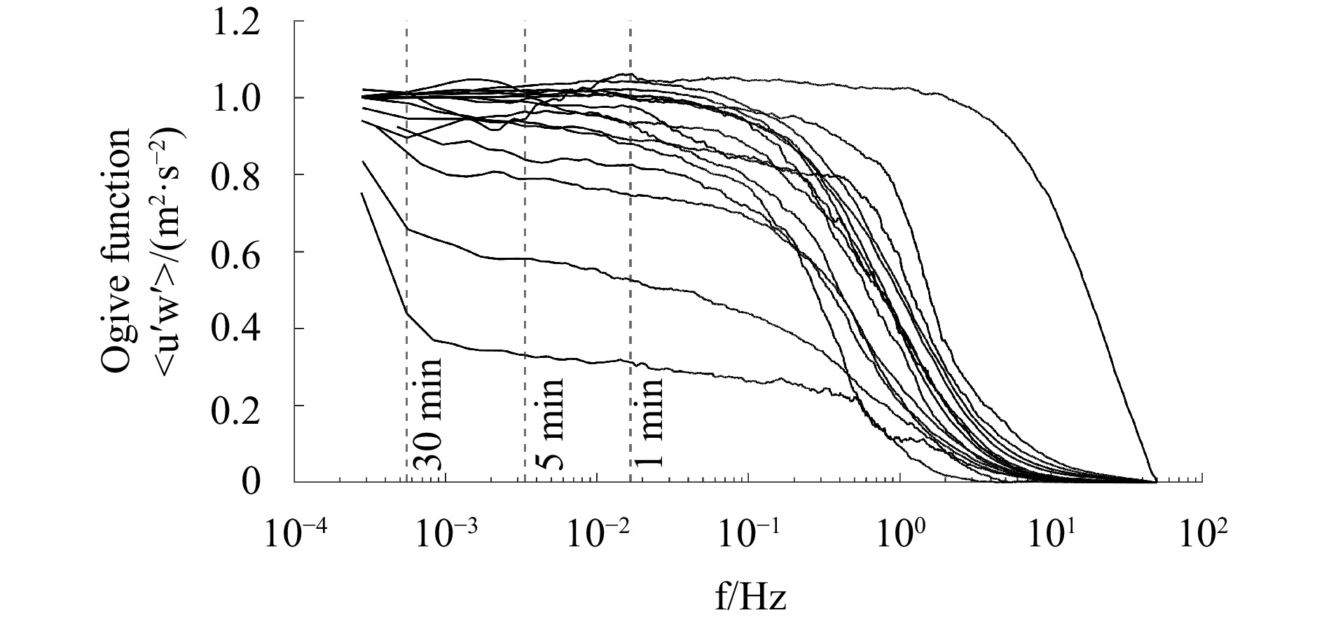
Figure 7. Ogive curves of downwind and vertical wind speeds plotted for 16 randomly selected days from our July 2021 offshore platform observations, and randomly selecting 1 hour data each day. Each Ogive Curve corresponds to one hour of data from one of the days.
$ z/L= 0 $ .
Figure 8. Water vapor flux WPL correction (July 10, 2021). Black lines indicate uncorrected air-sea fluxes; solid gray lines indicate corrected results; red dashed lines indicate the difference between pre-correction minus correction, and “//” indicates truncated invalid data.
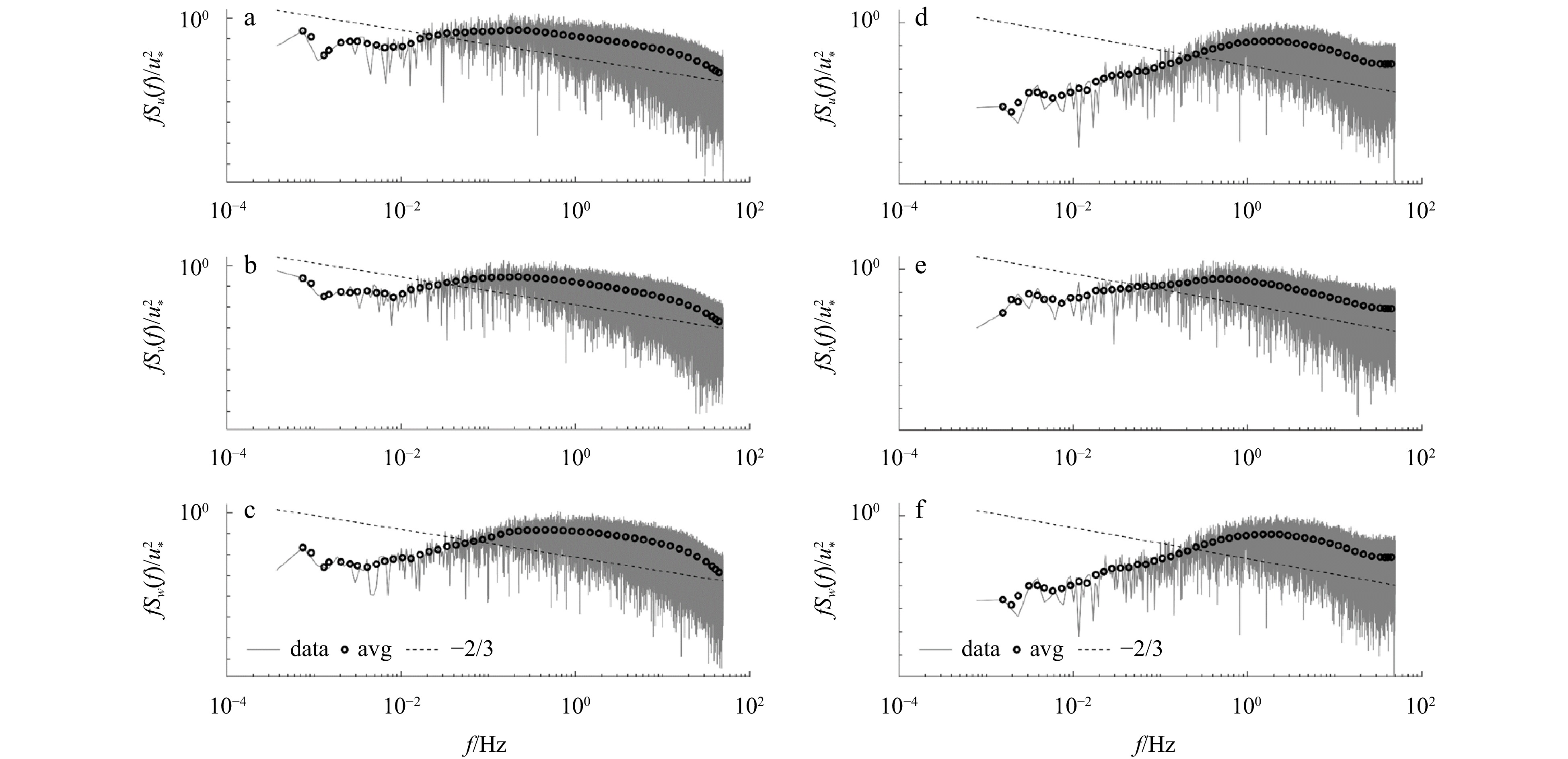
Figure 9. Wind speed power spectra. (a), (b), (c) and (d), (e), (f) are the power spectra of offshore platforms and island of
$ u $ ,$ v $ , and$ w $ , respectively; solid gray lines indicate measured data, “○” indicates averaged data, and dashed lines indicate “–2/3” slopes.
Figure 10. Co-spectral analysis. (a), (b) are co-spectra of
$ w $ with H2O and CO2, respectively. The solid gray line indicates co-spectra of$ w $ with H2O (Fig. 10a) and CO2 (Fig. 10b) respectively. And “●” indicates averaged co-spectra data, the dashed line indicates the “–4/3” slope; the solid black line indicates the Kaimal et al. (1972) is suitable for atmospheric stabilization.
Figure 11. Overall turbulence data quality for island water vapor flux observations. “■” denotes high quality data; “▼” denotes moderate quality data; “×” denotes invalid data.

Figure 12. Air-sea flux observations from offshore platforms. (a) is the water vapor flux and (b) is the CO2 flux. “▼” denotes 100 Hz frequency; “●” denotes 20 Hz frequency; dashed line denotes zero air-sea flux.
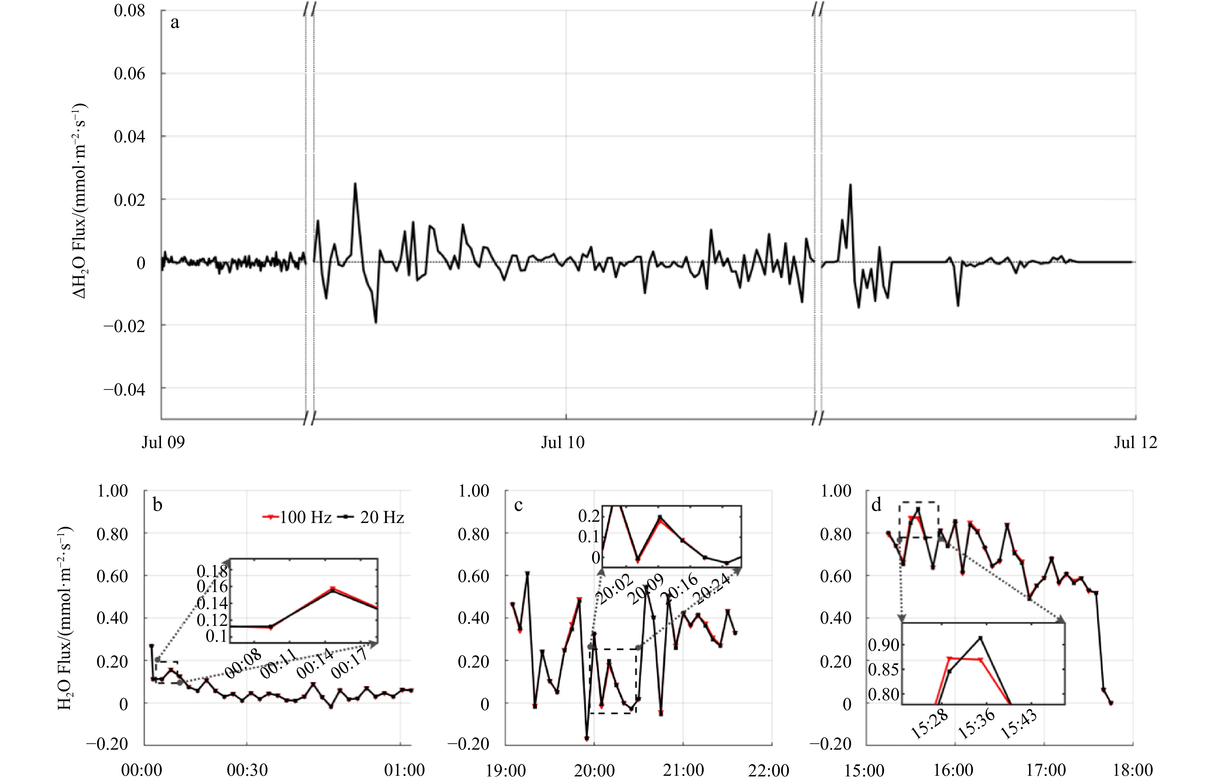
Figure 13. Comparison of observed air-sea fluxes at different frequencies over the island. (a) Difference between 100 Hz and 20 Hz air-sea fluxes; (b), (c), and (d) are partial zoomed-in plots showing island air-sea flux observations on July 9, 10, and 11, 2021, respectively. The “//” denotes the axes of the truncated, partially invalid data, “▼” denotes 100 Hz, and “●” denotes 20 Hz.
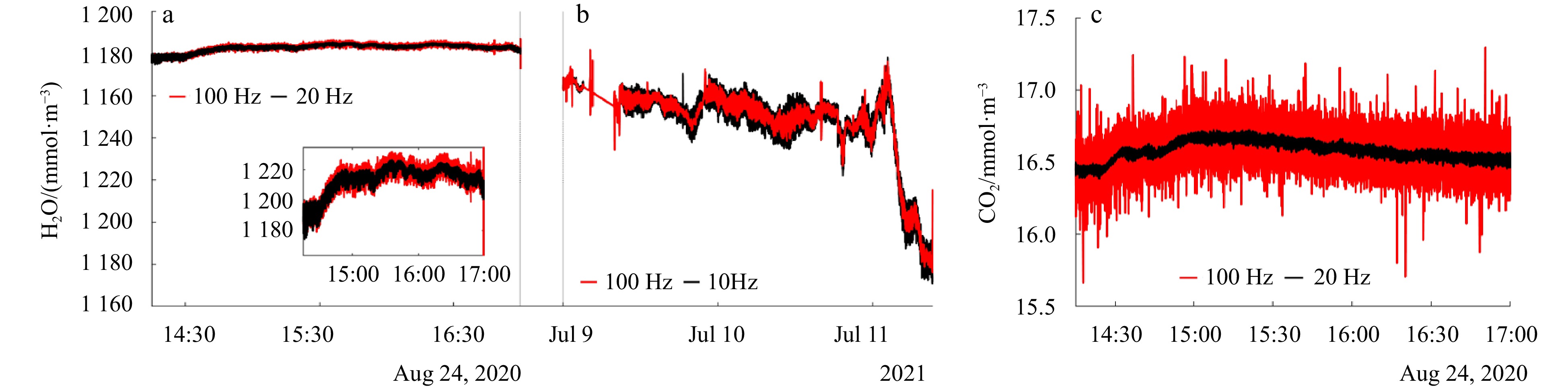
Figure 14. Water vapor and CO2 concentrations over time; (a) and (b) are water vapor versus time for offshore platform and island data, respectively. The inner image of (a) is its local zoom; (c) is the CO2 variation with time. The red solid line indicates 100 Hz observations and the black solid line indicates 20 Hz observations.
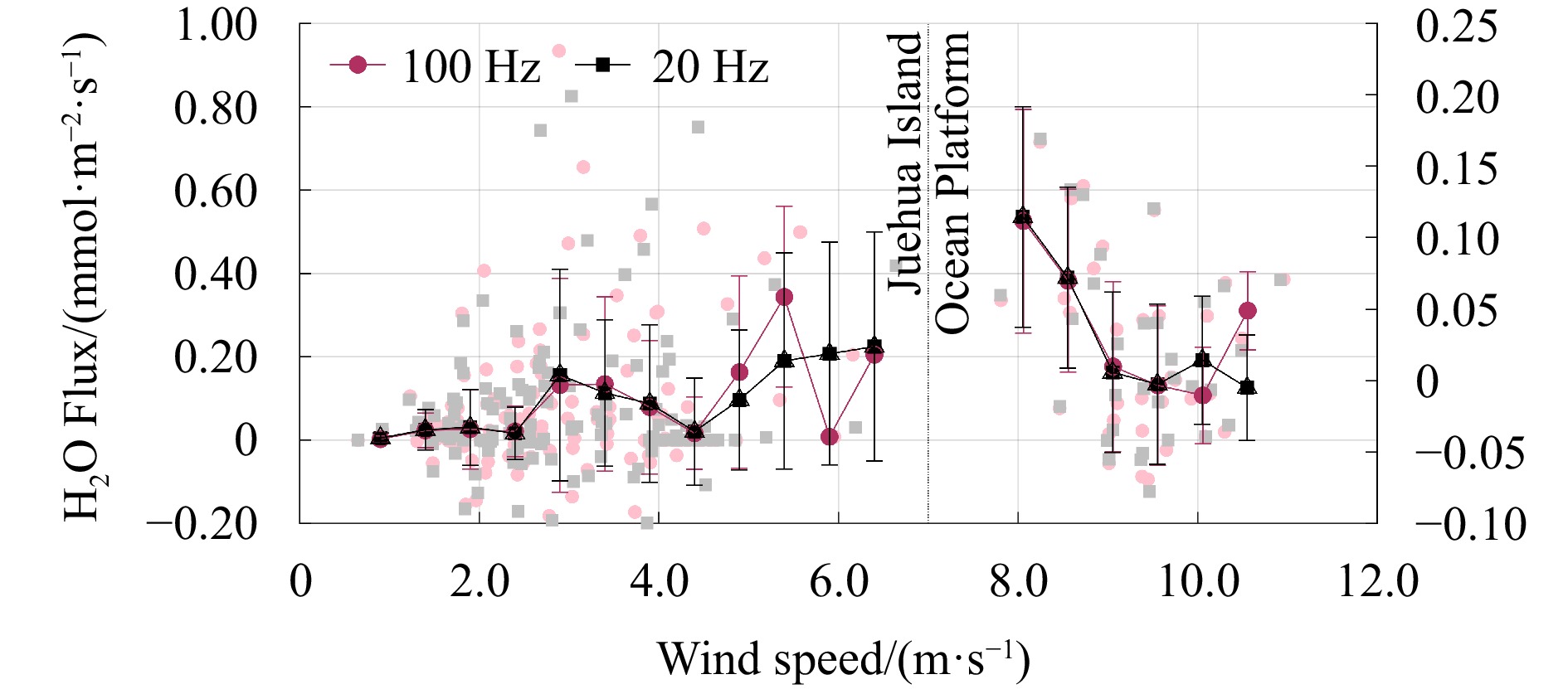
Figure 15. Island and nearshore air-sea fluxes vary with wind speed; red dots indicate 100 Hz observed air-sea fluxes, black squares indicate 20 Hz observed air-sea fluxes; error bars indicate 95% confidence intervals.

Figure 16. Trends and confidence analyses of air-sea CO2 and water vapor fluxes; red dots indicate 100 Hz air-sea flux data, blue dots indicate 20 Hz air-sea flux data; red and blue lines indicate fitted curves; and shaded areas indicate 95% confidence limits.
Table 1. Measuring range of Ultrasonic anemometer
Instrument
/parameterWind speed range Wind speed accuracy Wind direction range Wind accuracy Measuring frequency Installation
siteHS-100 0-45 m/s <1.0% RMS 0-359° <±1.0°RMS 100 Hz Island & Platform  下载: 导出CSV
Table 2. Measuring range of CO2/H2O gas analyzer
Instrument/parameter Concentration Measuring frequency Installation site Licor-7500A 0—50 mmol/mol
0—3 000 10–610 Hz Island Licor-7500DS 0—50 mmol/mol
0—3 000 10–620 Hz Platform *CO2/H2O High frequency pulsometer * 100 Hz Island & platform Note: The symbol “*” indicates that the measuring range is limited by reference to the Licor measuring range.
下载: 导出CSV
Table 3. Turbulence data quality classification standards.
Turbulence stability (%) Turbulence development adequacy (%) overall quality level <30 <30 0 <100 <100 1 >100 >100 2 Note: * Level 0 is high quality data that can be used for basic research analysis; Grade 1 is medium quality data, which can be used for general air-sea flux analysis; Level 2 is low-quality data and should be discarded or interpolated.
下载: 导出CSV
-
Baldocchi D D. 2003. Assessing the eddy covariance technique for evaluating carbon dioxide exchange rates of ecosystems: past, present and future. Global Change Biology, 9(4): 479–492, doi: 10.1046/j.1365-2486.2003.00629.x Baldocchi D D, Hincks B B, Meyers T P. 1988. Measuring biosphere-atmosphere exchanges of biologically related gases with micrometeorological methods. Ecology, 69(5): 1331–1340, doi: 10.2307/1941631 Blomquist B W, Fairall C W, Huebert B J, et al. 2012. Direct measurement of the oceanic carbon monoxide flux by eddy correlation. Atmospheric Measurement Techniques, 5(12): 3069–3075, doi: 10.5194/amt-5-3069-2012 Brevik E C. 2012. Soils and climate change: gas fluxes and soil processes. Soil Horizons, 53(4): 12–23, doi: 10.2136/sh12-04-0012 Burba G. 2013. Eddy Covariance Method: for Scientific, Industrial, Agricultural, and Regulatory Applications: A Field Book on Measuring Ecosystem Gas Exchange and Areal Emission Rates. Lincoln: LI-COR Biosciences, 22–25 Coe D, W. Fabinski, G. Wiegleb. 2021. The impact of CO2, H2O and other “greenhouse gases” on equilibrium earth temperatures. International Journal of Atmospheric and Oceanic Sciences, 5(2): 29–40., doi: 10.11648/j.ijaos.20210502.12 Czubaszek R, Wysocka-Czubaszek A. 2023. Temporal dynamics of CO2 fluxes measured with eddy covariance system in maize, winter oilseed rape and winter wheat fields. Atmosphere, 14(2): 372, doi: 10.3390/atmos14020372 Else B G T, Papakyriakou T N, Galley R J, et al. 2011. Wintertime CO2 fluxes in an Arctic polynya using eddy covariance: evidence for enhanced air-sea gas transfer during ice formation. Journal of Geophysical Research: Oceans, 116(C9): C00G03 Eugster W, Burkard R, Klemm O, et al. 2001. Fog deposition measurements with the eddy covariance method. In: Schemenauer R, Puxbaum H, eds. Proceedings of the Second International Conference on Fog and Fog Collection. St. John’s, Canada: 193–196 Foken T, Göockede M, Mauder M, et al. 2005. Post-field data quality control. In: Lee Xuhui, Massman W, Law B, eds. Handbook of Micrometeorology: A Guide for Surface Flux Measurement and Analysis. Dordrecht: Springer, 181–208 Geernaert G L. 1988. Measurements of the angle between the wind vector and wind stress vector in the surface layer over the North Sea. Journal of Geophysical Research: Oceans, 93(C7): 8215–8220, doi: 10.1029/JC093iC07p08215 Hart S C. 2006. Potential impacts of climate change on nitrogen transformations and greenhouse gas fluxes in forests: a soil transfer study. Global Change Biology, 12(6): 1032–1046, doi: 10.1111/j.1365-2486.2006.01159.x Højstrup J. 1993. A statistical data screening procedure. Measurement Science and Technology, 4(2): 153–157, doi: 10.1088/0957-0233/4/2/003 Horst T W. 2000. On frequency response corrections for eddy covariance flux measurements. Boundary-Layer Meteorology, 94(3): 517–520, doi: 10.1023/A:1002427517744 Hu Enzhu, Babcock E L, Bialkowski S E, et al. 2014. Methods and techniques for measuring gas emissions from agricultural and animal feeding operations. Critical Reviews in Analytical Chemistry, 44(3): 200–219, doi: 10.1080/10408347.2013.843055 IPCC. 2023. Climate Change 2023: Synthesis Report. Geneva, Switzerland: IPCC,119–130 Jentzsch K, Boike J, Foken T. 2021. Importance of the Webb, Pearman, and Leuning (WPL) correction for the measurement of small CO2 fluxes. Atmospheric Measurement Techniques, 14(11): 7291–7296, doi: 10.5194/amt-14-7291-2021 Kaimal J C, Wyngaard J C, Izumi Y, et al. 1972. Spectral characteristics of surface-layer turbulence. Quarterly Journal of the Royal Meteorological Society, 98(417): 563–589 Kaye J P, Quemada M. 2017. Using cover crops to mitigate and adapt to climate change. A review. Agronomy for Sustainable Development, 37(1): 4, doi: 10.1007/s13593-016-0410-x Kondo F, Tsukamoto O. 2007. Air-sea CO2 flux by eddy covariance technique in the equatorial Indian Ocean. Journal of Oceanography, 63(3): 449–456, doi: 10.1007/s10872-007-0040-7 Landwehr S, Miller S D, Smith M J, et al. 2018. Using eddy covariance to measure the dependence of air–sea CO2 exchange rate on friction velocity. Atmospheric Chemistry and Physics, 18(6): 4297–4315, doi: 10.5194/acp-18-4297-2018 Lee Xuhui, Massman W, Law B. 2005. Handbook of Micrometeorology: A Guide for Surface Flux Measurement and Analysis. Dordrecht: Springer, 94–193 Li Shuo, Babanin A V, Qiao Fangli, et al. 2021a. Laboratory experiments on CO2 gas exchange with wave breaking. Journal of Physical Oceanography, 51(10): 3105–3116 Li Mingxing, Kan Ruifeng, He Yabai, et al. 2021b. Development of a laser gas analyzer for fast CO2 and H2O flux measurements utilizing derivative absorption spectroscopy at a 100 Hz data rate. Sensors, 21(10): 3392, doi: 10.3390/s21103392 Liu Shuo, Liu Gang, Zhang Mi, et al. 2022. Evaluation of eddy covariance footprint models through the artificial line source emission of methane. Journal of Geophysical Research: Atmospheres, 127(16): e2021JD036294, doi: 10.1029/2021JD036294 Mammarella I, Launiainen S, Gronholm T, et al. 2009. Relative humidity effect on the high-frequency attenuation of water vapor flux measured by a closed-path eddy covariance system. Journal of Atmospheric and Oceanic Technology, 26(9): 1856–1866, doi: 10.1175/2009JTECHA1179.1 Matthews B, Schume H. 2022. Tall tower eddy covariance measurements of CO2 fluxes in Vienna, Austria. Atmospheric Environment, 274: 118941, doi: 10.1016/j.atmosenv.2022.118941 Mauder M, Foken T. 2015. Documentation and Instruction Manual of the Eddy-Covariance Software Package TK3. Bayreuth: Arbeitsergebnisse, Universität Bayreuth, Abteilung Mikrometeorologie, 67 Miller S D, Hristov T S, Edson J B, et al. 2008. Platform motion effects on measurements of turbulence and air–sea exchange over the open ocean. Journal of Atmospheric and Oceanic Technology, 25(9): 1683–1694, doi: 10.1175/2008JTECHO547.1 Miller S D, Marandino C, Saltzman E S. 2010. Ship-based measurement of air-sea CO2 exchange by eddy covariance. Journal of Geophysical Research: Atmospheres, 115(D2): D02304 Moncrieff J, R Clement, J Finnigan, et al. 2004. Averaging, Detrending, and Filtering of Eddy Covariance Time Series. In: Lee X, Massman W, Law B, eds. Handbook of Micrometeorology: A Guide for Surface Flux Measurement and Analysis. Dordrecht: Springer, Dordrecht Oncley S P, Friehe C A, Larue J C, et al. 1996. Surface-layer fluxes, profiles, and turbulence measurements over uniform terrain under near-neutral conditions. Journal of the Atmospheric Sciences, 53(7): 1029–1044, doi: 10.1175/1520-0469(1996)053<1029:SLFPAT>2.0.CO;2 Palatella L, Rana G, Vitale D. 2014. Towards a flux-partitioning procedure based on the direct use of high-frequency eddy-covariance data. Boundary-Layer Meteorology, 153(2): 327–337, doi: 10.1007/s10546-014-9947-x Panofsky H A, Dutton J A. 1984. Atmospheric Turbulence: Models and Methods for Engineering Applications. New York: Wiley Rannik Ü, Vesala T. 1999. Autoregressive filtering versus linear detrending in estimation of fluxes by the eddy covariance method. Boundary-Layer Meteorology, 91(2): 259–280, doi: 10.1023/A:1001840416858 Rytwo G, Eliyahou D. 2023. Eddy correlation measurements to visualize CO2 and water vapor concentrations and fluxes. Journal of Agrometeorology, 25(2): 239–246, doi: 10.54386/jam.v25i2.2103 Shahan Julie, Chu Housen, Windham-Myers L, et al. 2022. Combining eddy covariance and chamber methods to better constrain CO2 and CH4 fluxes across a heterogeneous restored tidal wetland. Journal of Geophysical Research: Biogeosciences, 127(9): e2022JG007112, doi: 10.1029/2022JG007112 Shukla P R, J Skea, E Calvo Buendia, et al. 2019. IPCC, 2019: Climate Change and Land: an IPCC special report on climate change, desertification, land degradation, sustainable land management, food security, and greenhouse gas fluxes in terrestrial ecosystems. Siebicke L, Emad A. 2019. True eddy accumulation trace gas flux measurements: proof of concept. Atmospheric Measurement Techniques, 12(8): 4393–4420, doi: 10.5194/amt-12-4393-2019 Stagakis S, Feigenwinter C, Vogt R, et al. 2023. A high-resolution monitoring approach of urban CO2 fluxes. Part 1-bottom-up model development. Science of the Total Environment, 858: 160216, doi: 10.1016/j.scitotenv.2022.160216 Su Hongbing, Schmid H P, Grimmond C S B, et al. 2004. Spectral characteristics and correction of long-term eddy-covariance measurements over two mixed hardwood forests in non-flat terrain. Boundary-Layer Meteorology, 110(2): 213–253, doi: 10.1023/A:1026099523505 Swinbank W C. The measurement of vertical transfer of heat and water vapor by eddies in the lower atmosphere[J]. Journal of Atmospheric Sciences, 1951, 8(3): 135-145. Vickers D, Mahrt L. 1997. Quality control and flux sampling problems for tower and aircraft data. Journal of Atmospheric and Oceanic Technology, 14(3): 512–526, doi: 10.1175/1520-0426(1997)014<0512:QCAFSP>2.0.CO;2 Weber R O. 1999. Remarks on the definition and estimation of friction velocity. Boundary-Layer Meteorology, 93(2): 197–209, doi: 10.1023/A:1002043826623 Wilczak J M, Oncley S P, Stage S A. 2001. Sonic anemometer tilt correction algorithms. Boundary-Layer Meteorology, 99(1): 127–150, doi: 10.1023/A:1018966204465 Wuebbles D J, Grant K E, Connell P S, et al. 1989. The role of atmospheric chemistry in climate change. JAPCA, 39(1): 22–28, doi: 10.1080/08940630.1989.10466502 -

 DownLoad:


 点击查看大图
计量
- 文章访问数: 52
- HTML全文浏览量: 19
- 被引次数: 0

