

Population structure and genetic diversity of hairfin anchovy (Setipinna tenuifilis) revealed by microsatellite markers
-
Abstract: Microsatellite markers with polymorphic advantages are widely used in the exploration and utilization of marine fishery resources. In this study, 16 polymorphic microsatellite markers were used to evaluate the diversity and population structure of Setipinna tenuifilis, a nearshore fish of economic and ecological value in the western Pacific and Indian Oceans. The genetic diversity of S. tenuifilis showed a high level (mean Na=23.25, mean Ho=0.639, mean Ra=11.625, and PIC=0.844) similar to other Clupeiformes fish species. The nine wild S. tenuifilis populations showed significant differentiation (FST ranging from
0.00384 to0.19346 ) and were generally divided into southern and northern populations based on genetic structure, except for the Zhoushan population, which exhibited genetic mixture. Our results provide fundamental but significant genetic insights for the management and conservation of S. tenuifilis fishery resources.-
Key words:
- microsatellite /
- population structure /
- genetic diversity /
- Setipinna tenuifilis
-
1. Introduction
Marine environments feature open water, so marine fish are generally considered to have higher genetic diversity and lower genetic differentiation due to facilitated gene exchange. However, an increasing number of population genetics studies have shown that significant genetic differentiation is detected in some marine fishes with large population sizes and extensive habitats, such as Collichtys lucidus (Song et al., 2019), Lateolabrax maculatus (Wang et al., 2021), and Sillago japonica (Han et al., 2021). This suggests that we should master the genetic structure of marine fish as early as possible to deal with the challenges of fishing pressure, climate change, pollution and other challenges.
Setipinna tenuifilis, commonly known as hairfin anchovy, is a pelagic fish with important economic and ecological significance (Li et al., 2022). It has extensive habitats, in the western Pacific and Indian Oceans, and has been recorded in the Bohai Sea, Yellow Sea, East China Sea, and South China Sea of China. In recent years, due to the increase in fishing intensity and the lack of management measures, S. tenuifilis germplasm resources have declined significantly, and people have begun to pay attention to the development and utilization of the S. tenuifilis fishery resources. In order to accurately assess the current status of S. tenuifilis germplasm resources, many researchers have used different genetic markers to conduct specific investigations and analyses on the genetic structure and diversity of the S. tenuifilis population.
Xu et al. (2014) collected seven S. tenuifilis populations from China’s Dongying, Yantai, Qingdao, Nantong, Wenzhou, Xiamen and the Beibu Gulf coast for research, they found that populations can be divided into Yellow Sea group, East China Sea group and South China Sea group by comparing the frequency of repeated sequences in the mitochondrial control region. Large, all populations can be divided into the Yellow Sea Group, East China Sea Group and South China Sea Group. Using the same method, Li et al. (2022) analyzed five S. tenuifilis populations from Weihai, Yantai, Zhoushan, Xiangshan and Ninghai coasts, the result showed that there were no significant genetic differences between the East China Sea and Yellow Sea populations. Zhang (2013) used 11 microsatellite markers to evaluate the population structure of five S. tenuifilis populations from Weihai, Yantai, Zhoushan, Xiangshan and Ninghai coasts and found that there were weak differences between the East China Sea and Yellow Sea populations. Liu et al. (2024) used restriction-site associated DNA sequencing (RADseq) to classify nine S. tenuifilis populations collected from Dalian, Qinhuangdao, Qingdao, Lianyungang, Nantong, Zhoushan, Xiapu, Shantou and Zhanjiang coast, found that there are three genetic groups, namely northern group, southern group-a and southern group-b (Zhoushan population).
Microsatellite molecular markers are widely used in population genetics and related research work because of their co-dominance, polymorphism, near neutrality and other characteristics (Sheng et al., 2002). Based on the polymorphic microsatellite markers developed from the S. tenuifilis genome sequence, this study conducted population genetic analysis of nine S. tenuifilis populations in the coastal China’s seas, providing some theoretical basis for future management and conservation of S. tenuifilis resources.
2. Materials and methods
2.1 Sampling and DNA extraction
In the present study, a total of 180 wild individuals of hairfin anchovy (S. tenuifilis) were collected from the coastal waters of China in April 2018. Samples came from nine geographical locations, including Dalian (DL), Qinhuangdao (QH), Qingdao (QD), Lianyungang (LY), Nantong (NT), Zhoushan (ZZ), Xiapu (PX), Shantou (GS), and Zhanjiang (ZJ) (Supplementary Table S1 and Fig. 1). The genomic DNA extraction from the caudal fin or muscle of each fish was performed according to the standard phenol-chloroform method. The extracted DNAs were checked using 1% agarose gel electrophoresis and then stored at –20°C until use.
 Figure 1. Schematic map of sampling locations along the coastal waters of China. A total of 180 individuals of S. tenuifilis from nine geographic locations (DL, QH, QD, LY, NT, ZZ, PX, GS, and ZJ) were collected for population analysis.
2.2 Microsatellite genotyping
The methods for screening microsatellite markers and detecting primer specificity are the same as described in Li et al. (2022). In the end, a total of 16 pairs of microsatellite primers (Sten01 to Sten16) with good specificity were selected (Supplementary Table S2). Each forward primer of each microsatellite locus was labelled with either FAM, HEX, or TAMRA fluorescent dye. Singleplex PCR was performed in 10 µL reaction volumes containing 5 µL Master Mix, 3.5 µL double-distilled H2O, 1 µL genomic DNA, 0.25 µL forward primers, and 0.25 µL reverse primers. The thermal cycler program was 94°C for 4 min; followed by 35 cycles of 94°C for 30 s, 50—60°C for 30 s, and 72°C for 25 s; and 72°C for 10 min. The PCR products were sent to Sangon Biotech (Shanghai) Co., Ltd for genotyping by capillary electrophoresis using GS 500 ladder as reference. The product size and genotypes of all samples were examined in GeneMapper v2.2 (Hulce et al., 2011).
2.3 Genetic diversity analysis
To characterize genetic diversity, the basic statistics such as the number of alleles (Na), observed heterozygosity (Ho) and expected heterozygosity (He) of each locus and each population were obtained by GenAlEx v6.503 (Peakall and Smouse, 2006). The polymorphic information content (PIC), and null allele frequency values (Fnull) of each locus were calculated by Cervus v3.0.7 (Kalinowski et al., 2007). Cervus v3.0.7 (Kalinowski et al., 2007) was also used to estimate departures from Hardy-Weinberg equilibrium (HWE) with Bonferroni correction for evaluating the significance of HWE deviations. Linkage disequilibrium (LD) between loci was tested using Genepop v4.7.5 (Rousset, 2008) with the Markov chain method (10 000 dememorization steps, 100 batches, 5 000 interactions), and a Bonferroni correction for multiple testing was then applied. The allelic richness (Ra) of each population was calculated by FSTAT v2.9.44 (Goudet, 2001) in order to adjust for the different sample sizes.
2.4 Outlier test
Outlier test uses the genetic differentiation (FST) and relative level of total heterozygosity to identify whether the genetic markers in the study conform to the expected genetic distance of neutral distribution typically (Narum and Hess, 2011), but it is limited in its ability to detect balancing selection (Beaumont and Balding, 2004) and various forms of weakly differentiated selection (i.e., relaxed selection; Wachowiak et al., 2009). Therefore, before performing the population genetic analysis, two approaches were applied to detect microsatellite locus that potentially departs from neutral expectations in this study. (1) A hierarchical method developed by Excoffier et al. (2009) and implemented in Arlequin v3.5.1.22 (Excoffier and Lischer, 2010) was used to assume a hierarchical island model of migration between structured populations as follows: 100 000 coalescent simulations were performed, assuming 50 groups and 100 demes per group. The observed data for each locus were compared with the simulated distribution, and a particular locus was classified as a significant outlier if it lay outside the 99% confidence interval. (2) A Bayesian method implemented in BAYESCAN v2.1 (Foll and Gaggiotti, 2008) was also applied to test for signatures of selection. We ran 20 pilot runs of 5 000 iterations and an additional burn-in of 500 000 iterations with a thinning interval of 20 and a final sample size of 50 000. The threshold false discovery rate (FDR) was set at 1% to reduce statistical errors due to multiple tests.
2.5 Population structure analysis
To assess genetic differentiation, the hierarchical analysis of molecular variance (AMOVA) was implemented and the genetic differentiation (FST) values were estimated using the same ARLEQUIN v3.5.1.2 (Excoffier and Lischer, 2010) with 10 000 permutations. The R language package was used to perform principal component analysis (PCA) based on microsatellite allele data. The Bayesian clustering analysis in STRUCTURE v2.3.4 (Pritchard et al., 2000) was used to detect the most likely number of genetic clusters (K-value). The model used was based on an assumption of admixture and correlated allele frequencies (Pritchard et al., 2000; Vicente et al., 2008; Zuccaro et al., 2008) with the option of “with no prior knowledge of sampling locations”. K value ranged from 1 to 10 with a burn-in period of 100 000 and a run length of 1 000 000, and ten replicates were run for each K. The optimum number of K was determined by Evanno’s method (Evanno et al., 2005) implemented on the Structure Harvester website (Earl and VonHoldt, 2012). The program Clumpp v1.1.2 (Jakobsson and Rosenberg, 2007) was used to align the 10 repetitions, and the results were then graphically displayed by the program Distruct v1.1 (Rosenberg, 2004). Maps of mean sea surface temperature and mean sea surface salinity in the China’s seas were drawn by the ODV-online browser tool (https://explore.webodv.awi.de/) and visualized using WOA18_0.25deg_All-Years_Annual data.
2.6 Bottleneck analysis
The software BOTTLENECK v1.2.02 (Piry et al., 1999) was used to assess the occurrence of demographic bottlenecks in each population. The two-phase model (TPM) and stepwise mutation model (SMM) were used to test for heterozygosity excess. Overall, 1 000 simulations were run for both models, setting the proportion of one-step mutations at 95%, and the variance of multistep mutations at 5% for the TPM. One-tail Wilcoxon sign-ranked tests were used to test for heterozygosity excess as recommended by Piry et al. (1999) when less than 20 loci were available. In addition, mode-shift tests were used to identify potential bottlenecks by visualizing the allele frequency (Cornuet and Luikart, 1996).
3. Results
3.1 Genetic diversity
The genetic diversity of 180 individuals was analysed based on a panel of 16 microsatellite loci (Table 1). A total of 372 alleles were detected with an average value of 23.25 alleles per locus. The locus Sten09 showed the highest number of alleles (45), while the lowest number of alleles (12) was detected in Sten13. The observed and expected heterozygosity was detected at higher levels, The former (Ho) varied from 0.394 (Sten06) to 0.911 (Sten15) with an average of 0.639, and the latter (He) ranged from 0.418 (Sten16) to 0.914 (Sten04) with an average of 0.815. Except for the locus Sten16, highly polymorphic (PIC>0.5) was observed for the microsatellites panel surveyed. Deviation from Hardy-Weinberg equilibrium (HWE) was detected in 11 loci (Sten02, Sten03, Sten04, Sten06, Sten07, Sten08, Sten09, Sten10, Sten11, Sten13, and Sten14). Null alleles occurred in all loci, with five microsatellite loci showing high null allele frequencies (Fnull>0.2) and five loci showing moderate null allele frequencies (0.1<Fnull<0.2). We found that loci significantly deviated from HWE all had relatively high frequencies of null alleles (Fnull≥
0.0879 ). No linkage disequilibrium (LD) was detected between pairs of loci after the Bonferroni correction in Genepop v4.7.5.Table 1. The genetic diversity of 16 polymorphic microsatellite markers for S. tenuifilisLocus Na Ho He PIC HWE Fnull Sten01 20 0.794 0.869 0.899 NS 0.0664 Sten02 31 0.750 0.899 0.923 *** 0.1080 Sten03 21 0.756 0.887 0.918 *** 0.1013 Sten04 32 0.572 0.914 0.951 *** 0.2498 Sten05 17 0.867 0.861 0.887 NS 0.0163 Sten06 18 0.394 0.680 0.677 *** 0.2921 Sten07 27 0.611 0.770 0.792 *** 0.1190 Sten08 22 0.544 0.877 0.906 *** 0.2517 Sten09 45 0.467 0.914 0.956 *** 0.3455 Sten10 28 0.450 0.889 0.936 *** 0.3531 Sten11 17 0.700 0.808 0.818 *** 0.0879 Sten12 21 0.817 0.880 0.904 NS 0.0551 Sten13 12 0.572 0.668 0.714 *** 0.1288 Sten14 17 0.606 0.809 0.845 *** 0.1739 Sten15 29 0.911 0.892 0.925 NS 0.0086 Sten16 15 0.411 0.418 0.445 NS 0.0645 Mean 23.25 0.639 0.815 0.844 0.1514 Notes: Na represents number of alleles, Ho observed heterozygosity, He expected heterozygosity, PIC polymorphic information content, HWE deviation from the Hardy-Weinberg equilibrium (NS meaning non-significant and *** less than 0.0001 ), and Fnull null allele frequency.| Show Table DownLoad:
CSV
DownLoad:
CSV
The genetic diversity of nine S. tenuifilis populations was summarized in Table 2. The mean allelic richness(Ra) was 11.625 and ranged from 10.938 (GS) to 12.188 (QD). The average number of alleles (Na) varied from 10.938 in GS to 12.188 in QD with an average of 11.625. The average observed and expected heterozygosity (Ho and He) were 0.639 and 0.815, respectively. In summary, the S. tenuifilis populations in the coastal China’s seas had high genetic diversity.
Table 2. Genetic diversity of nine S. tenuifilis populationsPopulation Ra Na Ho He QH 12.125 12.125 0.616 0.805 DL 11.688 11.688 0.578 0.787 QD 12.188 12.188 0.638 0.798 LY 11.813 11.813 0.659 0.814 NT 11.688 11.688 0.625 0.805 ZZ 11.188 11.188 0.625 0.838 PX 11.188 11.188 0.663 0.816 GS 10.938 10.938 0.678 0.822 ZJ 11.813 11.813 0.669 0.847 Mean 11.625 11.625 0.639 0.815 Notes: Ra represents allelic richness, Na number of alleles, Ho observed heterozygosity, and He expected heterozygosity. | Show TableDownLoad:
CSV
3.2 Detection of loci under putative selection
The test implemented in Arlequin indicated no loci were outliers for divergent selection (Fig. 2a). The BayeScan test supported five outlier loci (Sten02, Sten03, Sten04, Sten11, and Sten12) (Fig. 2b). It has been shown that microsatellites with high mutation rates can generate false signals for balancing selection (Beaumont, 2008; Hedrick, 2005). Therefore, combining the results of both software, we retained all microsatellite loci for subsequent analysis of the population genetic structure.
 Figure 2. Plots of results of outlier tests. a. The hierarchical island model test for selection completed using the program Arlequin. The genetic differentiation (FST) is plotted against expected heterozygosity (He). b. The Bayesian test for selection completed using the program BayeScan. The dots on the right side of the vertical line are above a 0.99 probability of being candidates of selection.
3.3 Genetic differentiation and genetic structure
Estimates of pairwise genetic differentiation (FST) values among geographically defined groups (Table 3) showed the largest differentiation between the Lower DL and GS populations (FST=
0.0515 ), and the lowest differentiation between the Lower PX and GS populations (FST=0.0076 ). Except for QH-NT, ZZ-ZJ, PX-GS, and GS-ZJ populations, there are significant differences between other paired populations. The STRUCTURE analysis of S. tenuifilis populations identified K=2 clusters (Fig. 3) for the pooled samples that roughly correspond to the northern group (QH, DL, QD, LY and NT populations), and the southern group (PX, GS and ZJ populations), while in the ZZ population, the number of individuals with genetic background of northern group was more equal to the number of individuals with genetic background of southern group. The clustering results of PAC were similar to those of STRUCTURE, distinguishing the QH, DL, QD, LY and NT populations (northern group) from the PX, GS and ZJ populations (southern group), and also supporting the existence of individuals with both genetic backgrounds in the ZZ population (Fig. 4). We excluded the ZZ population from molecular variance (AMOVA) because of the possibility of mixed genetic ancestry. The AMOVA demonstrated that the variance among populations (3.07%) was strongly lower than that within populations (96.93%), resulting in low genetic differentiation FST =0.03071 (p<0.001) (Table 4). Assuming two genetic pools (northern and southern groups), the result showed that the variance among groups (2.23%) was higher than that among populations within group (1.85%), and FCT value was0.02226 (p=0.01792 ), supporting the validity of the grouping.Table 3. Pairwise genetic differentiation (FST) for nine S. tenuifilis populations using microsatellitesQH DL QD LY NT ZZ PX GS ZJ QH DL 0.0327 QD 0.0240 0.0229 LY 0.0190 0.0265 0.0174 NT 0.0120 0.0295 0.0147 0.0198 ZZ 0.0158 0.0345 0.0249 0.0249 0.0182 PX 0.0370 0.0504 0.0381 0.0312 0.0281 0.0220 GS 0.0373 0.0515 0.0443 0.0364 0.0329 0.0165 0.0076 ZJ 0.0368 0.0479 0.0466 0.0366 0.0423 0.0115 0.0227 0.0093 Notes: Extremely significant difference probability values (p<0.01) following correction for multiple tests are indicated in bold. | Show TableDownLoad:
CSV
 Figure 3. Population structure obtained from the STRUCTURE analysis (K=2, 3, 4). Individuals are represented by vertical bars. Different colours in the same individual indicate the percentage of the genome shared with each cluster according to the admixture proportions. The Y-axis represents the probability of belonging to a certain cluster, while the X-axis represents each population delimited by a black solid vertical line.
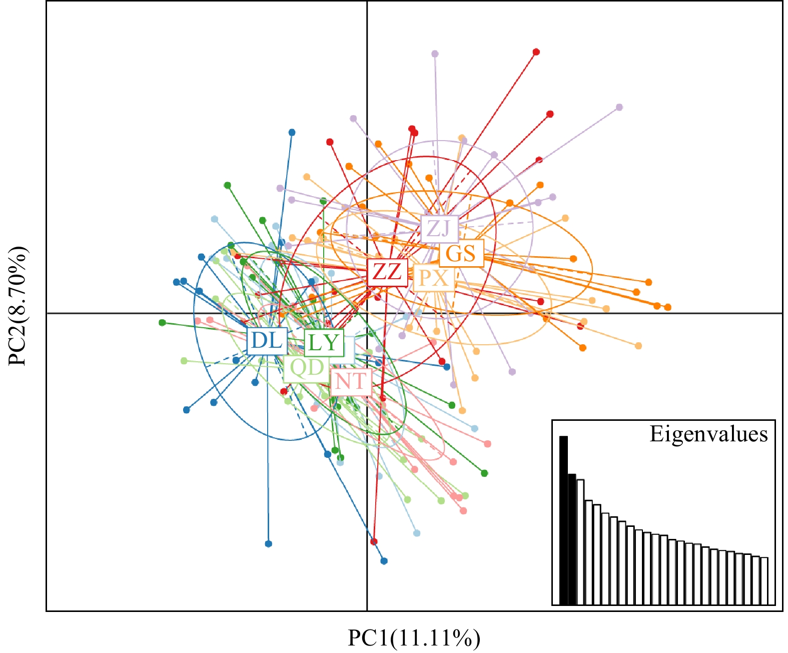
 Figure 4. Clustering result of the principal component analysis (PAC).Table 4. Analysis of molecular variance (AMOVA) of S. tenuifilis populations using microsatellites
Sources of variations df Sum of squares Variance components Percentage of variation Fixation indices Total (QH, DL, QD, LY, NT, PX, GS, ZJ) Among all populations 7 105.728 0.21106 Va3.07 FST = 0.03071 *Within populations 312 2078.400 6.66154 Vb96.93 Two groups (QH, DL, QD, LY, NT) (PX, GS, ZJ) Among groups 1 34.978 0.15458 Va2.23 FCT = 0.02226 *Among populations within group 6 70.750 0.12825 Vb1.85 FSC = 0.01889 *Within populations 312 2078.400 6.66154 Vc95.93 FST = 0.04073 *| Show TableDownLoad:
CSV
3.4 Bottleneck analysis
One-tail Wilcoxon rank tests for heterozygosity excess were not statistically significant for both TPM and SMM in each S. tenuifilis population (Table 5). Besides, the allele frequencies of all populations showed normal L-shaped distribution of the mode-shift test. Both tests indicated that all populations of S. tenuifilis did not experience demographic bottlenecks.
Table 5. Bottleneck analysis of S. tenuifilis populations under the two-phase mutation model (TPM) and stepwise mutation model (SMM)Population Wilcoxon test Mode-shift test TPM SMM One tail for
H deficiencyOne tail for
H excessOne tail for
H deficiencyOne tail for
H excessQH 0.21660 0.79813 0.10571 0.90360 normal L-shaped DL 0.01932 0.98323 0.00459 0.99619 normal L-shaped QD 0.00912 0.99225 0.00775 0.99345 normal L-shaped LY 0.37178 0.64714 0.23187 0.78340 normal L-shaped NT 0.20187 0.81227 0.14893 0.86278 normal L-shaped ZZ 0.62822 0.39098 0.44997 0.56987 normal L-shaped PX 0.03696 0.96730 0.01677 0.98550 normal L-shaped GS 0.21660 0.79813 0.09641 0.91232 normal L-shaped ZJ 0.53006 0.48998 0.31609 0.70171 normal L-shaped | Show TableDownLoad:
CSV
4. Discussion
4.1 Population genetic diversity
Overall average heterozygosity, allelic abundance and polymorphism, etc., reflects the degree of genetic variability, selection pressure and gene flow, characteristic of microsatellites derived from a greater mutation level than other genetic markers, which makes them a valuable tool for genetic diversity analyses (Arranz et al., 2001). The species considered in this study, S. tenuifilis, has relatively higher levels of genetic diversity in microsatellites (mean Na=23.25, mean Ho=0.639, mean Ra=11.625, and PIC=0.844>0.5). Compared to other Clupeiformes fishes, such as Coilia nasus (mean Na=10.65, mean Ho=0.692, and PIC=0.692) (Yang et al., 2014), Clupea pallasii (mean Na=10.50, mean Ho=0.647, and PIC=0.809) (Semenova et al., 2015), and Engraulis ringens (mean Na=11.53, mean Ho=0.590, and PIC=0.880) (Ferrada-Fuentes et al., 2018), similar high genetic diversity has also been reported. Marine fish have high genetic diversity, indicating that S. tenuifilis populations in the coastal China’s seas have a higher mutation rate and adapt to evolution. We speculate that in a short historical period, S. tenuifilisn in the coastal China’s seas will maintain a large population size and are not prone to genetic bottlenecks.
4.2 Population structure of S. tenuifilis
The genetic differentiation index (FST) is an important parameter to measure population differentiation and genetic distance (Wright, 2010). In the present study, the FST values ranged from
0.0076 to0.0515 (Table 3), and most differentiations among nine populations reached a significant level (p<0.01). Based on 16 microsatellite markers, the coastal S. tenuifilis populations in China could be divided into northern and southern groups, which was verified by STRUCTURE analysis (Fig. 3), principal component analysis (PCA) (Fig. 4), and analysis of molecular variance (AMOVA) (Table 4). Interestingly, STRUCTURE and PCA analysis supported that ZZ population showed gene mixture (Figs 3 and 4). The same results were also mentioned in a morphological study that northern and southern populations of S. tenuifilis mixed in the Changjiang River (Yangtze River) Estuary by Liu et al. (2004).This mixed phenomenon in the ZZ population and north-south differentiation of S. tenuifilis populations might result from two main factors. Firstly, historical glacial action. Some scholars have discussed that the phylogeographic pattern and genetic structure of marine fish in the coastal China’s seas are affected by the Quaternary glacial-interglacial cycle (Maggs et al., 2008; Larmuseau et al., 2009). During the glacial period, the sea level of the East China Sea, which is connected to the Bohai and Yellow Seas, dropped by about 150 m from the present, and the sea level of the South China Sea dropped by about 100-120 m, resulting in the sea level in the East China Sea is slightly lower (or in a transitional state). After the glacial period, the sea level rose and the marginal sea was reconnected. Xu (2014) reported that the northern and southern populations of S. tenuifilis had different population expansion times during the Pleistocene using mitochondrial control region sequences. Therefore, successive isolation and reconnection of marginal seas in China during the Pleistocene may have hindered gene flow between S. tenuifilis populations to some extent, promoting the divergence of genetic lineages in S. tenuifilis populations. Secondly, spatial heterogeneity. Many studies have shown that eurythermal fish living at different latitudes have undergone natural selection with spatial heterogeneity, leading to changes in population structure and heritable phenotypic differentiation, accompanied by optimized adaptations to selection pressures imposed by local environments (Han et al., 2021; Tamaki and Honza, 1991). Setipinna tenuifilis has a wide latitude distribution in the northwestern Pacific Ocean, differences in water temperature (Fig. 5a) can create different levels of selection pressure, which can affect traits related to S. tenuifilis growth and reproduction. It has been reported the southern population of S. tenuifilis in China’s coast enters the spawning period earlier than the northern population, and the asynchrony of spawning in the northern and southern populations may further limit the genetic exchange between the northern and southern populations (Zhao et al., 2016). In addition, the high flux of nutrient input from the Changjiang River Estuary to the East China Sea (Fig. 5b) has led to a high level of primary productivity (Mu et al., 2020). It may be a common feeding ground for the northern and southern S. tenuifilis populations, leading to the phenomenon of two genetic backgrounds in ZZ population.
 Figure 5. Mean sea surface temperature (a) and mean sea surface salinity (b) in the coastal region of China.
5. Conclusions
This study is the first to effectively explore the polymorphism and genetic differentiation of S. tenuifilis germplasm resources using microsatellite markers. Our results indicated that the existing high genetic diversity in S. tenuifilis may be the result of maintaining a large population size. The significant genetic structure in wild S. tenuifilis populations is consistent with previous studies, and this genetic pattern may be the natural selection of historical glacial action and spatial heterogeneity of environmental factors in the coastal China’s seas. In summary, based on the significant genetic differences of 16 microsatellite markers, it is recommended to divide the northern and southern populations of S. tenuifilis in the coastal China’s seas into two different fishery management units to develop breeding and conservation plans.
-
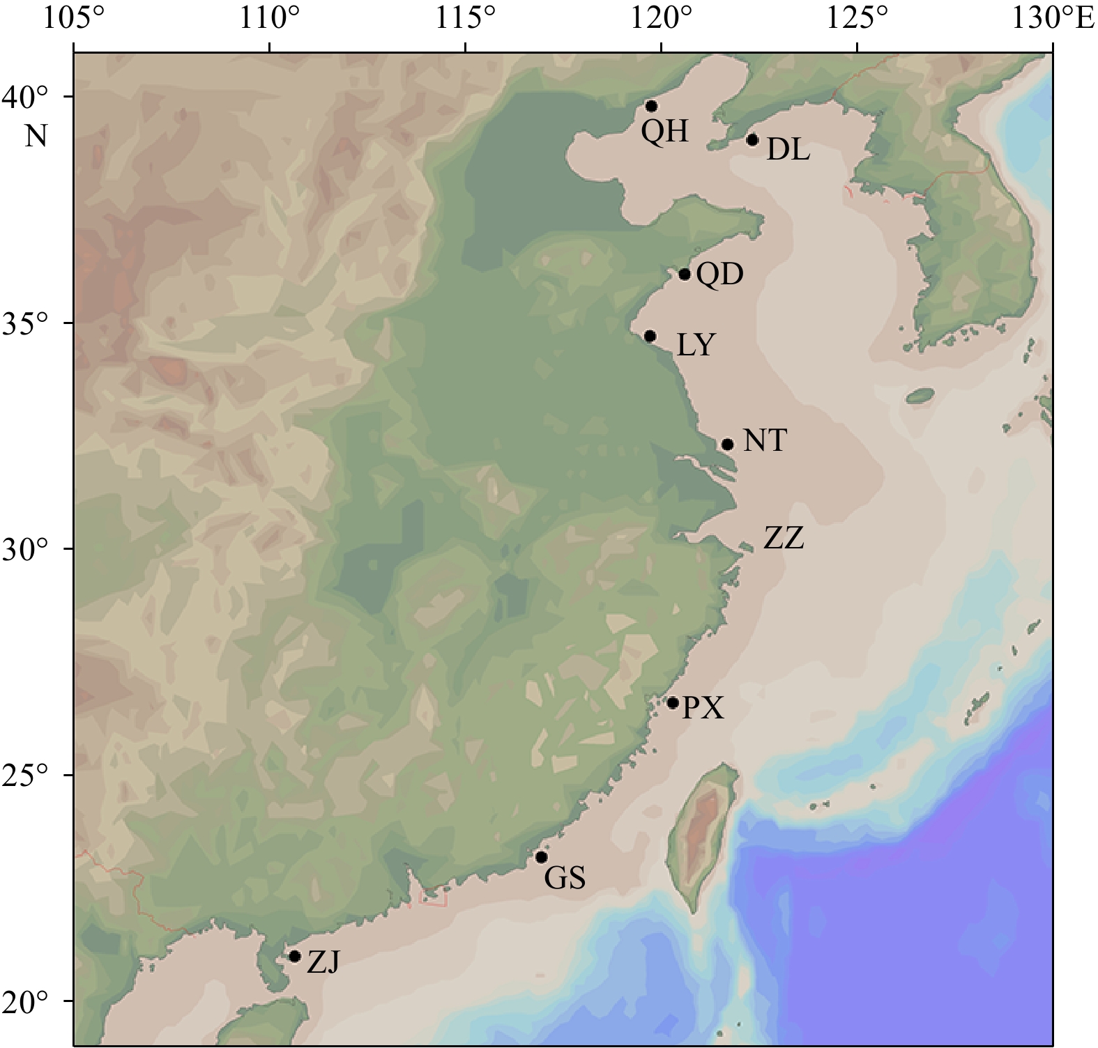
Figure 1. Schematic map of sampling locations along the coastal waters of China. A total of 180 individuals of S. tenuifilis from nine geographic locations (DL, QH, QD, LY, NT, ZZ, PX, GS, and ZJ) were collected for population analysis.
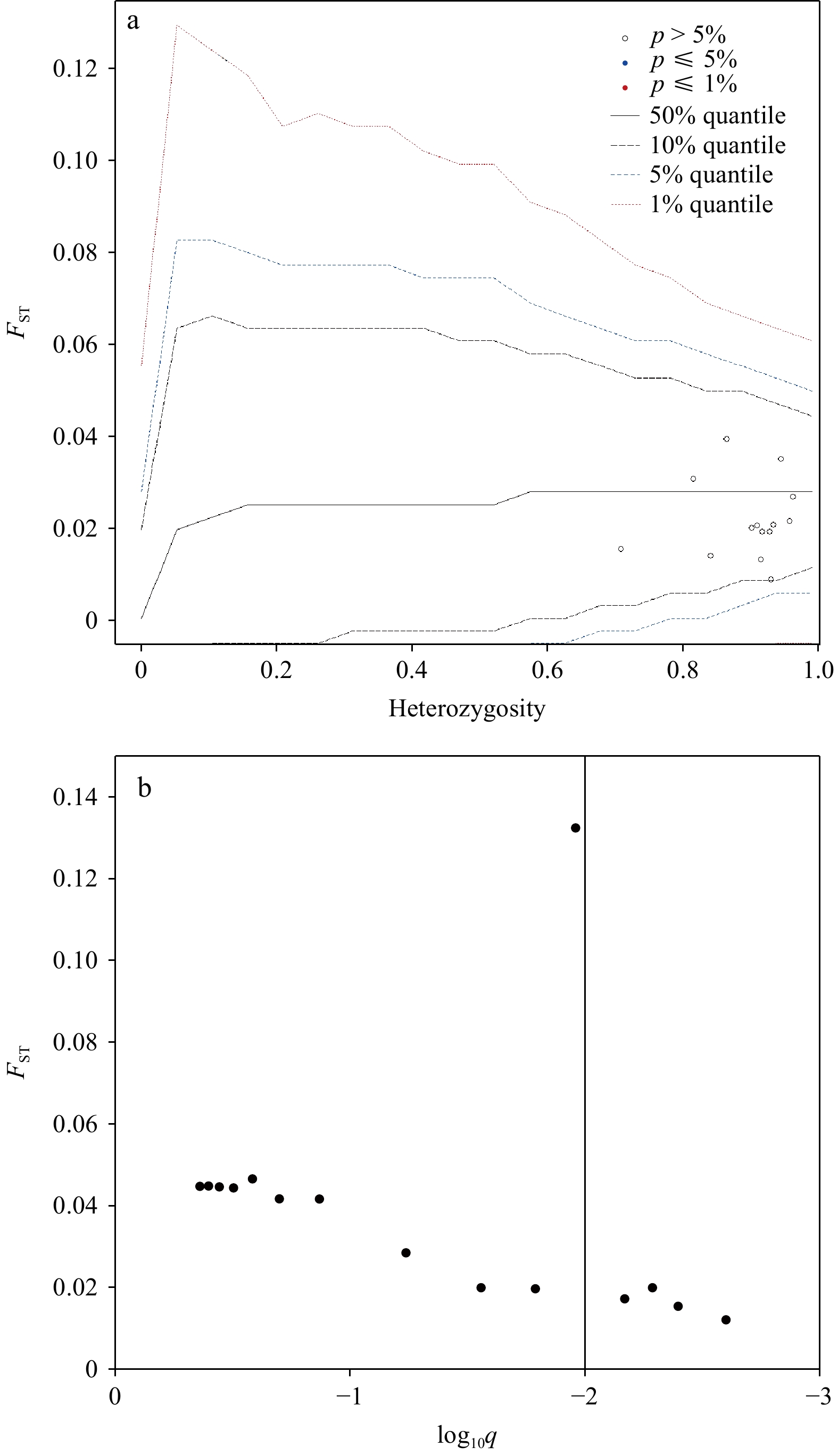
Figure 2. Plots of results of outlier tests. a. The hierarchical island model test for selection completed using the program Arlequin. The genetic differentiation (FST) is plotted against expected heterozygosity (He). b. The Bayesian test for selection completed using the program BayeScan. The dots on the right side of the vertical line are above a 0.99 probability of being candidates of selection.

Figure 3. Population structure obtained from the STRUCTURE analysis (K=2, 3, 4). Individuals are represented by vertical bars. Different colours in the same individual indicate the percentage of the genome shared with each cluster according to the admixture proportions. The Y-axis represents the probability of belonging to a certain cluster, while the X-axis represents each population delimited by a black solid vertical line.

Figure 5. Mean sea surface temperature (a) and mean sea surface salinity (b) in the coastal region of China.
Table 1. The genetic diversity of 16 polymorphic microsatellite markers for S. tenuifilis
Locus Na Ho He PIC HWE Fnull Sten01 20 0.794 0.869 0.899 NS 0.0664 Sten02 31 0.750 0.899 0.923 *** 0.1080 Sten03 21 0.756 0.887 0.918 *** 0.1013 Sten04 32 0.572 0.914 0.951 *** 0.2498 Sten05 17 0.867 0.861 0.887 NS 0.0163 Sten06 18 0.394 0.680 0.677 *** 0.2921 Sten07 27 0.611 0.770 0.792 *** 0.1190 Sten08 22 0.544 0.877 0.906 *** 0.2517 Sten09 45 0.467 0.914 0.956 *** 0.3455 Sten10 28 0.450 0.889 0.936 *** 0.3531 Sten11 17 0.700 0.808 0.818 *** 0.0879 Sten12 21 0.817 0.880 0.904 NS 0.0551 Sten13 12 0.572 0.668 0.714 *** 0.1288 Sten14 17 0.606 0.809 0.845 *** 0.1739 Sten15 29 0.911 0.892 0.925 NS 0.0086 Sten16 15 0.411 0.418 0.445 NS 0.0645 Mean 23.25 0.639 0.815 0.844 0.1514 Notes: Na represents number of alleles, Ho observed heterozygosity, He expected heterozygosity, PIC polymorphic information content, HWE deviation from the Hardy-Weinberg equilibrium (NS meaning non-significant and *** less than 0.0001 ), and Fnull null allele frequency. 下载: 导出CSV
Table 2. Genetic diversity of nine S. tenuifilis populations
Population Ra Na Ho He QH 12.125 12.125 0.616 0.805 DL 11.688 11.688 0.578 0.787 QD 12.188 12.188 0.638 0.798 LY 11.813 11.813 0.659 0.814 NT 11.688 11.688 0.625 0.805 ZZ 11.188 11.188 0.625 0.838 PX 11.188 11.188 0.663 0.816 GS 10.938 10.938 0.678 0.822 ZJ 11.813 11.813 0.669 0.847 Mean 11.625 11.625 0.639 0.815 Notes: Ra represents allelic richness, Na number of alleles, Ho observed heterozygosity, and He expected heterozygosity.
下载: 导出CSV
Table 3. Pairwise genetic differentiation (FST) for nine S. tenuifilis populations using microsatellites
QH DL QD LY NT ZZ PX GS ZJ QH DL 0.0327 QD 0.0240 0.0229 LY 0.0190 0.0265 0.0174 NT 0.0120 0.0295 0.0147 0.0198 ZZ 0.0158 0.0345 0.0249 0.0249 0.0182 PX 0.0370 0.0504 0.0381 0.0312 0.0281 0.0220 GS 0.0373 0.0515 0.0443 0.0364 0.0329 0.0165 0.0076 ZJ 0.0368 0.0479 0.0466 0.0366 0.0423 0.0115 0.0227 0.0093 Notes: Extremely significant difference probability values (p<0.01) following correction for multiple tests are indicated in bold.
下载: 导出CSV
Table 4. Analysis of molecular variance (AMOVA) of S. tenuifilis populations using microsatellites
Sources of variations df Sum of squares Variance components Percentage of variation Fixation indices Total (QH, DL, QD, LY, NT, PX, GS, ZJ) Among all populations 7 105.728 0.21106 Va3.07 FST = 0.03071 *Within populations 312 2078.400 6.66154 Vb96.93 Two groups (QH, DL, QD, LY, NT) (PX, GS, ZJ) Among groups 1 34.978 0.15458 Va2.23 FCT = 0.02226 *Among populations within group 6 70.750 0.12825 Vb1.85 FSC = 0.01889 *Within populations 312 2078.400 6.66154 Vc95.93 FST = 0.04073 *
下载: 导出CSV
Table 5. Bottleneck analysis of S. tenuifilis populations under the two-phase mutation model (TPM) and stepwise mutation model (SMM)
Population Wilcoxon test Mode-shift test TPM SMM One tail for
H deficiencyOne tail for
H excessOne tail for
H deficiencyOne tail for
H excessQH 0.21660 0.79813 0.10571 0.90360 normal L-shaped DL 0.01932 0.98323 0.00459 0.99619 normal L-shaped QD 0.00912 0.99225 0.00775 0.99345 normal L-shaped LY 0.37178 0.64714 0.23187 0.78340 normal L-shaped NT 0.20187 0.81227 0.14893 0.86278 normal L-shaped ZZ 0.62822 0.39098 0.44997 0.56987 normal L-shaped PX 0.03696 0.96730 0.01677 0.98550 normal L-shaped GS 0.21660 0.79813 0.09641 0.91232 normal L-shaped ZJ 0.53006 0.48998 0.31609 0.70171 normal L-shaped
下载: 导出CSV
-
Arranz J J, Bayón Y, San Primitivo F. 2001. Genetic variation at microsatellite loci in Spanish sheep. Small Ruminant Research, 39(1): 3–10, doi: 10.1016/s0921-4488(00)00164-4 Beaumont M A. 2008. Selection and sticklebacks. Molecular Ecology, 17(15): 3425–3427, doi: 10.1111/j.1365-294x.2008.03863.x Beaumont M A, Balding D J. 2004. Identifying adaptive genetic divergence among populations from genome scans. Molecular Ecology, 13(4): 969–980, doi: 10.1111/j.1365-294x.2004.02125.x Cornuet J M, Luikart G. 1996. Description and power analysis of two tests for detecting recent population bottlenecks from allele frequency data. Genetics, 144(4): 2001–2014, doi: 10.1093/genetics/144.4.2001 Earl D A, VonHoldt B M. 2012. STRUCTURE HARVESTER: a website and program for visualizing STRUCTURE output and implementing the Evanno method. Conservation Genetics Resources, 4(2): 359–361, doi: 10.1007/s12686-011-9548-7 Evanno G, Regnaut S, Goudet J. 2005. Detecting the number of clusters of individuals using the software STRUCTURE: a simulation study. Molecular Ecology, 14(8): 2611–2620., doi: 10.1111/j.1365-294X.2005.02553.x Excoffier L, Hofer T, Foll M. 2009. Detecting loci under selection in a hierarchically structured population. Heredity, 103(4): 285–298, doi: 10.1038/hdy.2009.74 Excoffier L, Lischer H E L. 2010. Arlequin suite ver 3.5: a new series of programs to perform population genetics analyses under Linux and Windows. Molecular Ecology Resources, 10(3): 564–567, doi: 10.1111/j.1755-0998.2010.02847.x Ferrada-Fuentes S, Galleguillos R, Canales-Aguirre C B, et al. 2018. Development and characterization of thirty-two microsatellite markers for the anchovy, Engraulis ringens Jenyns, 1842 (Clupeiformes, Engraulidae) via 454 pyrosequencing. Latin American Journal of Aquatic Research, 46(2): 452–456, doi: 10.3856/vol46-issue2-fulltext-19 Foll M, Gaggiotti O. 2008. A genome-scan method to identify selected loci appropriate for both dominant and codominant markers: a Bayesian perspective. Genetics, 180(2): 977–993, doi: 10.1534/genetics.108.092221 Goudet J. 2001. FSTAT, a program to estimate and test gene diversities and fixation (version 2.9. 3.2). https://www.scienceopen.com/document?vid=188bd209-47c8-4e90-8a28-4f744b22cf85[2011-06-18/2023-11-01] Han Zhiqiang, Guo Xinyu, Liu Qun, et al. 2021. Whole-genome resequencing of Japanese whiting (Sillago japonica) provide insights into local adaptations. Zoological Research, 42(5): 548–561, doi: 10.24272/j.issn.2095-8137.2021.116 Hedrick P W. 2005. A standardized genetic differentiation measure. Evolution, 59(8): 1633–1638, doi: 10.1554/05-076.1 Hulce D, Li X, Snyder-Leiby T, et al. 2011. GeneMarker® genotyping software: Tools to increase the statistical power of DNA fragment analysis. Journal of Biomolecular Techniques, 22(S): S35–S36 Jakobsson M, Rosenberg N A. 2007. CLUMPP: a cluster matching and permutation program for dealing with label switching and multimodality in analysis of population structure. Bioinformatics, 23(14): 1801–1806, doi: 10.1093/bioinformatics/btm233 Kalinowski S T, Taper M L, Marshall T C. 2007. Revising how the computer program CERVUS accommodates genotyping error increases success in paternity assignment. Molecular Ecology, 16(5): 1099–1106, doi: 10.1111/j.1365-294X.2007.03089.x Larmuseau M H D, Van Houdt J K J, Guelinckx J, et al. 2009. Distributional and demographic consequences of Pleistocene climate fluctuations for a marine demersal fish in the north-eastern Atlantic. Journal of Biogeography, 36(6): 1138–1151, doi: 10.1111/j.1365-2699.2008.02072.x Li Jiasheng, Liu Bingjian, Chen Shiyi, et al. 2022. Development and characterization of seventeen novel microsatellite markers in common hairfin anchovy (Setipinna tenuifilis) using third-generation sequencing technology. Journal of Applied Ichthyology, 38(4): 462–467, doi: 10.1111/jai.14335 Liu Yong, Cheng Jiahua, Li Shengfa. 2004. A study on the distribution of Setipinna taty in the East China Sea. Marine Fisheries (in Chinese), 26(4): 255–260, doi: 10.3969/j.issn.1004-2490.2004.04.002 Liu Bingjian, Li Jiasheng, Peng Ying, et al. 2024. Chromosome-level genome assembly and population genomic analysis reveal evolution and local adaptation in common hairfin anchovy (Setipinna tenuifilis). Molecular Ecology, 33(10): e17067, doi: 10.1111/mec.17067 Maggs C A, Castilho R, Foltz D, et al. 2008. Evaluating signatures of glacial refugia for North Atlantic benthic marine taxa. Ecology, 89(sp11): S108–S122, doi: 10.1890/08-0257.1 Mu Jinglong, Zhang Shanshan, Liang Cui, et al. 2020. Temporal and spatial distribution and mixing behavior of nutrients in the Changjiang River Estuary. Marine Sciences (in Chinese), 44(1): 19–35 Narum S R, Hess J E. 2011. Comparison of FST outlier tests for SNP loci under selection. Molecular Ecology Resources, 11(s1): 184–194, doi: 10.1111/j.1755-0998.2011.02987.x Peakall R O D, Smouse P E. 2006. GENALEX 6: genetic analysis in Excel. Population genetic software for teaching and research. Molecular Ecology Notes, 6(1): 288–295, doi: 10.1111/j.1471-8286.2005.01155.x Piry S, Luikart G, Cornuet J M. 1999. Computer note. BOTTLENECK: a computer program for detecting recent reductions in the effective size using allele frequency data. Journal of Heredity, 90(4): 502–503, doi: 10.1093/jhered/90.4.502 Pritchard J K, Stephens M, Donnelly P. 2000. Inference of population structure using multilocus genotype data. Genetics, 155(2): 945–959, doi: 10.1093/genetics/155.2.945 Rosenberg N A. 2004. DISTRUCT: a program for the graphical display of population structure. Molecular Ecology Notes, 4(1): 137–138, doi: 10.1046/j.1471-8286.2003.00566.x Rousset F. 2008. genepop’007: a complete re-implementation of the genepop software for Windows and Linux. Molecular Ecology Resources, 8(1): 103–106, doi: 10.1111/j.1471-8286.2007.01931.x Semenova A V, Stroganov A N, Afanasiev K I, et al. 2015. Population structure and variability of Pacific herring (Clupea pallasii) in the White Sea, Barents and Kara Seas revealed by microsatellite DNA analyses. Polar Biology, 38(7): 951–965, doi: 10.1007/s00300-015-1653-8 Sheng Yan, Zheng Weihong, Pei Kequan, et al. 2002. Applications of microsatellites in population biology. Acta Plytoecologica Sinica (in Chinese), 26(S1): 119–126 Song Na, Yin Lina, Sun Dianrong, et al. 2019. Fine-scale population structure of Collichtys lucidus populations inferred from microsatellite markers. Journal of Applied Ichthyology, 35(3): 709–718, doi: 10.1111/jai.13902 Tamaki K, Honza E. 1991. Global tectionics and formation of marginal basins: role of the western Pacific. Episodes Journal of International Geoscience, 14(3): 224–230, doi: 10.18814/EPIIUGS/1991/V14I3/005 Vicente A A, Carolino M I, Sousa M C O, et al. 2008. Genetic diversity in native and commercial breeds of pigs in Portugal assessed by microsatellites. Journal of Animal Science, 86(10): 2496–2507, doi: 10.2527/jas.2007-0691 Wachowiak W, Balk P A, Savolainen O. 2009. Search for nucleotide diversity patterns of local adaptation in dehydrins and other cold-related candidate genes in Scots pine (Pinus sylvestris L.). Tree Genetics & Genomes, 5(1): 117–132, doi: 10.1007/s11295-008-0188-3 Wang Wei, Ma Chunyan, Ouyang Longling, et al. 2021. Genetic diversity and population structure analysis of Lateolabrax maculatus from Chinese coastal waters using polymorphic microsatellite markers. Scientific Reports, 11(1): 15260, doi: 10.1038/s41598-021-93000-6 Wright S. 2010. Variability Within and Among Natural Populations. Illinois: University of Chicago Press (查阅网上资料, 未找到出版地信息, 请确认) Xu Shengyong. 2014. Morphology and genetics of Setipinna tenuifilis (in Chinese)[dissertation]. Qingdao: Ocean University of China Xu Shengyong, Song Na, Lu Zhichuang, et al. 2014. Genetic variation in scaly hair-fin anchovy Setipinna tenuifilis (Engraulididae) based on the mitochondrial DNA control region. Mitochondrial DNA, 25(3): 223–230, doi: 10.3109/19401736.2013.845754 Yang Qiaoli, Gao Tianxiang, Liu Jinxian. 2014. Development and characterization of 17 microsatellite loci in an anadromous fish Coilia nasus. Conservation Genetics Resources, 6(2): 357–359, doi: 10.1007/s12686-013-0093-4 Zhang Bo. 2013. Molecular marker development and genetic diversity analysis of Setipinna tenuifilis (in Chinese) [dissertation]. Zhoushan: Zhejiang Ocean University Zhao Shenglong, Xu Hanxiang, Zhong Junsheng, et al. 2016. Zhejiang Marine Fish Records (in Chinese). Hangzhou: Zhejiang Science and Technology Press Zuccaro A, Bordonaro S, Criscione A, et al. 2008. Genetic diversity and admixture analysis of Sanfratellano and three other Italian horse breeds assessed by microsatellite markers. Animal, 2(7): 991–998, doi: 10.1017/S1751731108002255 -

 DownLoad:
 点击查看大图
计量
- 文章访问数: 43
- HTML全文浏览量: 17
- 被引次数: 0

