

Effects of hypoxia on community structure of macrobenthos in the Pearl River Estuary
-
Abstract: Macrobenthos can serve as an indicator of hypoxia in the estuarine ecosystem. This comparative study surveyed macrobenthos from hypoxic and non-hypoxic areas of the Pearl River Estuary (PRE), and explores the effects of environmental factor on the macrobenthos community structure. In July 2020, 49 macrobenthos species were collected from the hypoxic area, contrasting with 91 species found in the non-hypoxic area. July 2021 recorded 51 species in the hypoxic area and 76 in the non-hypoxic area. Analysis of Similarities (ANOSIM) and Non-metric Multidimentional Scaling (NMDS) showed no significant difference in the macrobenthos community structure between the two areas. However, Polychaeta displays higher species richness, abundance, and biomass in the hypoxic zone, negatively correlating correlation to dissolved oxygen (DO). Canonical Correspondence Analysis (CCA) also showed that the abundance of Polychaeta was negatively correlated with that of Crustacea. Interestingly, despite the differences in Polychaeta, macrobenthos community structure remains stable between hypoxic and non-hypoxic samples. This study suggests Polychaeta's potential adaptation to hypoxic conditions in the PRE's hypoxic area. Finally, Spearman correlation analysis showed that DO have a significant negative correlation with total phosphorus (TP), total nitrogen (TN) and total organic carbon (TOC) in the PRE, indicating that water eutrophication would exacerbate the occurrence of hypoxia.
-
Key words:
- hypoxia /
- macrobenthos /
- community structure /
- Pearl River Estuary
-
1. Introduction
The South China Sea (SCS) is a semi-enclosed marginal sea of the North Pacific Ocean. It extends from the equator to 23°N and from 99°E to 121°E, with an average water depth of over 2 000 m and the maximum depth of approximately 4 700 m (Chu and Li, 2000). The SCS connects the adjacent seas through the Taiwan, Luzon Strait, Mindoro, Balabac, Karimata and Malacca Straits. The Luzon Strait is the only deep strait with a sill depth of about 2 400 m, and it plays a major role in the water exchange between the SCS and the Pacific Ocean (Qu et al., 2006; Deng et al., 2018; Wu et al., 2021).
The annual mean Luzon Strait transport is westward, with transport ranging from 2×10⁶ m3/s to 10×106 m3/s (Metzger and Hurlburt, 1996; Xue et al., 2004; Fang et al., 2005, 2009; Yaremchuk et al., 2009; Hsin et al., 2012). Its sandwiched vertical structure has been proposed based on historical oxygen data and current observations (Qu, 2002; Tian et al., 2006). Through the Luzon Strait, water flows into the SCS in the upper and deep layers but flows out of the SCS in the intermediate layer. The Luzon Strait transport has a distinct seasonal variation, with stronger transport in winter and weaker transport in summer (Qu, 2000; Fang et al., 2005; Yaremchuk et al., 2009; Zhang et al., 2015). This seasonal variation is attributed to the seasonal reversal of the SCS monsoon (Metzger and Hurlburt, 1996; Zhao et al., 2009; Hsin et al., 2012), as well as the influence of the Kuroshio transport east of Luzon (Qu et al., 2004; Yaremchuk and Qu, 2004; Yang et al., 2013).
The Luzon Strait transport has important impacts on the SCS circulation. The upper layer circulation in the SCS is mainly driven by the SCS monsoon (Yang et al., 2002; Xue et al., 2004; Gan et al., 2006), but the Kuroshio intrusion through the Luzon Strait and mesoscale eddies that shed from Kuroshio near the Luzon Strait impose an important influence on the circulation pattern in the northern SCS (Xue et al., 2004; Nan et al., 2011, 2015; Zhang et al., 2017). In the meantime, the Luzon Strait upper layer inflow can enhance upper layer cyclonic circulation in the SCS (Chen and Xue, 2014; Xu and Oey, 2014; Li et al., 2019). The major feature of the SCS intermediate layer circulation is anticyclonic (Yuan, 2002; Shu et al., 2014; Xu and Oey, 2014), and Zhu et al. (2017) suggested that the negative potential vorticity transport caused by the Luzon Strait intermediate layer outflow is responsible for the anticyclonic circulation formation. There is a cyclonic circulation in the SCS deep layer (Qu et al., 2006; Wang et al., 2011), since the persistent deepwater overflow through the Luzon Strait provides a positive potential vorticity transport for the deep SCS and makes water move cyclonically (Lan et al., 2013). The Luzon Strait transport influences the SCS water properties (Qu et al., 2000; Wei et al., 2016) and balances the heat and salt budgets of the SCS (Qu et al., 2004; Yu et al., 2008; Fang et al., 2009). It contributes to extreme subsurface warm events in the SCS (Xiao et al., 2018) and plays an important role in long-term variabilities of salinity in the surface and subsurface layers (Zeng et al., 2016, 2021).
The shallow meridional overturning circulation (SMOC) in the upper SCS is clockwise on annual mean (Shu et al., 2014; Zhang et al., 2016), and it is essential for the vertical link between the surface layer and the subsurface layer. The SMOC has a prominent seasonal variation, with a clockwise structure in winter and an anticlockwise structure in summer (Jiang et al., 2023). The structure of the SMOC is shown by stream functions, and stream functions are under the influences of the Luzon Strait transport (Wang et al., 2004). Hence, the Luzon Strait transport may have an important influence on the SMOC. Some studies paid attention to the connection between the Luzon Strait transport and the SMOC in the SCS. Numerical experiments are carried out with the Luzon Strait open and closed in Wang et al. (2004), and their results suggested that the impact extent of the Luzon Strait transport on the upper layer stream function can reach 10°N. The SMOC can still be formed in the numerical experiment with the Luzon Strait closed, indicating that the SMOC formation is not dominated by the Luzon Strait transport. Shu et al. (2014) calculated the Lagrangian stream function to illustrate the contribution of Luzon Strait transport to the SMOC. In their results, the Lagrangian stream functions which show the SMOC structure are mainly caused by the Luzon Strait transport, suggesting that the Luzon Strait transport dominates the SMOC formation. Wang et al. (2004) and Shu et al. (2014) both pointed out that the Luzon Strait transport has an influence on the SMOC in the SCS, but they have differences on the issue whether the Luzon Strait transport dominates the SMOC formation. So far, this issue remains a matter of controversy, and there are no other studies discussing it.
In the present study, the aim is to investigate whether the Luzon Strait transport dominates the SMOC formation. The Helmholtz decomposition has been applied into the Indian Ocean to separate the Indonesian Throughflow (ITF) and the Antarctic Circumpolar Current (ACC) from the total zonally integrated flow (Han and Huang, 2020), and we apply this method into the SCS. The rest of the study is structured as follows. The data and Helmholtz decomposition method are introduced in section 2. The Helmholtz decomposition results in winter (December) and summer (June) are presented in section 3. Section 4 is some discussion based on numerical experiments. The summary of this study is given in section 5.
2. Data and method
The Ocean General Circulation Model for the Earth Simulator (OFES) products from 1985 to 2005 are used in this study. The OFES is based on the Modular Ocean Model (MOM3) and developed at Geophysical Fluid Dynamics Laboratory/National Oceanic and Atmospheric Administration (GFDL/NOAA). OFES has a computational domain ranging from 75°S to 75°N. Its horizontal resolution is 0.1°, and there are 54 levels in vertical direction. The vertical mixing is calculated by the K-Profile Parameterization scheme. Monthly mean wind stresses that used for the climatological seasonal integration are from the National Centers for Environmental Prediction/National Center for Atmospheric Research (NCEP/NCAR) reanalysis data. More information of OFES is available in Masumoto et al. (2004) and Sasaki et al. (2008).
The Helmholtz decomposition is used to separate the motion caused by the Luzon Strait transport from total zonally integrated flow in the SCS. According to Han and Huang (2020), zonally integrating the continuity equation leads to
$$ \frac{\partial V}{\partial y}+\frac{\partial W}{\partial z}={u}_{\mathrm{w}}-{u}_{\mathrm{e}} {\mathrm{,}}\; $$ (1) where
$$ V={\int }_{{x}_{\mathrm{w}}}^{{x}_{\mathrm{e}}}vdx {\mathrm{,}}\; W={\int }_{{x}_{\mathrm{w}}}^{{x}_{\mathrm{e}}}wdx {\mathrm{,}}\; $$ (2) in which
$ V $ and$ W $ denote the total zonally integrated meridional velocity and vertical velocity, respectively.$ {u}_{\mathrm{e}} $ and$ {u}_{\mathrm{w}} $ are the zonal velocities at the eastern and western boundaries of the SCS,$ {x}_{\mathrm{e}} $ and$ {x}_{\mathrm{w}} $ are the eastern and western boundaries of the SCS basin, and$ v $ and$ w $ are the meridional and vertical velocity components. The right term in Eq. (1) is the divergence term. The western boundary of the SCS is the Asian landmass, and the divergence term is caused by the zonal velocities in straits at the eastern boundary. Water enters the SCS in the southern part of the Luzon Strait and leaves the SCS in the northern part (Fig. 1). Water also flows out of the SCS through the Mindoro Strait near 13°N (Fig. 1; Fang et al., 2009; Yaremchuk et al., 2009). The water exchange through the Balabac Strait near 8°N is weak. The Luzon Strait transport makes the largest contribution to the nonzero divergence term. Figure 1. Zonal velocities (m/s, eastward positive) at the eastern boundary of the SCS in winter (a) and summer (b).
In the Helmholtz decomposition,
$ V $ and$ W $ are decomposed as$$ V={V}_{\Psi }+{V}_{\Phi } {\mathrm{,}}\; W={W}_{\Psi }+{W}_{\Phi } {\mathrm{,}}\; $$ (3) where
$ {V}_{\Psi } $ and$ {W}_{\Psi } $ are the rotational components of$ V $ and$ W $ , and$ {V}_{\Phi } $ and$ {W}_{\Phi } $ are the divergent components. Definitions of the rotational components and the divergent components are$$ {V}_{\Psi }=-\frac{\partial \Psi }{\partial z} {\mathrm{,}}\; {V}_{\Phi }=\frac{\partial \Phi }{\partial y} {\mathrm{,}}\; $$ (4) $$ {W}_{\Psi }=\frac{\partial \Psi }{\partial y} {\mathrm{,}}\; {W}_{\Phi }=\frac{\partial \Phi }{\partial z} {\mathrm{,}}\; $$ (5) where
$ \Psi $ denotes the stream function, and$ \Phi $ denotes the potential function. Substituting Eqs. (3)‒(5) into Eq. (1) leads to a Poisson equation,$$ \frac{{\partial }^{2}\Phi }{\partial {y}^{2}}+\frac{{\partial }^{2}\Phi }{\partial {z}^{2}}={u}_{w}-{u}_{e} . $$ (6) According to Eq. (6), the divergence term is indicated by the potential function
$ {\Phi } $ . Hence, solving the Poisson equation can obtain the potential function and divergent components, and then separate the motion in the SCS caused by the Luzon Strait transport.Boundary conditions are given to solve the Poisson equation. Following Han and Huang (2020), the normal velocity caused by the potential function
$ \Phi $ at the bottom boundary is zero, which leads to the bottom boundary condition$$ \frac{\partial \Phi }{\partial n}=0 {\mathrm{,}}\; {\mathrm{at\; sea\; bottom}} {\mathrm{,}}\; $$ (7) where
$ n $ is the normal unit vector at sea bottom. For the OFES products, in winter, the outward transports through the Taiwan, Mindoro, Balabac and Karimata Straits are 0.77 × 10⁶ m3/s, 2.98 × 10⁶ m3/s, 0.60 × 10⁶ m3/s, and 2.56 × 10⁶ m3/s, respectively. The outward transports, amounting to 6.91 × 10⁶ m3/s, are basically balanced by the inward transport of 6.87 × 10⁶ m3/s through the Luzon Strait with a residual of 0.04 × 10⁶ m3/s. In summer, the outward transports through the Taiwan, Mindoro and Balabac Straits are 1.78 × 10⁶ m3/s, 0.96 × 10⁶ m3/s, and 0.13 × 10⁶ m3/s, respectively. The inward transports through the Luzon and Karimata Straits are 2.18 × 10⁶ m3/s and 0.69 × 10⁶ m3/s. The outward transports (2.87 × 10⁶ m3/s) are balanced by the inward transports (2.87 × 10⁶ m3/s). Thus, the neglection of the volume flux at the sea surface is an acceptable approximation, and the surface boundary condition is taken as$$ \frac{\partial \Phi }{\partial z}=0 {\mathrm{,}}\; {\mathrm{at\; sea\; surface}}. $$ (8) The Poisson equation (Eq. (6)) is solved numerically using the ‘‘successive over-relaxation iteration’’ (SOR) method incorporating the surface and bottom boundary conditions (Eqs. (7) and (8)). More information of the SOR method is available in Han and Huang (2020). The Karimata Strait and the Taiwan Strait are located at the southern and northern boundaries of the SCS, respectively. The two straits are important for the mass balance of the SCS although their depths are shallow. In this study, the two straits are open in the process of solving the Poisson equation, and the flows caused by the potential function can enter or leave the SCS through them.
Two numerical experiments used in this study are designed on the basis of the Hybrid Coordinate Ocean Model (HYCOM; Bleck, 2002). The HYCOM has been used to explore the SCS circulation (Lan et al., 2013; Zhao et al., 2020), and their results have illustrated the reliability of the HYCOM in simulating the SCS circulation. The model domain is from 78°S to 66°N with a horizontal resolution of 0.5°×0.5°cos
$ \theta $ ($ \theta $ denotes latitude), and there are 33 levels in the vertical direction. The ETOPO5 is used to construct the model bottom topography. The surface forcings are from the monthly NCEP/NCAR reanalysis data, including wind forcing, the net shortwave and longwave radiation, precipitation, air relative humidity, and air temperature fields. The model is integrated for 50 years with zero initial velocities and with temperature and salinity from Levitus annual mean climatology (Levitus, 1983). The Luzon Strait is open in the control run, and closed in the sensitivity run.3. The Helmholtz decomposition results
The curls of the decomposed divergent components and the divergences of the decomposed rotational components are basically zero, indicating the validity of our Helmholtz decomposition results. The SMOC in the SCS is depicted by the stream functions, which are calculated by vertically integrating
$ V $ and$ {V}_{\Psi } $ from sea surface to sea bottom and are denoted as$ \psi \left(V\right) $ and$ \psi \left({V}_{\Psi }\right) $ , respectively. Along a stream function isoline, water moves clockwise around the higher value. Patterns of$ \psi \left(V\right) $ and$ \psi \left({V}_{\Psi }\right) $ in winter and summer are shown in Fig. 2 to illustrate the influence of the Luzon Strait transport on the stream functions. Figure 2. Stream functions (106 m3/s) obtained by vertically integrating the total zonally integrated meridional velocity
$ V $ (a) and the rotational component$ {V}_{\Psi } $ (b) in winter. (c) and (d) are same as (a) and (b), but in summer.In winter, it is evident that the
$ \psi \left(V\right) $ pattern exhibits a clockwise SMOC spanning a 9–18°N latitude range (Fig. 2a). It consists of the water sinking in the northern SCS, the water rising in the southern SCS, the northward surface transport and the southward subsurface transport. After the motion generated by the Luzon Strait transport being removed, the clockwise SMOC between 9°N and 18°N is still shown clearly in the$ \psi \left({V}_{\Psi }\right) $ pattern (Fig. 2b). The similarity between the$ \psi \left(V\right) $ pattern and the$ \psi \left({V}_{\Psi }\right) $ pattern indicates that the Luzon Strait transport has no significant influence on the SMOC structure in winter.In summer, the
$ \psi \left(V\right) $ pattern presents an anticlockwise SMOC in the southern SCS, with an upwelling branch near 12°N, a downwelling branch near 6°N, a southward surface branch and a northward subsurface branch (Fig. 2c). When the motion caused by the Luzon Strait transport is removed, the$ \psi \left({V}_{\Psi }\right) $ pattern closely resembles the$ \psi \left(V\right) $ pattern, and an anticlockwise summer SMOC is still maintained in the southern SCS (Fig. 2d). Hence, the Luzon Strait transport imparts little influence on the SMOC structure in summer.The divergent component
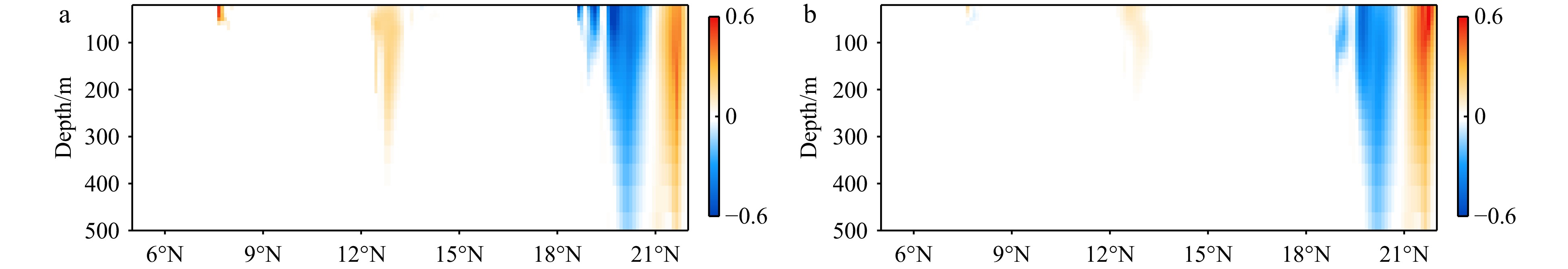
$ {V}_{\Phi } $ that separated from total zonally integrated meridional velocity is shown in Fig. 3, reflecting features of the motion that caused by the Luzon Strait transport. The Luzon Strait transport is inward to the SCS from the Pacific Ocean and the Mindoro Strait (near 13°N, south of the Luzon Strait) transport is outward to the Sulu Sea (Fang et al., 2009; Yaremchuk et al., 2009), and thus, the divergent component$ {V}_{\Phi } $ in the upper 100 m depicts a distinct southward flow extending from 20°N to 13°N (Fig. 3). This southward flow has higher intensity in winter and lower intensity in summer, also corresponding to the prominent seasonal variation of the Luzon Strait upper layer transport which is stronger in winter and weaker in summer (Qu, 2000; Zhang et al., 2015). This southward flow makes differences between the$ \psi \left(V\right) $ pattern and the$ \psi \left({V}_{\Psi }\right) $ pattern north of 13°N more significant in winter (Fig. 2). The Luzon Strait transport also causes flows south of 13°N, but intensities of these flows are weaker than that north of 13°N (Fig. 3). As a result, differences between the$ \psi \left(V\right) $ pattern and the$ \psi \left({V}_{\Psi }\right) $ pattern south of 13°N are less obvious than that north of 13°N (Fig. 2). In general, the Helmholtz decomposition results suggest that the Luzon Strait transport does not dominate the formation and seasonal variation of the SMOC although it imposes some influence on the upper layer stream functions, which is consistent with the results in Wang et al. (2004). Figure 3. The divergent component
$ {V}_{\Phi } $ (104 m2/s, northward positive) of total zonally integrated meridional velocity in winter (a) and summer (b).4. Discussion
Two numerical experiments are conducted to further confirm the conclusion in section 3. The Luzon Strait is open in the control run and closed in the sensitivity run. The two numerical experiments in this study use the SCS topography and keep the Taiwan, Mindoro, and Karimata Straits open. Our numerical experiments are improved when compared with the numerical experiments in Wang et al. (2004) which have a flat bottom (1 000 m) and treat most straits as an enclose boundary excluding the Luzon Strait.
We validate the surface circulations from the control run using the horizontal velocities of Ocean Surface Currents Analyses Real-time version 2.0 (OSCARv2.0) products from 1993 to 2020 which are calculated from sea surface height, surface wind and sea surface temperature that collected from satellites and in situ measurements (Bonjean and Lagerloef, 2002). The surface circulations from control run and OSCARv2.0 products are shown in Fig. 4. In winter, water enters into the South China Sea (SCS) through the Luzon Strait, and there is a basin scale cyclonic gyre in the SCS (Figs. 4a and c). In summer, the Kuroshio leaps across the Luzon Strait, and an anticyclonic gyre occurs in the southern SCS (Figs. 4b and d). The surface circulation patterns near the Luzon Strait and within the SCS from the control run results are consistent with those from observations. Besides, in the control run result, the Luzon Strait transport above 100 m is westward in winter with a strength of 2.45 × 10⁶ m3/s, while it is eastward in summer with a strength of 1.46 × 10⁶ m3/s, which is consistent with previous studies (Fang et al., 2009; Zhu et al., 2016). Overall, the control run is capable of simulating the Luzon Strait transport and the SCS circulations.
 Figure 4. Surface circulation (in m/s) in winter (a) and summer (b) from the control run. (c) and (d) are same as (a) and (b), but from OSCARv2.0 products.
Stream functions of two numerical experiments are presented in Fig. 5. In the control run, the winter pattern shows a northern cell located between 14°N and 19°N and a southern cell located between 7°N and 10°N. This forms a clockwise SMOC in winter, with the 7–19°N latitude range and 50 m depth (Fig. 5a). The summer pattern exhibits an anticlockwise SMOC above 30 m between 6°N and 10°N, confined to the southern SCS (Fig. 5b). These results suggest that the existence of SMOC and its seasonal variation are well reproduced in the control run.
 Figure 5. SMOC stream functions (106 m3/s) in winter (a) and summer (b) from the control run. (c) and (d) are same as (a) and (b), but from the sensitivity run.
In the sensitivity run, the winter SMOC remains clockwise and occupies the upper layer, with two clockwise cells (Fig. 5c). It spans a 7–19°N latitude range and reaches a depth of more than 100 m. The summer SMOC still keeps anticlockwise and is also confined to the southern SCS (Fig. 5d). It is presented between 6°N and 12°N and extends to a depth of around 50 m. The results in the sensitivity run are similar to those in the control run. Thus, although the Luzon strait is closed, the SMOC structure and its seasonal variation still exist.
The numerical experiments also suggest that the physical processes within the SCS, instead of the Luzon Strait transport, dominate the formation and seasonal variation of the SCS SMOC. The SMOC formation processes have been analyzed in Jiang et al. (2023), and the SCS monsoon is the primary driving factor for the SMOC. In winter, the northeasterly monsoon causes strong wind stirring and buoyancy loss, leading to the mixed layer deepening and thermocline outcropping in the northern SCS, which provides conditions for the subduction occurrence. The water, subducted by Ekman pumping, conserves potential vorticity and moves southward. The subducted water rises to the sea surface along the sloping thermocline in the southern SCS, and is pushed back to the northern SCS by the northward Ekman transport. Thus, the clockwise winter SMOC is formed. In summer, the southwesterly monsoon generates upwelling and downwelling in the regions east of Vietnam and northwest of the Kalimantan Island, respectively. The southward Ekman transport and the northward western boundary current connect the two regions and close the anticlockwise summer SMOC.
5. Summary
This study focuses on the issue whether the SMOC formation and its seasonal variation are dominated by the Luzon Strait transport. To address the issue, the Helmholtz decomposition is applied based on OFES products. Results show that the motion caused by the Luzon Strait transport is characterized as a distinct southward flow between 13°N and 20°N. Although this motion has some influence on the structure of stream function in the upper layer, the clockwise winter SMOC and the anticlockwise summer SMOC can still exist significantly after it being removed. The SMOC formation and its seasonal variation are dominated by the physical processes within the SCS instead of the Luzon Strait transport. Further, this conclusion can be confirmed based on the numerical experiments, which show that the SMOC structure and its seasonal variation can still be reproduced with closed Luzon Strait.
The SCS monsoon is the primary driving factor for the SMOC (Jiang et al., 2023). The formation of clockwise winter SMOC is related to the subduction in the northern SCS, and the formation of anticlockwise summer SMOC is related to the Ekman suction and Ekman pumping in the southern SCS. But the Luzon Strait transport also has an influence on the SMOC, which has been pointed out by previous studies (Wang et al., 2004; Shu et al., 2014) and can be seen from the differences between
Acknowledgments: We are grateful to the Asia-Pacific Data-Research Center at the University of Hawaii for the data support. The OFES products are obtained from$ \psi \left(V\right) $ and$ \psi \left({V}_{\Psi }\right) $ patterns and the differences between two numerical experiments results. The related physical processes of the Luzon Strait transport impacting the SMOC are worthy of further study.http://apdrc.soest.hawaii.edu/datadoc/ofes/ofes.php . The OSCARv2.0 products are available fromhttps://www.esr.org/research/oscar/overview/ . We thank Han Lei for sharing the Matlab code of Helmholtz decomposition (https://github.com/lei-han-SDU/IMOC/ ). We also thank the two anonymous reviewers for their valuable comments which improve the earlier version of this paper. -
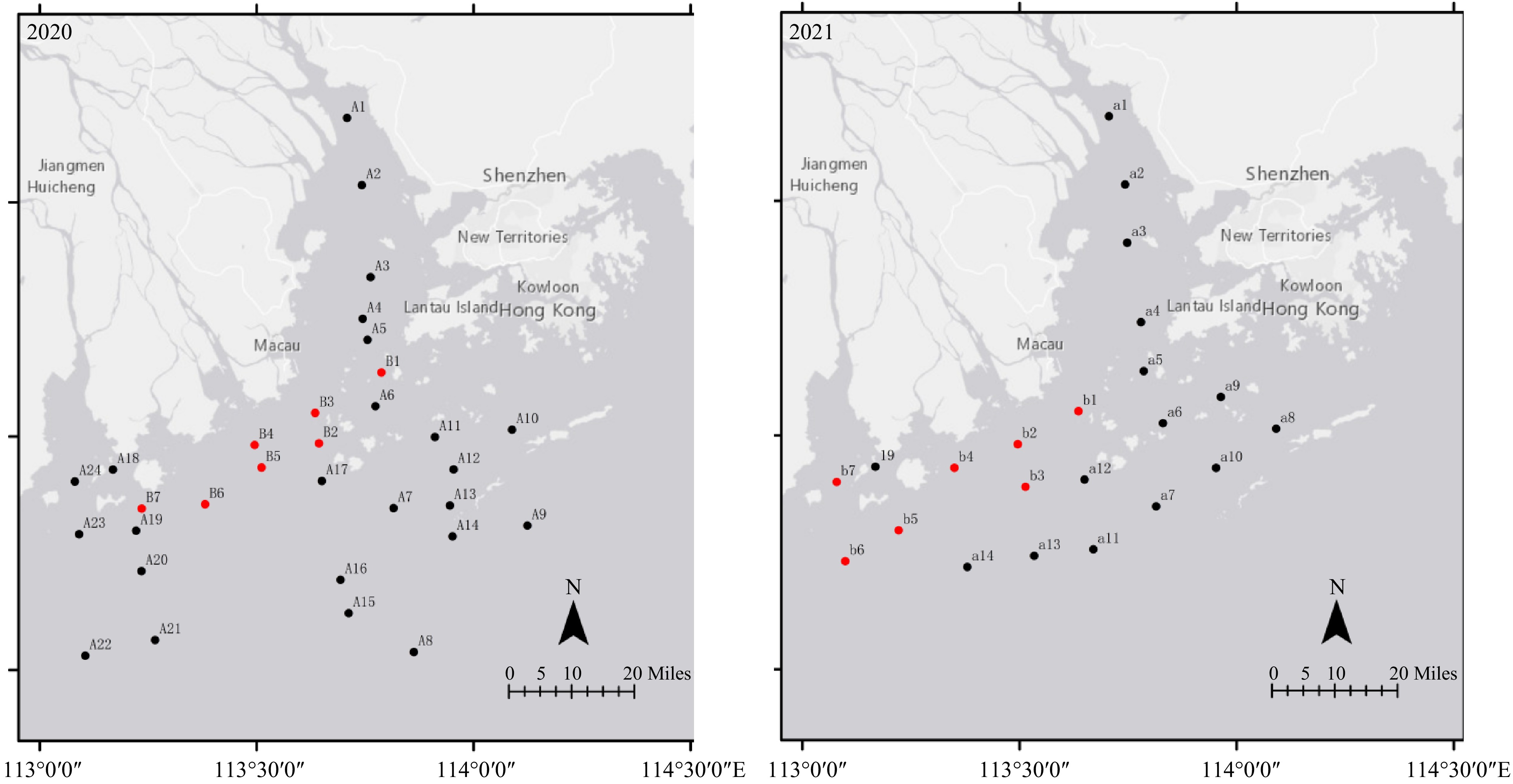
Figure 1. Distribution of macrobenthos sampling sites in the Pearl River Estuary (Note: red sites are hypoxic sites)
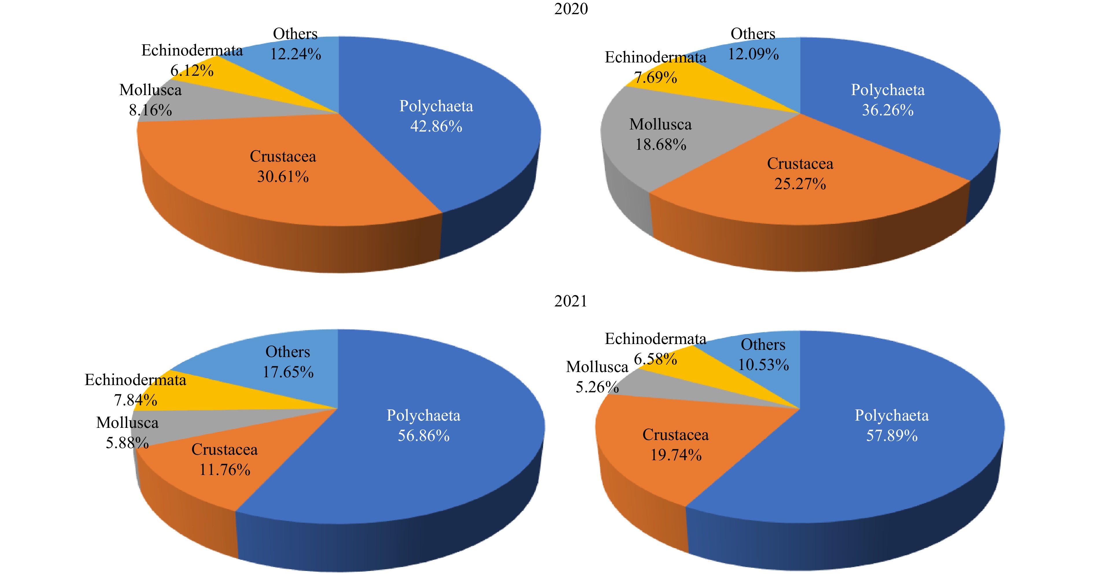
Figure 2. Species composition of macrobenthos in 2020 and 2021 (left: hypoxic area; right: non-hypoxic area)

Figure 3. Mean abundance and biomass of different macrobenthos faunas in hypoxic region and non-hypoxic region in 2020 and 2021
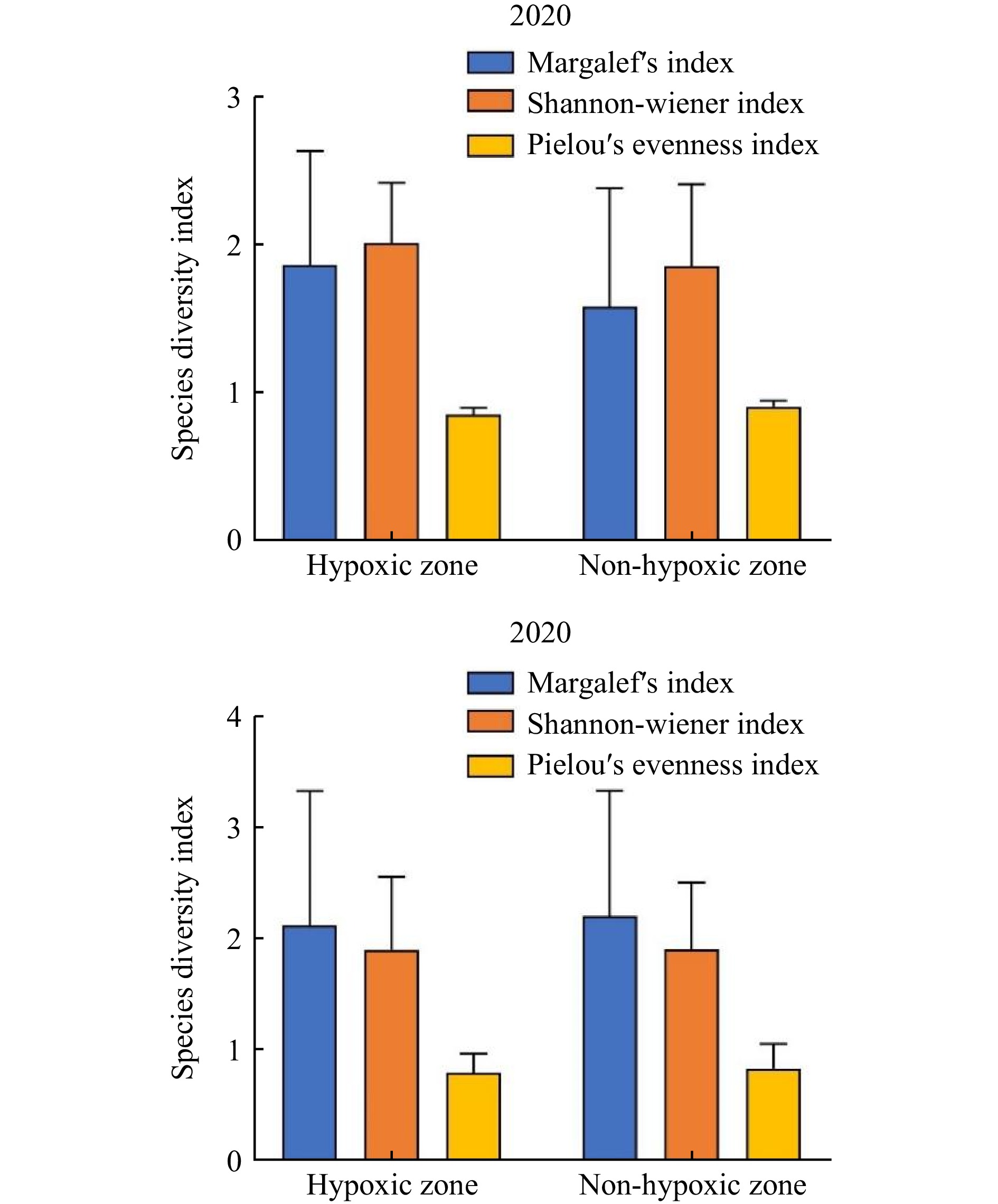
Figure 4. Mean species diversity index of macrobenthos in hypoxic and non-hypoxic area in 2020 and 2021
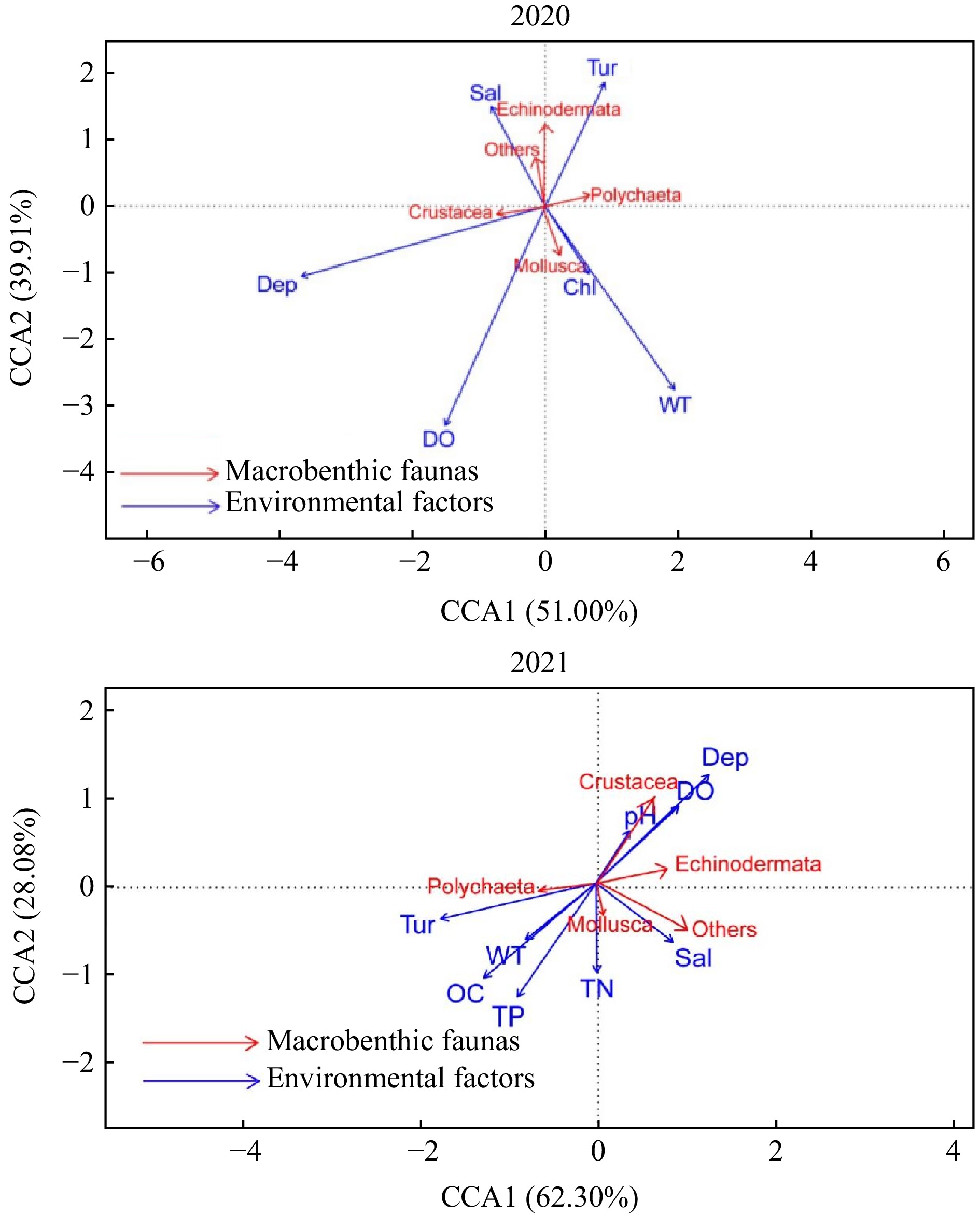
Figure 5. Canonical correspondence analysis of different macrobenthos faunas and environmental factors in 2020 and 2021
Table 1. Dominant macrobenthos species in hypoxic area and non-hypoxic area
Date region Species Dominance (Y) July in 2020 Hypoxic area Cossurella dimorpha 0.096 Sternaspis sculata 0.058 Neotrypaea japonica 0.052 Amphioplus sinicus 0.021 Non-hypoxic area Neotrypaea japonica 0.027 July in 2021 Hypoxic area Paraprionospio pinnata 0.190 Lintriolobus brevirostris 0.057 Neotrypaea japonica 0.027 Apionsoma trichocephala 0.026 Nephthys oligobranchia 0.021 Linopherus ambigua 0.021 Non-hypoxic area Neotrypaea japonica 0.094 Lintriolobus brevirostris 0.041 Paraprionospio pinnata 0.041  下载: 导出CSV
Table 2. Spearman correlation analysis between environmental factors
Dep WT DO Tur Chl Sal pH TN TP TOC Dep 1.000 WT −0.702** 1.000 DO 0.431** −0.138 1.000 Tur −0.742** 0.429** −0.482** 1.000 Chl −0.473** 0.432** 0.031 0.273 1.000 Sal 0.763** −0.840** 0.132 −0.512** −0.378* 1.000 pH 0.239 −0.134 0.658** −0.121 −0.464 0.364 1.000 TN −0.164 0.151 −0.456* 0.218 −0.393 −0.083 −0.106 1.000 TP −0.522* 0.388 −0.797** 0.429 0.179 −0.256 −0.419 0.768** 1.000 TOC −0.526* 0.505* −0.474* 0.571** −0.214 −0.535* −0.183 0.723** 0.708** 1.000 Note: ** correlation is significant with p<0.01; *correlation is significant with p<0.05.
下载: 导出CSV
Table 3. Spearman correlation analysis between environmental factors and macrobenthos
Dep WT DO Tur Chl Sal pH TN TP TOC Number of species −0.226 0.028 −0.213 0.106 −0.059 0.005 0.270 −0.121 −0.006 0.409 Total abundance −0.174 −0.029 −0.386** 0.112 −0.169 0.098 0.103 −0.248 −0.059 0.023 Total biomass −0.073 −0.232 −0.292* 0.031 −0.091 0.112 0.170 −0.084 −0.025 −0.111 Margalef’s index 0.053 −0.082 −0.001 −0.077 0.007 0.237 0.403 −0.419 −0.400 −0.158 Shannon-Wiener index 0.115 −0.253 −0.025 −0.106 0.050 0.290 0.048 −0.285 −0.247 −0.363 Pielou's evenness index 0.254 −0.082 0.349* −0.134 0.043 −0.124 −0.096 −0.029 −0.116 −0.033 Abundance of Polychaeta −0.267 0.236 −0.364* 0.175 0.266 −0.129 −0.150 −0.097 0.200 0.276 Biomass of Polychaeta −0.171 0.062 −0.470** 0.109 0.036 0.017 0.034 −0.241 0.053 0.201 Abundance of Mollusca 0.341 −0.046 0.258 −0.251 0.232 0.116 −0.338 −0.135 −0.439 −0.507 Biomass of Mollusca 0.239 −0.062 0.110 0.036 −0.158 −0.131 0.314 −0.829* −0.371 0.086 Abundance of Crustacea 0.256 −0.249 0.125 −0.084 −0.088 0.292 0.624** −0.334 −0.388 0.169 Biomass of Crustacea −0.161 −0.096 −0.108 −0.148 0.030 0.087 0.176 −0.262 −0.235 0.150 Abundance of Echinodermata −0.279 −0.112 −0.213 0.135 −0.090 0.227 0.342 −0.439 −0.586 −0.024 Biomass of Echinodermata −0.122 −0.018 0.033 −0.105 0.316 0.099 0.405 −0.095 −0.357 −0.238 Abundance of Others 0.022 −0.079 −0.229 0.060 0.065 0.151 0.160 0.076 0.091 −0.131 Biomass of Others 0.012 −0.223 −0.141 0.054 −0.221 0.245 0.300 0.214 0.250 −0.032 Note: ** the correlation is significant with p< 0.01; * the correlation is significant with p<0.05.
下载: 导出CSV
-
Benke A C, Huryn A D. 2010. Benthic invertebrate production—facilitating answers to ecological riddles in freshwater ecosystems. Journal of the North American Benthological Society, 29(1): 264–285, doi: 10.1899/08-075.1 Berger W H, Parker F L. 1970. Diversity of planktonic foraminifera in deep-sea sediments. Science, 168(3937): 1345–1347, doi: 10.1126/science.168.3937.1345 Bray J R, Curtis J T. 1957. An ordination of the upland forest communities of southern Wisconsin. Ecological Monographs, 27(4): 325–349, doi: 10.2307/1942268 Castellano G C, da Cunha Lana P, Freire C A. 2020. Euryhalinity of subtropical marine and estuarine polychaetes evaluated through carbonic anhydrase activity and cell volume regulation. Journal of Experimental Zoology. Part A. Ecological and Integrative Physiology, 333(5): 316–324, doi: 10.1002/jez.2357 Castrillón-Cifuentes A L, Zapata F A, Giraldo A, et al. 2023. Spatiotemporal variability of oxygen concentration in coral reefs of Gorgona Island (Eastern Tropical Pacific) and its effect on the coral Pocillopora capitata. PeerJ, 11: e14586, doi: 10.7717/peerj.14586 Chu J W F, Tunnicliffe V. 2015. Oxygen limitations on marine animal distributions and the collapse of epibenthic community structure during shoaling hypoxia. Global Change Biology, 21(8): 2989–3004, doi: 10.1111/gcb.12898 Clarke K R, Warwick R M. 2001. Changes in marine communities: an approach to statistical analysis and interpretation. Mount Sinai Journal of Medicine New York, 40(5): 689–692, doi: 10.2337/diacare.26.7.2005 (查阅网上资料,未找到本条文献信息,请确认) Coffin M R S, Courtenay S C, Pater C C, et al. 2018. An empirical model using dissolved oxygen as an indicator for eutrophication at a regional scale. Marine Pollution Bulletin, 133: 261–270, doi: 10.1016/j.marpolbul.2018.05.041 Cognetti G, Maltagliati F. 2000. Biodiversity and adaptive mechanisms in brackish water fauna. Marine Pollution Bulletin, 40(1): 7–14, doi: 10.1016/S0025-326X(99)00173-3 Dauer D M. 1993. Biological criteria, environmental health and estuarine macrobenthic community structure. Marine Pollution Bulletin, 26(5): 249–257, doi: 10.1016/0025-326X(93)90063-P Dzwonkowski B, Fournier S, Reager J T, et al. 2018. Tracking sea surface salinity and dissolved oxygen on a river-influenced, seasonally stratified shelf, Mississippi Bight, northern Gulf of Mexico. Continental Shelf Research, 169: 25–33, doi: 10.1016/J.CSR.2018.09.009 Eby L A, Crowder L B. 2002. Hypoxia-based habitat compression in the Neuse River Estuary: context-dependent shifts in behavioral avoidance thresholds. Canadian Journal of Fisheries and Aquatic Sciences, 59(6): 952–965, doi: 10.1139/F02-067 Fajardo M, Andrade D, Bonicelli J, et al. 2018. Macrobenthic communities in a shallow normoxia to hypoxia gradient in the Humboldt upwelling ecosystem. PLoS One, 13(7): e0200349, doi: 10.1371/journal.pone.0200349 Friedrich J, Janssen F, Aleynik D, et al. 2014. Investigating hypoxia in aquatic environments: diverse approaches to addressing a complex phenomenon. Biogeosciences, 11(4): 1215–1259, doi: 10.5194/BG-11-1215-2014 Galic N, Hawkins T, Forbes V E. 2019. Adverse impacts of hypoxia on aquatic invertebrates: a meta-analysis. Science of the Total Environment, 652: 736–743, doi: 10.1016/j.scitotenv.2018.10.225 He Biyan, Dai Minhan, Zhai Weidong, et al. 2014. Hypoxia in the upper reaches of the Pearl River Estuary and its maintenance mechanisms: a synthesis based on multiple year observations during 2000–2008. Marine Chemistry, 167: 13–24, doi: 10.1016/J.MARCHEM.2014.07.003 Hourdez S, Weber R F, Green B N, et al. 2002. Respiratory adaptations in a deep-sea orbiniid polychaete from Gulf of Mexico brine pool NR-1: metabolic rates and hemoglobin structure/function relationships. Journal of Experimental Biology, 205(11): 1669–1681., doi: 10.1242/jeb.205.11.1669 Karatayev A Y, Burlakova L E, Mehler K, et al. 2018. Biomonitoring using invasive species in a large lake: Dreissena distribution maps hypoxic zones. Journal of Great Lakes Research, 44(4): 639–649, doi: 10.1016/j.jglr.2017.08.001 Kennish M J. 1997. Pollution Impacts on Marine Biotic Communities. Boca Raton: CRC Press. Lamont P A, Gage J D. 2000. Morphological responses of macrobenthic polychaetes to low oxygen on the Oman continental slope, NW Arabian Sea. Deep-Sea Research Part II: Topical Studies in Oceanography, 47(1-2): 9–24, doi: 10.1016/S0967-0645(99)00102-2 Li Gang, Liu Jiaxing, Diao Zenghui, et al. 2018. Subsurface low dissolved oxygen occurred at fresh- and saline-water intersection of the Pearl River estuary during the summer period. Marine Pollution Bulletin, 126: 585–591, doi: 10.1016/j.marpolbul.2017.09.061 Li Xiuqin, Lu Chuqian, Zhang Yafeng, et al. 2020. Low dissolved oxygen in the Pearl River estuary in summer: long-term spatio-temporal patterns, trends, and regulating factors. Marine Pollution Bulletin, 151: 110814, doi: 10.1016/j.marpolbul.2019.110814 Liao Y B, Shou L, Jiang Z B, et al. 2019. Effects of fish cage culture and suspended oyster culture on macrobenthic communities in Xiangshan Bay, a semi-enclosed subtropical bay in eastern China. Marine Pollution Bulletin, 142: 475–483, doi: 10.1016/J.MARPOLBUL.2019.03.065 Lu Lin. 2005. The relationship between soft-bottom macrobenthic communities and environmental variables in Singaporean waters. Marine Pollution Bulletin, 51(8-12): 1034–1040, doi: 10.1016/j.marpolbul.2005.02.013 Luo Chen, Routh J, Luo Dinggui, et al. 2021. Arsenic in the Pearl River Delta and its related waterbody, South China: occurrence and sources, a review. Geoscience Letters, 8(1): 12., doi: 10.1186/s40562-021-00185-9 Margalef R. 1958. Information theory in biology. General System, 3: 36–71 Maury O, Poggiale J C. 2013. From individuals to populations to communities: a dynamic energy budget model of marine ecosystem size-spectrum including life history diversity. Journal of Theoretical Biology, 324: 52–71, doi: 10.1016/j.jtbi.2013.01.018 Mutlu E, Çinar M E, Ergev M B. 2010. Distribution of soft-bottom polychaetes of the Levantine coast of Turkey, eastern Mediterranean Sea. Journal of Marine Systems, 79(1-2): 23–35, doi: 10.1016/j.jmarsys.2009.06.003 Ni Xiaobo, Zhou Feng, Zeng Dingyong, et al. 2023. Long-term observations of hypoxia off the Yangtze River Estuary: toward prediction and operational application. Frontiers in Ocean Observing, 36(S1): 40–41, doi: 10.5670/oceanog.2023.s1.13 Pandiya rajan R S, Jyothibabu R, Arunpandi N, et al. 2021. Macrobenthos community response to the seasonal hypoxia associated with coastal upwelling off Kochi, along the Southwest coast of India. Continental Shelf Research, 224: 104450, doi: 10.1016/j.csr.2021.104450 Pielou E C. 1975. Ecological Diversity. New York: Wiley, 1–165. Popchenko V I. 1971. Consumption of Oligochaeta by fishes and invertebrates. Journal of Icbtyology, 11(1): 75–80. (查阅网上资料, 未找到本条文献刊名全写, 请确认) Powilleit M, Kube J. 1999. Effects of severe oxygen depletion on macrobenthos in the Pomeranian Bay (southern Baltic Sea): a case study in a shallow, sublittoral habitat characterised by low species richness. Journal of Sea Research, 42(3): 221–234, doi: 10.1016/S1385-1101(99)00032-5 Rabalais N N, Baustian M M. 2020. Historical shifts in benthic infaunal diversity in the northern Gulf of Mexico since the appearance of seasonally severe hypoxia. Diversity, 12(2): 49, doi: 10.3390/d12020049 Rakocinski C F, Menke D P. 2016. Seasonal hypoxia regulates macrobenthic function and structure in the Mississippi Bight. Marine Pollution Bulletin, 105(1): 299–309, doi: 10.1016/j.marpolbul.2016.02.006 Ritter C, Montagna P A, Applebaum S. 2005. Short-term succession dynamics of macrobenthos in a salinity-stressed estuary. Journal of Experimental Marine Biology and Ecology, 323(1): 57–69, doi: 10.1016/j.jembe.2005.02.018 Ryu J, Khim J S, Kang S G, et al. 2011. The impact of heavy metal pollution gradients in sediments on benthic macrofauna at population and community levels. Environmental Pollution, 159(10): 2622–2629, doi: 10.1016/j.envpol.2011.05.034 Shannon C E, Weaver W. 1949. The Mathematical Theory of Communication. Urbana: University of Illinois Press, 1–144. Shivarudrappa S K, Rakocinski C F, Briggs K B. 2019. Vertical distribution of macrobenthos in hypoxia-affected sediments of the northern Gulf of Mexico: applying functional metrics. Estuaries and Coasts, 42(1): 250–263, doi: 10.1007/s12237-018-0446-z Taft O W, Haig S M. 2005. The value of agricultural wetlands as invertebrate resources for wintering shorebirds. Agriculture, Ecosystems & Environment, 110(3–4): 249–256, doi: 10.1016/j.agee.2005.04.012 Ueda K. 2013. Modeling of dissolved oxygen concentration recovery in water bodies and application to hypoxic water bodies. World Environment, 3(2): 52–59 Wei Hao, He Yunchang, Li Qingji, et al. 2007. Summer hypoxia adjacent to the Changjiang Estuary. Journal of Marine Systems, 67(3–4): 292–303, doi: 10.1016/j.jmarsys.2006.04.014 Zhou Weihua, Yuan Xiangcheng, Long Aimin, et al. 2014. Different hydrodynamic processes regulated on water quality (nutrients, dissolved oxygen, and phytoplankton biomass) in three contrasting waters of Hong Kong. Environmental Monitoring and Assessment, 186(3): 1705–1718, doi: 10.1007/s10661-013-3487-6 -


 DownLoad:


 点击查看大图
计量
- 文章访问数: 16
- HTML全文浏览量: 5
- 被引次数: 0

