

Spatial dynamics of phytoplankton assemblages and organic carbon stock in the highly productive Amundsen Sea Polynya and adjacent seasonal ice zone
-
Abstract: Polynyas and their adjacent seasonal ice zones (SIZs) represent the most productive regions in the Southern Ocean, supporting unique food webs that are highly sensitive to climate change. Understanding the dynamics of phytoplankton and the carbon pool in these areas is crucial for assessing the role of the southern ocean in global carbon cycling. During the late stage of an algal bloom, seawater samples were collected at 14 stations were collected in the Amundsen Sea Polynya (ASP) and adjacent SIZ. Using nutrients, phytoplankton pigments, organic carbon (OC), remote sensing data, and physicochemical measurements, as well as CHEMTAX model simulations, we investigated the response of the phytoplankton crops, taxonomic composition, and OC pool to environmental factors. Our analyses revealed that hydrodynamic regimes of the polynya, adjacent SIZs and open sea were regulated by the regionally varying intrusion of Circumpolar Deep Water, photosynthetically active radiation and sea ice melt water. The ASP exhibited the highest seasonal nutrient utilization rates (ΔN =
1059 ± 386 mmol/m2, ΔP = 50 ± 17 mmol/m2 and ΔSi = 956 ± 904 mmol/m2), while the open sea had lower rates. The integrated chlorophyll a (Chl a) concentrations at depths of 0–200 m ranged from 20.4 mg/m2 to1420.0 mg/m2 and peaked in the polynya. In the study area, Haptophytes P. antarctica was the dominant functional group (34% ± 27%), and diatoms acted as a secondary contributor (23% ± 14%). The major functional group and particulate OC (POC) contributor varied from diatoms (36% ± 12%) in the open sea to haptophytes (48% ± 31%) in the polynya waters. Strong light conditions and microelement limitations promoted the dominance of P. antarctica (low Fe forms) dominance in the ASP. The strong correlations between the POC and Chl a concentrations suggest that the POC was primarily derived from phytoplankton, while the dissolved OC (DOC) was influenced by consumer activity and water mass transport. In addition, the transport of OC in the upper 200 m of the water column within the ASP was quantified, revealing the predominantly westward fluxes for both DOC (9.0 mg OC·m−2·s−1) and POC (7.2 mg OC·m−2·s−1). The latitudinal transport exhibited the northward transport of DOC (8.1 mg OC·m−2·s−1) and southward transport of POC (4.3 mg OC·m−2·s−1) movement. These findings have significant implications for enhancing our understanding of how hydrodynamics influence OC cycling in polynya regions. -
1. Introduction
The Southern Ocean serves as a significant sink for atmospheric CO2 (Long et al., 2021). Despite encompassing only 30% of the global ocean surface, it accounts for approximately 40% of the oceanic uptake of anthropogenic CO2 (Takahashi et al., 2009; Gruber et al., 2019). This disproportionate role in carbon sequestration arises from its distinctive physical and biological features, including the formation of deep water, extensive sea ice dynamics, and elevated primary productivity in coastal and shelf regions (Arrigo et al., 2008). Particularly noteworthy are the polynyas, which stand out as biological hotspots, exhibiting intense phytoplankton blooms and active biogeochemical cycling (Arrigo and van Dijken, 2003; Lee et al., 2017). Understanding the carbon cycling in these polynyas is crucial for assessing the Southern Ocean's role in carbon sequestration and its response to ongoing climate variations.
The Amundsen Sea Polynya (ASP) is the most productive among 46 identified coastal polynyas (Arrigo et al., 2015). This is driven by seasonal sea ice melt, nutrient-rich winter water, and iron inputs from nearby melting ice sheets and benthic sediments (Van Manen et al., 2022). Massive algal blooms further lead to active high trophic level biological activities in the ASP (Arrigo and van Dijken, 2003; Hu et al., 2023; Kim et al., 2016, 2019; St-Laurent et al., 2017; Randall-Goodwin et al., 2015; Swalethorp et al., 2019; Yager et al., 2016; Yang et al., 2019). However, minimal carbon sequestration was observed in the ASP, and lower than 1.5% of the primary productivity-derived particulate organic carbon (POC) could be exported out of the ~400 m depth range and reach the bottom (Lee et al., 2017; Reigstad and Wassmann, 2007). Lee et al. (2017) speculated that most of the POC in the euphotic layer was converted into non-sinking forms, such as fine suspended particles or gelatinous colonies of bloom algae, dissolved inorganic carbon (DIC), or dissolved organic carbon (DOC)) (Lee et al., 2016, 2017; Reigstad and Wassmann, 2007). The absence of bottom water formation due to the intrusion of Circumpolar Deep Water (CDW) and strong lateral transport of non-sinking materials further limits the carbon sequestration capacity in the ASP, differing significantly from regions such as the Prydz Bay (Yu et al., 2024) and the Ross Sea polynyas (Sweeney et al., 2000). Thus, accurately assessing the variations in phytoplankton activity within this polynya and its adjacent waters, as well as the impact of the hydrodynamic conditions on the spatial distribution and transport of the organic carbon pool within the polynya, is particularly important for gaining a better understanding of the OC cycle therein.
Moreover, ecological and biogeochemical processes in the seasonal ice zone (SIZ) outside this polynya remain poorly understood. This knowledge gap is largely due to the limitations of satellite data and the technical challenges associated with sampling in ice-covered regions (Arrigo et al., 2008). Additionally, light limitation caused by sea ice has traditionally been thought to inhibit phytoplankton growth (Joy-Warren et al., 2019). However, recent studies have revealed the occurrence of substantial algal growth even under dense pack ice or within sea ice itself (Arrigo et al., 2012; Smith et al., 2014; Yu et al., 2024). Notably, the POC fluxes in the ASP and neighboring SIZ during the austral summer have been found to be comparable, which is driven by the more efficient export of the siliceous biological carbon pump in the SIZ (Kim et al., 2016). These finding highlight the critical need for detailed investigations in ice-covered regions to better understand the ecological and biogeochemical dynamics in such regions.
Significant surface warming and rapid sea ice retreat are occurring in the Amundsen Sea (Schoof, 2010), as well as CDW intrusion-induced glacier melting and thinning in the ASP (glacier mass loss of around 181.2 Gt a−1; Pritchard et al., 2012), further affecting the sea ice dynamics, light availability, water stratification and nutrient supply in the euphotic layer (Arrigo et al., 2012; Ha et al., 2014; Jenkins et al., 2016; Nakayama et al., 2013). Moreover, annual variations in phytoplankton crops and community structures have also been observed (Ge et al., 2024; Hyun et al., 2016; Kim et al., 2016; Lee et al., 2017). The high rates of carbon transformation within the polynya environment are largely driven by the circulation and migration of water masses, solar radiation, and ice-sea interactions (Hu et al., 2023; Lee et al., 2017; Yager et al., 2016). Thus, long-term, continuous, and high resolution studies on the responses of phytoplankton communities and carbon cycling to environment changes in the polynya-seasonal ice zone-open sea continuum are essential.
In this study, we aimed to elucidate the spatial distribution patterns of phytoplankton taxonomic compositions and organic carbon stock variations along the open sea-SIZ-polynya continuum. By integrating in situ hydrological observations, satellite remote sensing data, and analyses of phytoplankton pigments and organic carbon concentrations, we conducted a comprehensive assessment of the biogeochemical dynamics in the study area. Our research expands upon previous studies of phytoplankton primary production and phytoplankton-derived OC variations by exploring the fine-scale relationships between physical forces and biological responses (e.g., Ge et al., 2024; Kim et al., 2016; Lee et al., 2016, 2017; Park et al., 2019; Yager et al., 2016). The findings of this study will enhance our understanding of how changing environmental conditions (e.g., hydrodynamic conditions and sea ice dynamics) affect phytoplankton activity and the OC pool in polar regions, informing global climate models and predictions of the future oceanic carbon sequestration capacity.
2. Material and methods
2.1 Field sampling and oceanographic measurements
During the late stage of an algal bloom (NASA’s Ocean Color website,
https://oceancolor.gsfc.nasa.gov/l3/ ), water samples were collected at 14 stations in the ASP-SIZ-open sea continuum during the 36th Chinese National Antarctica Research Expedition (CHINARE) aboard the R/V Xuelong (Fig. 1a). The survey was conducted in the mid-summer period from Jan. to Feb. 2020, spanning latitudes of 66°S to 74°S and longitudes of 112°W to 120°W. Within the ASP, two research transects were established along the north-south direction (A11-04, A11-02, and A11-00) and the east-west direction (A9-01, A11-02, and A4-03), as well as two additional sites in the western ASP. Spatially, these stations encompassed nearly the entire ice-free area of the ASP during the sampling period. Based on the sea ice conditions at the time of the field investigation and considering the convenience of sampling, three stations (A3-07, A3-06, and A3-05) were established in the SIZ in front of the Dotson Trough (DT), where the sea ice concentration was relatively low (Fig. 1b). In the open sea, where the water properties were relatively uniform, four stations (A3-10, A3-08, A4-09, and A4-07) were established (Fig. 1b). To characterize the full water column, measurements of the temperature, salinity, and density were obtained using a pre-calibrated Sea-Bird SBE-9/11 plus Conductivity-temperature-depth system (CTD, Bellevue, U.S.A.). Full depth current profiles, including the flow velocity and direction, were gathered using a lowered acoustic Doppler current profiler (LADCP, TRDI WH300, C.A., U.S.A.) with a downward-looking transducer mounted on the CTD package. The near-surface currents were measured using a ship-mounted 38 kHz Ocean Surveyor and a 300 kHz Workhorse Mariner (TRDI, C.A., U.S.A.). Water samples were collected at the surface, 25 m, 50 m, 100 m, 200 m, and the chlorophyll maximum depth using a Rosette multi-sampler (General Oceanics, F.L., U.S.A.). The nutrients, phytoplankton pigments, dissolved organic carbon (DOC) and particulate organic carbon (POC) of the samples were subsequently analyzed. Figure 1. Sampling locations and hydrographic conditions in the Amundsen Sea. a. Study area bathymetry and sampling stations occupied during the 36th Chinese National Antarctic Research Expedition (CHINARE) from January to February 2020. Transect L (Leg L) extends southeastward from the open ocean, traversing the sea ice zone (SIZ) and polynya, to the DIS front. The Dotson Trough (DT) is delineated by a black line at the shelf break. b. Sea ice concentration during the sampling period. c. Vertical profiles of potential temperature (℃) along Transect L (0–250 m). d. Vertical profiles of salinity (‰) along Transect L (0–250 m). e. Vertical profiles of potential temperature (℃) along Transect L (whole water column). f. Vertical profiles of salinity (‰) along Transect L (whole water column). Water masses: AASW: Antarctic Surface Water; WW: Winter Water; mCDW: Modified Circumpolar Deep Water; CDW: Circumpolar Deep Water; ACC: Antarctic Circumpolar Current; RG: Ross Gyre; CC: Coastal current; GIS: Getz Ice Shelf; DIS: Dotson Ice Shelf; CIS: Crosson Ice Shelf; TIS: Thwaites Ice Shelf. The water circulations in Plot a are according to Kim et al. (2017) and Nakayama et al. (2018), red arrows represent water currents, and yellow arrows represent the intrusion of CDW onto the Amundsen Sea shelf.
2.2 Nutrient analysis and utilization rates
The dissoved samples analyzed for inorganic nutrients, including nitrate, nitrite, phosphate, and silicate, were filtered using pre-washed cellulose acetate membrane filters (0.45 µm). The filtered samples were stored in a freezer until analysis in the onshore laboratory. The nutrient concentrations were measured using a continuous flow analyzer (Skalar Analytical, Breda, The Netherlands) following the method of Grasshoff et al. (1999). The detection limits were 0.1 μM for nitrate, nitrite, and silicate, and 0.03 μM for phosphate, respectively (Feng et al., 2022b).
The nutrient utilization ratios were calculated according to the method of Rubin et al. (1998), using seasonal depletions of the dissolved inorganic nutrients, including the total nitrogen (TN) (i.e., NO3-N and NO2-N), PO4-P, and SiO3-Si in the surface mixed layer. These estimates were based on depth-integrated depletions of nutrients in summer from the surface layers down to the Tmin layer at each station. The Tmin layer represents the remnant winter water, and it had the lowest observed temperature in the water column. This methodology assumes that the nutrient depletion in the summer is primarily driven by biological processes initiated since the previous winter and that the upper water column remains well stratified. In this study, the temperature profiles of the study area revealed the presence of a distinct remnant winter water (WW) layer between the Antarctic Surface Water (AASW) and the CDW (Figs 1c–f). This layer, which is approximately 100 m thick, was characterized by significantly low temperatures, with minimum values (Tmin) ranging from –1.27℃ to –1.78℃ observed at depths between 75 m and 200 m (Figs 1c–f). The stratification of the upper water column was further enhanced by the intrusion and uplift of the warm modified Circumpolar Deep Water (mCDW ) and contributions from glacial and/or sea ice melt water in both the mesopelagic zone of the open sea area and the continental shelf region (Fig. 1). The utilizations of the nutrients were calculated using equation as follows:
$$ {\mathrm{Nutrient}}_{\mathrm{utilization}} = {\int^{z*}_0 }\Delta\left[\mathrm{C}\right]\mathrm{d}z = \int^{z*}_0 ({\left[\mathrm{C}\right]}_{\mathrm{win}}-{\left[\mathrm{C}\right]}_{\mathrm{sum}})\mathrm{d}z {\mathrm{,}} $$ (1) where Nutrientutilization is the net seasonal utilization of nutrients,
$ \Delta\left[\mathrm{C}\right] $ is the seasonal variations in the nutrient concentrations from the surface to the Tmin layer (z*), and the subscripts win and sum denote winter and summer.2.3 Phytoplankton pigment analysis
The samples used for the phytoplankton pigment were filtered through GF/F filters (0.7 μm, Whatman, New Castle, U.S.A.) under dim light and low vacuum pressure (<0.5 atm, 1 atm = 101 325 Pa), and were stored at −80℃ until analysis in the onshore laboratory. In the laboratory, the matter on the filters was extracted using 3 ml of acetone and was ultrasonicated in an ice bath for 30 seconds following the method of Feng et al. (2022b). The mixtures were then stored at −20℃ for 2 h. To remove the debris, the extracts were filtered through 0.22 µm polytetrafluoroethylene (PTFE) syringe filters. The supernatants were evaporated to dryness under a gentle stream of N2 and were re-dissolved in 300 μL of a methanol and water mixture (9:1 v/v). The extraction process was completed within 4 h to minimize pigment degradation.
The phytoplankton pigments were analyzed using an ultra performance liquid chromatography (UPLC) system (Acquity H-Class, Waters Corp., Milford, USA) equipped with a C18 column (50 × 2.1 mm i.d., 1.7 μm, Acquity UPLC® BEH), a photo-diode array (PDA) eλ detector, and a fluorescence (FLR) detector (excitation at 440 nm, emission at 660 nm). A modified binary gradient elution program, based on Zapata et al. (2000) and adapted by Feng et al. (2022a, 2022b), was utilized. The pigments were identified and quantified by comparing their retention times, absorption spectra, and peak areas with those of authentic standards (DHI Water and Environment, Hørsholm, Denmark). The analyzed pigments included chlorophyll a (Chl a), chlorophyll b (Chl b), chlorophyll c3 (Chl c3), chlorophyll c2 (Chl c2), pheophytin a (Phytin-a), pheophorbide a (Phide-a), alloxanthin (Allo), 19’-butanoyloxyfucoxanthin (But-fuco), fucoxanthin (Fuco), 19′-hexanoyloxyfucoxanthin (Hex-fuco), peridinin (Peri), violaxanthin (Vio), lutein, and zeaxanthin (Zea). The detection limit of the method was 3.1 ng, with a precision of better than 5% at a standard concentration of
0.0219 μg/L (e.g., Chl a).2.4 Pigment-based phytoplankton taxonomic composition
Utilizing the CHEMTAX program (Version 1.95) as outlined by Wright et al. (2009) and Feng et al. (2022a, 2022b), in this study, we employed eight diagnostic pigments to characterize the phytoplankton community and estimate the relative proportions of the different algal types in relation to the total Chl a concentration (Table 1). The following specific pigments serve as indicators for distinct algal groups: Chl c3 and Chl b are indicative of haptophytes (mainly P. antarctica) and green flagellates, respectively, whereas Chl c2 and Fuco are shared between diatoms and P. antarctica. Allo, Peri, and Zea are characteristic of cryptophytes, dinoflagellates, and cyanobacteria.
Table 1. Ratios of concentrations of diagnostic pigments to chlorophyll a (Chl a) used for CHEMTAX analysisMatrix Chl c3 Peri Fuco Vio Hex-fuco Allo Lutein Chl b Chl a
Initial matrixChlorophytes 0.00 0.00 0.00 0.03 0.00 0.00 0.22 0.18 1.00 Cryptophytes 0.00 0.00 0.00 0.00 0.00 0.22 0.00 0.00 1.00 Diatoms-A 0.00 0.00 0.57 0.00 0.00 0.00 0.00 0.00 1.00 Diatoms-B 0.03 0.00 1.02 0.00 0.00 0.00 0.00 0.00 1.00 Dinoflagellates 0.00 0.54 0.00 0.00 0.00 0.00 0.00 0.00 1.00 Haptophytes (high Fe) 0.13 0.00 0.08 0.00 0.40 0.00 0.00 0.00 1.00 Haptophytes (low Fe) 0.27 0.00 0.02 0.00 1.10 0.00 0.00 0.00 1.00
Final matrixChlorophytes 0.00 0.00 0.00 0.06 0.00 0.00 0.15 0.17 1.00 Cryptophytes 0.00 0.00 0.00 0.00 0.00 0.28 0.00 0.00 1.00 Diatoms-A 0.00 0.00 0.75 0.00 0.00 0.00 0.00 0.00 1.00 Diatoms-B 0.04 0.00 1.08 0.00 0.00 0.00 0.00 0.00 1.00 Dinoflagellates 0.00 0.64 0.00 0.00 0.00 0.00 0.00 0.00 1.00 Haptophytes (high Fe) 0.10 0.00 0.10 0.00 0.43 0.00 0.00 0.00 1.00 Haptophytes (low Fe) 0.21 0.00 0.02 0.00 1.36 0.00 0.00 0.00 1.00 Notes: Initial ratios before analysis (a) and optimized ratios after analysis (b). Chl c3: chlorophyll c3; Peri: peridinin; Hex-fuco: 19’-hexanoyloxyfucoxanthin; Fuco:fucoxanthin; Vio: violaxanthin; Allo: alloxanthin; Chl b: chlorophyll b, and Chl a: chlorophyll a | Show Table DownLoad:
CSV
DownLoad:
CSV
The CHEMTAX model functions by comparing the pigment compositions of the samples to a reference initial matrix of known pigment profiles for various phytoplankton taxa. Discrepancies between the initial matrix and actual field values often arise due to factors such as the light and nutrient conditions, which affect the pigment composition. To refine the pigment-algae matrix specific to the study area, the CHEMTAX program was iterated 60 times, generating a final matrix that was deemed to be representative of the true pigment composition. The initial and final matrix pigment ratios for seven target phytoplankton functional groups are presented in Table 1. In this analysis, the diatoms were categorized into two groups: Diatoms-A, comprised of Fragilariopsis spp., Chaetoceros spp., and Proboscia spp., and Diatoms-B, specifically representing Pseudo-nitzschia spp. Through further differentiation, the haptophytes (mainly P. antarctica) were mdivided into two forms, namely a high iron (Fe) form and a low Fe form, based on the relative proportions of Chl c3, Peri, and Hex-Fuco to the Chl a concentration, as well as their responses to the dissolved Fe levels. The methodology has been described in detail by Wright et al. (2010) and Alderkamp et al. (2012). The Chlorophytes evaluated in this CHEMTAX analysis are referred to as green flagellates bearing Chl b and are not assigned a distinct algal group (Peeken, 1997; Mendes et al., 2013).
2.5 Phytoplankton community size structure
Following the methodology established by Uitz et al. (2006, 2009), which leverages a comprehensive global pigment database to associate pigments with phytoplankton of varying sizes, we estimated the proportions of micro-, nano-, and picophytoplankton within an algal community using diagnostic pigment compositions and corresponding coefficients. Specifically, Peri and Fuco serve as diagnostic pigments for dinoflagellates and diatoms, respectively, which are categorized as microphytoplankton. Hex-fuco and But-fuco are indicative of chromophytes and nanoflagellates, representing nanoplankton; while Allo is a biomarker for cryptophytes, also classified as nanoplankton (Uitz et al., 2006). Additionally, Chl b and Zea are predominantly found in picoplankton, including green flagellates and cyanobacteria (Vidussi et al., 2001). The contributions of these size classes (i.e., micro-, nano-, and picophytoplankton) to the total Chl a stock were calculated using empirical formulas as follows:
$$ \mathrm{F}_{\mathrm{micro}} =(1.41[{\mathrm{Fuco}}]+1.41[{\mathrm{Peri}}])/[\Sigma {\mathrm{DP}}_{\mathrm{w}}] \mathrm{,} $$ (2) $$ \mathrm{F}_{\mathrm{nano}} =(1.27[{\mathrm{Hex}}{\text{-}}{\mathrm{fuco}}]+0.60[{\mathrm{Allo}}]+0.35[{\mathrm{But}}{\text{-}}{\mathrm{fuco}}])/[\Sigma {\mathrm{DP}}_{ \mathrm{w}} ]\mathrm{,} $$ (3) $$ \mathrm{F}_{\mathrm{pico}} =(0.86[{\mathrm{Zea}}]+1.01[{\mathrm{Chl}} b] )/[\Sigma \mathrm{DP}_{ \mathrm{w}} ]\mathrm{,} $$ (4) where [Fuco], [Peri], [Hex-fuco], [Allo], [But-fuco], [Zea], and [Chl b] are their own concentrations, and [ΣDPw] is the chl a concentration, which can be calculated as the weighted sum of the diagnostic pigment concentrations with the coefficients calculated from a global database of high-performance liquid chromatography (HPLC) pigment compositions (Uitz et al., 2006, 2009).
$$ \begin{split}[\Sigma \mathrm{DP}_{\mathrm{w}} ]=& 1.41[{\mathrm{Fuco}}]+ 1.41[{\mathrm{Peri}}]+ 1.27[{\mathrm{Hex}}{\text{-}}{\mathrm{fuco}}]+ 0.60[{\mathrm{Allo}}]+\\ &0.35[{\mathrm{But}}{\text{-}} {\mathrm{fuco}}]+0.86[{\mathrm{Zea}}[+1.01[{\mathrm{Chl}} b ]\mathrm{,}\\[-10pt]\end{split} $$ (5) These empirical formulas mitigate analytical uncertainties through normalization, offering a greater accuracy than individual accessory pigment concentrations for estimating phytoplankton size classes and facilitating comparisons with other data sources (Uitz et al., 2006, 2009). This approach has been effectively employed to identify and quantify the relative proportions of phytoplankton size classes in Antarctic waters (Uitz et al., 2006, 2009; Cheah et al., 2017; Wojtasiewicz et al., 2019).
2.6 POC and DOC analyses
The samples for POC analysis were filtered through a 0.7 μm pre-combusted GF/F filter (Whatman, New Castle, U.S.A.) under dim light conditions and were stored at −80℃ until analysis in the onshore laboratory. In the laboratory, the samples were exposed to acid fumes in a drying oven for 12 h to remove the inorganic carbon. Then, whey were rinsed with ultra-pure water and dried at 45℃. The analysis was performed using an elemental analyzer (vario MICRO cube, Elementar, Germany), with relative deviations of the organic carbon (OC) from replicate standard analyses of less than 0.1% (n = 6).
The samples for the DOC analysis were filtered through pre-combusted Whatman GF/F filters. The filtrate, combined with two drops of phosphoric acid, was stored in pre-combusted 20 mL glass ampoules at −20℃ until further analysis. The DOC measurements were conducted using a Shimadzu TOC-L analyzer with high temperature combustion. Milli-Q water samples were used as blanks to establish a baseline, and standard samples (42−45 µM C) from the Deep Sea Reference at the University of Miami were analyzed to ensure accuracy. Each sample was measured at least three times, and the analytical errors of the DOC were maintained within 5%.
2.7 Integrated water column values (nutrients, Chl a, POC, and DOC)
To mitigate statistical errors arising from unequal sampling depths when evaluating the regional distribution of nutrients, phytoplankton Chl a, POC, and DOC, we employed water column integral concentrations (Zhuang et al., 2014). These integrated values were calculated as follows:
$$ \mathrm{C}_{{\mathrm{int}}}= [\mathrm{C}_{1} (\mathrm{D}_{1}+ \mathrm{D}_{2})+ \mathrm{C}_{2} (\mathrm{D}_{3} -\mathrm{D}_{1} )+...+{\mathrm{C}}_{\mathrm{n}} (\mathrm{D}_{ \mathrm{n}}- \mathrm{D}_{ \mathrm{n}-1} )]/2\mathrm{,} $$ (6) where Dn is the measured depth of a layer, and Cn is the concentration of the target parameter (e.g., nutrients, Chl a, POC, and DOC concentrations) in that layer. The integrated values represent the stocks in the water column with a 200 m thickness per m2. This approach facilitates comprehensive assessment of the regional distributions of these parameters.
2.8 Remote sensing data and physical measurements of seawater properties
The photosynthetically active radiation (PAR) and euphotic layer depth (Zeu) data were obtained from remote sensing sources during the sampling period, which were averaged to eight days. The data were downloaded from SeaWiFs (
http://oceancolor.gsfc.nasa.gov/DOCS/seawifsparwfigs.pdf ) and Morel et al. (2007). The sea ice concentration data, sourced from remote sensing data, were acquired from the Polar View Bremen Sea Ice Database (http://seaice.uni-bremen.de/databrowser ). The data selected were within 30 km × 30 km of the observation stations to enable in-depth evaluation.To assess the contribution of fresh water to the euphotic layer in the study area, the percentage of sea ice meltwater (%MW) was calculated based on the salinity difference between the surface water (Ssurface) and deep water (Sdeep) at the same station (Mendes et al., 2018b; Costa et al., 2020). The equation used for this calculation is as follows:
$$ {\text{%}}{\mathrm{MW} }= \left(1 - \frac{{{{\text{S}}_{{\text{surface}}}} - 6}}{{{{\text{S}}_{{\text{deep}}}}-6}}\right) \times 100{\mathrm{,}} $$ (7) Sdeep (around 300 m depth) was assumed to be unaffected by sea ice dilution, and sea ice salinity was set to 6‰ (Ackley et al., 1979).
The mixed layer depth (MLD) was calculated by identifying the depth corresponding to the maximum buoyancy frequency of the water column, i.g., max (N2) (Carvalho et al., 2016), as follows:
$$ N^2 = - \frac{{\text{g}}}{\rho } \frac{{\partial \rho }}{{\partial {\text{z}}}} ({\mathrm{rad}}^2{\mathrm{s}}^{-2}), $$ (8) where g is gravity, and z is the water depth. The potential density of the seawater (ρ, kg m-3) was derived from the potential temperature, salinity, and pressure data. The stability of the water column (Estability) was further calculated as follows:
$$ {\mathrm{E}}_{\mathrm{stability}} = \frac{{{{\text{N}}^{\text{2}}}}}{{\text{g}}} (10^{-6}\; {\mathrm{rad}}^2\; {\mathrm{m}}^{-1}), $$ (9) The average values of Estability from 0 to 100 m depth were used to represent the horizontal variations in the water column stability at each station (Costa et al., 2020; Mendes et al., 2018b).
The arithmetical mean of the water velocity within each sampling layer was calculated using the LADCP data for the adjacent layers. For shallower depths (0 m, 25 m, 50 m, and 75 m), the mean velocity was calculated from 12.5 m above and 12.5 m below the target depth. For example, the mean velocity of the 25 m layer was averaged from 12.5 m to 37.5 m. For deeper depths (100 m, 150 m, and 200 m), the mean velocity was computed using data from 25 meters above and 25 m below the target depth.
2.9 Statistical analysis
The statistical analyses were performed using SPSS 24 (IBM, Armonk, NY, USA). The analyses included one-way analysis of variance (ANOVA). Pearson correlation analysis, two-tailed significance tests, and R-mode cluster analysis on a dataset comprised of physical and biochemical parameters (e.g., PAR, MLD, %MW, nutrient utilization rates, Chl a concentrations, and phytoplankton functional groups). These analyses aimed to elucidate theinternal relationships, such as the correlation coefficients (r), significance levels (p), and classification across different regions, with a significance threshold of p < 0.05. The depth-integrated nutrient utilization rates were calculated using Origin 2018 (OriginLab, Northampton, MA, USA).
3. Results
3.1 Regional environmental settings
In the ASP, adjacent SIZ, and open sea area, the hydrodynamic regimes are predominantly influenced by the Antarctic Circumpolar Current (ACC), coastal current, CDW, and Antarctic Surface Water (AASW) (Figs 1a, e and f). The CDW water in the open sea area is distinguished by its maximum temperature, reaching up to 1.8℃ (Zu et al., 2022). The intrusion of CDW onto the continental shelf and its interaction with the shelf waters result in slight reductions in temperature and salinity, and thus, it becomes mCDW (Figs 1e and f) Kim et al., 2017; Rignot et al., 2013). This southward-flowing mCDW is a major driver of the basal melting of the nearshore ice shelf (Pritchard et al., 2012). The physical properties of AASW, the temperature of which ranges broadly from approximately −1.5℃ to 2℃, are highly affected by solar radiation and the presence of sea ice. In the ASP, where the AASW is devoid of local sea ice, the AASW receives direct sunlight, leading to higher temperatures (around 1−2℃) and salinity values (Figs 1c and d). Conversely, in the SIZ, the AASW has lower temperatures and salinity values due to the influx of cold meltwater from sea ice and diminished solar exposure (Figs 1c and d). The remnant WW, located above the mCDW, is comprised of colder, saltier water formed by brine drainage and vertical convection during the previous winter (Figs 1c and d) (Kim et al., 2017). It is marked by a potential temperature of −1.5℃ and is located at depths of 50 m to 300 m (Figs 1c and e). The warmest water mass in the ASP region is the bottom mCDW (Fig. 1e). The density of the Amundsen Sea shelf water is less than that of the mCDW due to meltwater input from the ice shelves, promoting a stable hydrological environment on the shelf of ASP (Park et al., 2001; Meijers et al., 2010; Williams et al., 2010). Notably, significant sea ice was observed around stations A3-06, A3-05 and A3-07 during the sampling period (Fig. 1b).
The spatial distributions of the hydrological characteristics (MLD, PAR, Zeu, MW%, and Estability ) are shown in Fig. 2. Across the study area, the MLD varied from 12 m at station A3-03 in the ASP to 40 m at station A4-09 in the open sea area, with an average of 25 ± 8 m. As illustrated in Fig. 2b, the MLD was observed to be deeper in the northern open sea and southern polynya regions, while it was prevalently shallower MLD in the SIZ. The ice-free days generally exhibited a similar spatial pattern similar to the MLD (r = 0.65, p < 0.05). The MW% ranged from 0.7% to 6.8%, with an averaging of 3.9% ± 1.8%, and it was highest in the SIZ (Fig. 2c). The Estability ranged from 2.5 to 12.9, with an average of 6.7 ± 3.6, and it exhibited a distribution pattern similar to that of the MW% (r = 0.82, p < 0.01) (Fig. 2d), with the maximum and minimum values occurring at stations A3-05 (SIZ) and A11-00 (ASP), respectively. The ASP region had higher PAR values than the SIZ and open sea area (Fig. 2e). Furthermore, the Zeu exhibited significant positive correlations with both the Estability (r = 0.58, P < 0.05) and MW% (r = 0.53, P < 0.05).
 Figure 2. Hydrographic characteristics of the study area: a. Ice-free days (days elapsed between sea ice melting and sampling) b. mixed layer depth (MLD, m); (c. sea ice meltwater fraction (MW%, percentage); d. water column stability (Estability); e. photosynthetically active radiation (PAR); f. Euphotic zone depth (Zeu, m).
In the ASP, the speed and direction of the water current varied greatly. The stations located in the northeastern part of the ASP (i.e., Stations A11-04 and A4-03) were dominated by northward or northeastward flow with velocities of around 7 ± 3 cm/s, and thus, they acted as a major outflow window for the upper layers of the polynya water. Ha et al. (2014) reported that the water outflow flux on the western side of the DT accounts for around 33% of the inflow flux in the ASP. Conversely, southward and southeastward flows dominated at Stations A11-02 and A3-01 ((8 ± 1) cm/s), indicating inflows from the SIZ zone into the ASP. Coastal station A9-01 near the Getz Ice shelf exhibited the highest northwestward outflow, with a velocity of around (24 ± 5) cm/s; station A11-00 in front of the Dotson Ice shelf exhibited the weakest southwestward flow, with a velocity of around (6 ± 2) cm/s.
3.2 Stock and seasonal utilization of nutrients
Figure 3 presents the stock and seasonal utilization of the nutrients. In the study area, SiO3-Si was the most abundant nutrients and had the highest stock, ranging from 6.1 mol/m2 to 13.9 mol/m2 with an average concentration of (10.3 ± 2.1) mol/m2 in the top 200 m of the water column, and it generally increased toward south (Fig. 3c). In contrast, the inventories of the TN and PO4-P were significantly lower, with averages of (4.8 ± 0.9) mol/m2 and (0.3 ± 0.1) mol/m2, respectively. The TN and PO4-P were strongly correlated (r = 0.79, p < 0.01) and exhibited no significant differences among the ASP, SIZ, and open sea area. Ammonium contributed minimally to the total nitrogen nutrients, and was excluded when calculating the total nitrogen nutrient stocks and consumption.
 Figure 3. Spatial distributions of depth-integrated concentrations (a−c), seasonal utilization (d−f) and utilization ratios (g−i) of nutrients (TN: NO
$ _3^ - $ +NO$ _2^ - $ , silicates and phosphates)Regarding seasonal nutrient utilization, TNutilization varied from 0.37 mol/m2 to 1.40 mol/m2 (mean of 0.86 ± 0.38 mol/m2), Putilization ranged from 0.02 mol/m2 to 0.07 mol/m2 (mean of (0.04 ± 0.02) mol/m2), and Siutilization ranged from 0.11 mol/m2 to 2.23 mol/m2 (mean of (0.86 ± 0.62) mol/m2, Figs 3a–c). The seasonal nutrient utilization rates were higher in the ASP, and lower rates were observed in the open sea (Figs 3d–f). There were significant negative correlations between Siutilization and the ice-free days (r = −0.77, p < 0.01) and between Putilization and Estability (r = −0.55, p < 0.05).
The nutrient absorption ratios exhibited notable spatial variations. The ΔN/ΔP ranged from 8.9 to 32.2 (with an average of 22.4 ± 5.9), ΔN/ΔSi ranged from 0.2 to 10.9 (with an average of 2.1 ± 2.7), and ΔSi/ΔP ranged from 2.0 to 48.9 (with an average of 23.4 ± 13.9) (Figs 3g–i). The highest ΔN/ΔP and ΔN/ΔSi values both occurred in the ASP, while higher ΔSi/ΔP values were observed in the SIZ and open sea area (Figs 3g–i). Moreover, the length of the ice-free period was positively correlated with ΔN/ΔSi (r = 0.62, p < 0.05) and negatively correlated with ΔSi/ΔP (r = −0.61, p < 0.05).
3.3 Integrated concentrations of POC, DOC, Chl a, and their degradation products
Figure 4 illustrates the distributions of the integrated OC concentrations, phytoplankton Chl a, and its degradation products (DChl a, including pheophorbide a and pheophytin a) within the 0–200 m layer of the water column. In this study, it was found that the DOC was the predominant component of the total OC pool, ranging from 75.5 g/m2 to 146.8 g/m2, with an average of (106.8 ± 20.7) g/m2. The integrated POC concentrations varied from 8.6 g/m2 to 91.7 g/m2, with an average of (26.1 ± 24.3) g/m2. The average integrated DOC concentration was significantly higher in the SIZ compared to the ASP and open sea area (p < 0.05), whereas significantly higher integrated POC concentrations were observed in the ASP region compared to the other two regions (p < 0.05; Figs 4a and b). A significant negative correlation was observed between the integrated DOC and POC concentrations (r = −0.60, p < 0.05).
 Figure 4. Spatial variations in depth-integrated concentrations of DOC (g/m2) (a), POC (g/m2) (b), Chl a (c), Chl a degradation products (DChl a, mg/m2) (d), POC/Chl a ratio (e), and DChl a/Chl a ratio (f).
The integrated concentrations of phytoplankton Chl a and its degradation products exhibited variation trends similar to those of the integrated POC (r = 0.92, p < 0.01; Figs 4c and d). The Chl a concentrations ranged from 19.0 mg/m2 to
1408.5 mg/m2, with a mean of (223.9 ± 362.3) mg/m2. The concentrations of the Chl a degradation products were lower, ranging from 21.0 mg/m2 to 96.3 mg/m2, with a mean of (67.8 ± 26.4) mg/m2. Significantly higher concentrations of Chl a and its degradation products were recorded in the ASP region (p < 0.05), and there was no significant difference in the values in the SIZ and open sea area.3.4 Pigment-based phytoplankton taxonomic composition and community size structure
Figure 5 illustrates the phytoplankton taxonomic composition based on the CHEMTAX model calculation. Briefly, the dominant phytoplankton groups were Hapt-LowFe and Diatoms-B, accounting for 34% ± 26% and 23% ± 13% of the total, with variations ranging from 3% to 76% and from 3% to 51%, respectively. Comparatively, the proportions of the Chlorophytes (18% ± 13%), Dinoflagellates (13% ± 5%), Cryptophytes (12% ± 6%), Hapt-HighFe (1% ± 2%) and Diatoms-A (<1%) were substantially lower. Spatially, the Hapt-LowFe were more concentrated in the ASP region where the MW% was lower, and its proportion was significantly higher than that in the SIZ (p < 0.05). The Hapt-LowFe% exhibited positive correlations with the ice-free days (r = 0.60, p < 0.05), SiO3-Si stock (r = 0.54, p < 0.05), ΔN/ΔSi (r = 0.74, p < 0.01), and the concentrations of the integrated Chl a (r = 0.74, p < 0.01) and POC (r = 0.71, p < 0.01). However, they were negatively correlated with Zeu (r = −0.76, p < 0.01), Siutilization (r = −0.77, p < 0.01), and ΔSi/ΔP (r = −0.65, p < 0.05). Conversely, the Diatoms-B generally decreased toward the south, peaking at Site A3-10 in open sea area and dipping at Site A11-02 in the ASP. The proportion of Diatoms-B was significantly higher in open sea compared to the ASP (p < 0.05). The Diatoms-B% was positively correlated with ΔSi/ΔP (r = 0.68, p < 0.01) and negatively correlated with SiO3-Si stock (r = −0.73, p < 0.01) and ΔN/ΔSi (r = −0.66, p < 0.05). The other phytoplankton groups did not exhibit no clear spatial distributions, but the proportion of the Chlorophytes were slightly higher in the SIZ where the MW% was elevated (Figs 2c and 5c).
 Figure 5. Relative abundance of major phytoplankton taxonomic groups and community size structure in the study area. The contribution of Diatoms-A was negligible ( < 1%) and is not shown.
The phytoplankton community was dominated by a microsized (52% ± 20%) and nanosized (42% ± 20%) phytoplankton assemblage, and the picosized phytoplankton contributed only about 6% ± 2% (Figs 5g-i). The proportion of microphytoplankton, primarily composed of large cells such as diatoms, was positively correlated with the Diatoms-B (r = 0.76, p < 0.01), Estability (r = 0.54, p < 0.05), Zeu (r = 0.60, p < 0.01), Siutilization (r = 0.68, p < 0.01), and ΔSi/ΔP (r = 0.74, p < 0.01). However, there were negative correlation were observed between Fmicro% and the SiO3-Si stock (r = −0.62, p < 0.05) and the concentrations of the integrated Chl a (r = −0.61, p < 0.05) and POC (r = −0.63, p < 0.05). The proportion of microphytoplankton in the ASP was significantly lower than in the other two regions (p < 0.05; Fig. 5g). In contrast, the nanophytoplankton, mainly comprised of smaller algae such as Haptophytes, Dinoflagellates, and Cryptophytes, were significantly more abundant in the ASP than in the other two regions (p < 0.05; Fig. 5h). The proportion of nanophytoplankton was positively correlated with the SiO3-Si stock (r = 0.58, p < 0.05), ΔN/ΔSi (r = 0.71, p < 0.01), Hapto-LowFe% (r = 0.89, p < 0.01), and the concentrations of the integrated phytoplankton Chl a (r = 0.66, p < 0.05) and POC (r = 0.64, p < 0.05).
3.5 Results of PCA
PCA was employed to identify the key factors influencing the variations in the measured parameters (Fig. 6). The first two principal factors accounted for around 57% of the total variance in the dataset, with PC1 and PC2 contributing 41% and 16%, respectively. PC1 predominantly represents biological activity processes, encompassing phytoplankton crops and the taxonomic composition, the transformation of POC to DOC, and the utilization of various nutrients (Fig. 6a). In contrast, PC2 mainly reflects physical environmental features, such as changes in the water temperature, stratification, and MLD, which are driven by factors such as sunlight exposure and sea ice meltwater input (Fig. 6a). Overall, the PCA results indicate that the spatial zonation based on the sea ice density and ice-free days effectively explains the response of the phytoplankton activity across the ASP-SIZ-open sea continuum. The study area can be divided into three distinct regions based on the loading scores of each station (Fig. 6b).
 Figure 6. Principal component analysis (PCA) results. a. Variable loadings on Factor1 and Factor 2; b. sample scores on Factor 1 and Factor 2.
4. Discussion
The spatial distributions of the phytoplankton assemblages and OC pools across the ASP-SIZ-open sea continuum exhibited significant heterogeneity. The integrated POC and Chl a concentrations were markedly higher in the ASP than in the SIZ and open ocean (Figs 4b and c), indicating substantial differences in the phytoplankton crops among the different parts of the study area. The CHEMTAX analysis revealed that Hapt-LowFe was the dominant phytoplankton group, particularly within the ASP (Fig. 5a). The Hapt-LowFe also exhibited a strong positive correlation with the POC (r = 0.71, P < 0.01), highlighting its significant contribution to the ASP’s particulate carbon reservoir. These findings align with previous research documenting the substantial contribution of P. antarctica to the POC pools in the Amundsen and Ross Sea polynyas (Oliver et al., 2019; DiTullio et al., 2000) and the dominance of P. antarctica blooms in open ocean areas of the Cosmonaut Sea and Antarctic Peninsula (Feng et al., 2022b; Li et al., 2024). Collectively, these observations underscore the crucial role of small algal species in the carbon cycling and ecosystem functioning in the Southern Ocean.
4.1 Spatial heterogeneity of phytoplankton activity and environmental drivers
Phytoplankton crops and taxonomic community composition are strongly influenced by environmental factors, including the hydrodynamic conditions, nutrient availability (e.g., macronutrients and trace metals), and light regimes. Sea ice cover significantly impacts these ecosystems by altering the light penetration, water column stratification, and micronutrient supply (Boyd, 2002; Lannuzel et al., 2016; Mendes et al., 2018b; Li et al., 2024). Our PCA analysis revealed the occurrence of significant correlations between the Hapt-LowFe%, integrated Chl a and POC concentrations, and several key environmental variables: positive correlations with the ice-free days (r > 0.55, p < 0.05); and negative correlations with the water column stability (Estability, r < −0.73, p < 0.01), meltwater fraction (MW%, r < −0.55, p < 0.01), and nutrient utilization ratios (e.g., negative correlation with ΔSi/ΔP, r < −0.65, p < 0.05) (Fig. 6a). Furthermore, PCA distinguished three distinct regions based on these variables (Fig. 6b).
Druing the sampling period, the ASP was characterized by extended ice-free periods and low MW% values, and it probably experienced low iron conditions. Previous studies have suggested that the bio-essential dissolved iron supplied by the mCDW, benthic sediments, and ice shelf meltwater forms the critical foundation for sustaining the long-term phytoplankton blooms in the Amundsen Sea Polynya (Park et al., 2017; Sherrell et al., 2015; Van Manen et al., 2022). However, in this study, we did not observe a remarkable significant upwelling signal in the ASP's euphotic zone (Figs 1c and d). In addition, according to previous studies, most of the iron in the polynya exists in particulate form, and dissolved Fe can be rapidly scavenged by particles in the water and equilibrate with the labile particulate pool (Sherrell et al., 2015; Van Manen et al., 2022). In the polynya, high dissolved iron concentrations are typically observed below a depth of 100 m, such as in the bottom MCDW (>0.6 nM) and outflows (~0.5 nM) in the subsurface layer (Van Manen et al., 2022). Comparably, the dissolved iron concentration of the surface waters is approximately 0.19 nM in the polynya and around 0.17 nM in the open sea region (Ge et al., 2024; Sherrell et al., 2015; Van Manen et al., 2022). Additionally, satellite observations (NASA’s Ocean Color website, https://oceancolor.gsfc.nasa.gov/l3/) reveal that a phytoplankton bloom occurred and lasted for approximately two months (early December 2019 to February 2020). This prolonged bloom, coupled with substantial seasonal nutrient consumption (high TNutilization and Putilization; Figs 3d and e) and limited iron-rich meltwater, likely created a short-term low-iron environment. Nanophytoplankton (<20 μm), such as P. antarctica, cyanobacteria, green flagellates, and cryptophytes, possess high surface area-to-volume ratios, enhancing nutrient uptake and providing a competitive advantage under iron-scarce conditions (Gibb et al., 2001; Hassler et al., 2014). Furthermore, light availability, rather than iron, likely played a more dominant role in regulating the magnitude of the bloom in the ASP (Park et al., 2017), which is consistent with the high PAR observed in this study (Fig. 2e). These environmental factors collectively contributed to the Hapt-LowFe-dominated phytoplankton community and high crops observed in the ASP.
In contrast, the SIZ, characterized by high MW%, high Estability, shallow MLD, and short ice-free periods (Fig. 7a), was dominated by Diatoms-B and Chlorophytes (Fig. 7b), which are typically classified as microphytoplankton. This aligns with previous studies that have reported that diatoms and green flagellates are dominant components of sea ice flora (Arrigo and Sullivan, 1992; Feng et al., 2022b; Nomura et al., 2018; Russo et al., 2018). These algae can survive unfavorable conditions, acting as seed populations for blooms at the edge of ice and in adjacent surface waters (Arrigo and Sullivan, 1992; Peeken, 1997). The significant input of sea ice meltwater influenced the SIZ’s hydrography, as indicated by the negative correlation between the MW% and MLD (r = −0.80, p < 0.01) and the positive correlation between the MW% and Estability (r = 0.74, p < 0.01). Moderate seasonal nutrient utilization and inventories were observed (Figs 3d–f and 7b). However, despite the favorable conditions (high Estability, shallow MLD, and potential iron supply from sea ice), the integrated Chl a and POC concentrations remained low (Fig. 7c). This decoupling may have been due to grazing by heterotrophic zooplankton or microbes, which could efficiently converting POC to DOC or dissolved inorganic carbon (Weston et al., 2013; Ducklow et al., 2015; Lee et al., 2017). This reasoning is supported by the high Dchl a/Chl a and DOC concentrations (Fig. 7c). Previous studies have shown that diatoms are a preferred food source for large zooplankton in ice-edge regions (Feng et al., 2022b), and these zooplankton tend to inhabit stable water columns with shallow MLDs, facilitated by sea ice meltwater (Davidson et al., 2010; Jarvis et al., 2010).
 Figure 7. Environmental drivers, integrated biogenic substance concentrations and phytoplankton taxonomic compositions along Leg L.
The open ocean was dominated by micro-sized diatoms (Figs 5g and 7d) with low Chl a and POC concentrations (Figs 4c and 7c). This is consistent with the results of previous studies conducted in the eastern Amundsen Sea, Cosmonaut Sea, Ross Sea, and northeastern Antarctic Peninsula (Feng et al., 2022a, 2022b; Ge et al., 2024; Li et al., 2024; Mendes et al., 2018a) where diatoms typically dominate in open water areas. The Diatoms-B showed a preference for deeper MLD compared to the Diatoms-A, likely due to their lower heat absorption capacity (Kropuenske et al., 2010). The open ocean environment, characterized by a long ice-free period, deep MLD, and weak water column stability (Figs 2 and 7a), likely limited the algal growth, contributing to the low Chl a crops. The high TN and PO4-P inventories and low seasonal nutrient utilization in this region (Figs 3, 7a and b) further suggest the occurrence of low primary productivity. The relatively high abundance of Hapt-LowFe (secondary contributor) suggests the occurrence of iron limitation, potentially due to the low MW%, extended ice-free periods (Fig. 7a) and Fe-poor environment in the open sea dominated by ACC (dissolved Fe ~ 0.15 nmol/L; Ge et al., 2024; Hopkinson et al., 2007).
4.2 Response of OC stock to plankton activity and sea ice dynamics
The total OC (TOC, sum of POC and DOC) ranged from 86 g/m2 to 188 g/m2, with an average of (133 ± 23) g/m2. The highest values occurred in the SIZ ((146 ± 9) g/m2) and the lowest values occurred in the open ocean (118 ± 13 g/m2). The DOC constituted the majority of the TOC pool (82% ± 14%), with average proportions of approximately 72% ± 15% in the ASP, 94% ± 1% in the SIZ, and 89% ± 3% in the open ocean. However, the POC contributed approximately 28% ± 15% in the polynya region, and its contribution even reached 49% of the TOC at Site A11-00 (near the Dotson Ice Shelf). This contrasts with other marine environments, in which the proportion of POC to the TOC is significantly lower, such as ~6% in the western Arctic Ocean (Griffith et al., 2012; Belyaev et al., 2010), ~9% in the Okhotsk Sea (Nakatsuka et al., 2004), ~9% in the East China Sea (Hung et al., 2000), ~0.5% in the Bering Strait-Chukchi Sea (Gordon and Cranford, 1985), and ~13% in the northwest Atlantic continental marginal seas (Bauer et al., 2001). Similar high POC contributions (~30%) have been reported in the southern Ross Sea near the Ross Ice Shelf where Hapt-LowFe also dominates (Smith et al., 1998; Carlson et al., 2000).
The variations in the OC pool and the POC/TOC ratios were strongly influenced by plankton activity and sea ice dynamics. The differences in the POC/TOC can be attributed to the sea ice variability, phytoplankton growth dynamics, and the heterotrophic conversion of POC to DOC. The lowest POC/TOC ratio (~6% ± 1%) was observed in the SIZ. This was likely due to the limited phytoplankton growth caused by light limitation as a result of the presence of sea ice cover, which is evidenced by the low POC and Chl a concentrations (Figs 4c and 7c). The moderate POC/Chl a ratios (195–314) in the SIZ suggest the presence of older, potentially degraded OC from sea ice (Fig. 4e) (Cifuentes et al., 1988). As discussed earlier, active heterotrophic organisms likely rapidly converted POC to DOC, as indicated by the high Dchl a/Chl a and DOC concentrations (Fig. 7c). In summer, the sea ice melt water in the SIZ releases diatoms, heterotrophic flagellates, ciliates, micrometazoa, and brine with a high OC content (~16 g/L) into the water column, supporting abundant copepods and Antarctic krill (Garrison and Buck, 1989). Similar observations have been made in the Ross Sea pack ice (Arrigo et al., 2003). The high nutrient stock in the SIZ may also have resulted from the remineralization of organic matter (Figs 3a–c).
In contrast, the ASP exhibited the highest POC/TOC ratio (28% ± 15%), indicating a larger particulate OC pool. The dominance of Hapt-LowFe (Fig. 5a), which are not a preferred food source for many zooplankton (Atkinson et al., 2014), likely resulted in lower zooplankton grazing pressure in the ASP. This is supported by the significantly higher krill biomass in the SIZ (~60 g/m2) compared to the ASP ( < 10 g/m2) (unpublished data). The low Dchl a/Chl a and POC/Chl a ratios in the ASP further suggest limited degradation of labile Chl a caused by zooplankton grazing activity and that most of the POC originated from living phytoplankton. Studies on P. antarctica growth dynamics indicate that this species can regulate its OC synthesis based on TN availability, retaining more carbon in the particulate pool under nutrient-rich conditions (Smith et al., 1998). Despite the high seasonal TN utilization in the ASP, the TN inventories remained comparable to those of the open ocean, suggesting a sufficient TN supply (Figs 3a and d).
4.3 Horizontal transport of OC under the influence of hydrodynamic conditions
Minimal carbon sequestration in the continental shelf region of the productive ASP has been reported (Lee et al., 2017). In the euphotic layer in the ASP, nanoalgae (primarily P. antarctica) dominated the phytoplankton community (Fig. 5h) and contributed significantly to the OC pool (Figs 7c and d). The P. antarctica is a major producer of transparent exopolymer particles (a gelatinous substance) and can form massive blooms of cells in gelatinous colonies (Xue et al., 2022). These P. antarctica gelatinous colonies are buoyant and less dense, and they are concentrated in surface waters and hinder efficient OC sequestration in the underlying sediments (Zamanillo et al., 2019; Lee et al., 2017; Turner, 2015). Moreover, previous studies have reported low POC sinking fluxes in the water column despite the high primary productivity in the ASP, suggesting that much of the P. antarctica phytodetritus is converted to fine particles or dissolved forms (Lee et al., 2017), likely due to the efficient recycling of P. antarctica colonies in the water column (Turner, 2015). Additionally, the mCDW penetrates deeply into the Amundsen shelf along the seafloor and contributes to melting of the ice shelves (Wåhlin et al., 2016). Then, the buoyant water can upwell and mix with the overlying layers, further limiting the sequestration of OC in the deeper waters (Petty et al., 2013; Pritchard et al., 2012). For example, the primary productivity in the ASP is approximately 780 (mg·C)/(m2·d) (Behrenfeld and Falkowski, 1997), with bacterial consumption accounting for about 130 (mg·C)/(m2·d) at depths of 50–350 m (Ducklow et al., 2015), and the final POC sinking flux reaching at a depth of 400 m is 7.2 (mg·C)/(m2·d) (Kim et al., 2016). This indicates that approximately 642.8 (mg·C)/(m2·d) of POC were not captured by the sediment trap and were probably sourced from non-sinking matter. Consequently, the non-sinking POC and DOC in the euphotic zone are likely subject to horizontal transport via water mass movement.
To investigate the horizontal transport of the non-sinking OC via water mass movement, we estimated the OC transport rates in the upper 200 m of the water column within the ASP based on the arithmetic mean of the water velocity and the POC and DOC concentrations. For clarity, we calculated the north-south and east-west transport rates at individual stations and the total fluxes within the upper 200 m of the water column (0–50 m and 50–200 m layers) (Fig. 8). Considering the ASP as a single unit, both the DOC and POC exhibited strong westward transport (approximately 9.0 mg OC/(m2·s) and 7.2 mg OC/(m2·s), respectively) (Fig. 8). Latitudinally, the DOC (8.1 mg OC/(m2·s)) exhibited northward transport, while POC (4.3 mg OC/(m2·s)) showed southward transport (Fig. 8). This difference could be due to the spatial variations in the currents and OC hotspots within the ASP. For example, the coastal regions (e.g., A11-00 and A9-01) near the ice shelf exhibited significantly higher southwestward flow speeds (around 21.4 cm/s) and POC concentrations (91.7 g OC/m2) in the 0–200 m water layer compared to those at the other stations, thereby largely determining the westward export characteristics of the DOC and POC. The higher POC transport in the upper 50 m of the water column (Fig. 8) reflects the phytoplankton-derived POC enrichment in these layers. Through integrating of the transport from all directions, we found that the DOC generally exhibited a net northwestward transport (approximately 12 mg OC/(m2·s)), while the POC exhibited a net southwestward transport (approximately 8.3 mg OC/(m2·s)). This preliminary estimate suggests the occurrence of significant OC export in the upper 200 m of the water column from the ASP to the adjacent ice shelf edges and the SIZ, providing potential nutrients and energy to the ecosystems in these regions. It is also important to acknowledge the limitations of this estimation, including the spatial resolution of the sampling, the assumption of equal particle volecities with currents, lack of consideration of the vertical exchange of matter, and the potential degradation of OC to inorganic carbon. Nevertheless, these results provide valuable insights into the fate of non-sinking OC and contribute to the development of OC budgets for the ASP.
 Figure 8. Conceptual model of horizontal OC transport in the ASP. Red arrows represent DOC flux, blue arrows represent POC flux
5. Conclusion
This study provides a comprehensive examination of the spatial dynamics of the phytoplankton assemblages and organic carbon (OC) pools across the ASP-SIZ-open sea continuum. Our findings reveal the occurrence of distinct regional variations in the phytoplankton composition, biomass, and OC dynamics, which are closely linked to the hydrodynamic regimes and environmental factors. It was found that the ASP was the most productive region and was characterized by a high phytoplankton biomass dominated by haptophytes, particularly Phaeocystis antarctica. This dominance is attributed to the extended ice-free periods, elevated PAR, and nutrient availability, which collectively fostered significant algal blooms. In contrast, the open ocean exhibited lower Chl a and POC concentrations, likely due to the deeper depth of the mixed layer and reduced water column stability. Our analysis highlights that the DOC accounted for the majority of the TOC pool across all three regions, and it accounted for the highest proportion in the SIZ. Notably, the ASP exhibited a higher POC:TOC ratio compared to the other two marine environments, indicating substantial primary productivity and limited degradation of particulate organic matter. The hydrodynamic processes significantly influenced the horizontal transport of non-sinking OC, particularly in the ASP where the nanoalgae-derived particles exhibited low sinking rates. Our estimates indicate the occurrences of substantial westward transport of both DOC and POC from the ASP, which contributes nutrients and energy to adjacent ice shelf regions and the SIZ. In the future, higher-resolution sampling will help to provide a more detailed understanding of the small-scale biogeochemical processes and their impacts on OC fluxes. Overall, this research underscores the intricate interplay between the environmental dynamics, phytoplankton community structure, and organic carbon cycling in polar ecosystems. The findings emphasize the importance of considering regional hydrodynamics and sea ice dynamics in evaluating biogeochemical processes in the Southern Ocean. Long-term monitoring and further studies are essential to enhance our understanding of the responses of these systems to ongoing climate change and their implications for global carbon sequestration.
Acknowledgements: The authors would like to thank the crews of the R/V Xuelong for their assistance with the sample collection and the hydrological data provided by the Physical Ocean Group. This study was supported by the MNR and Chinese Arctic and Antarctic Administration (CAA). -
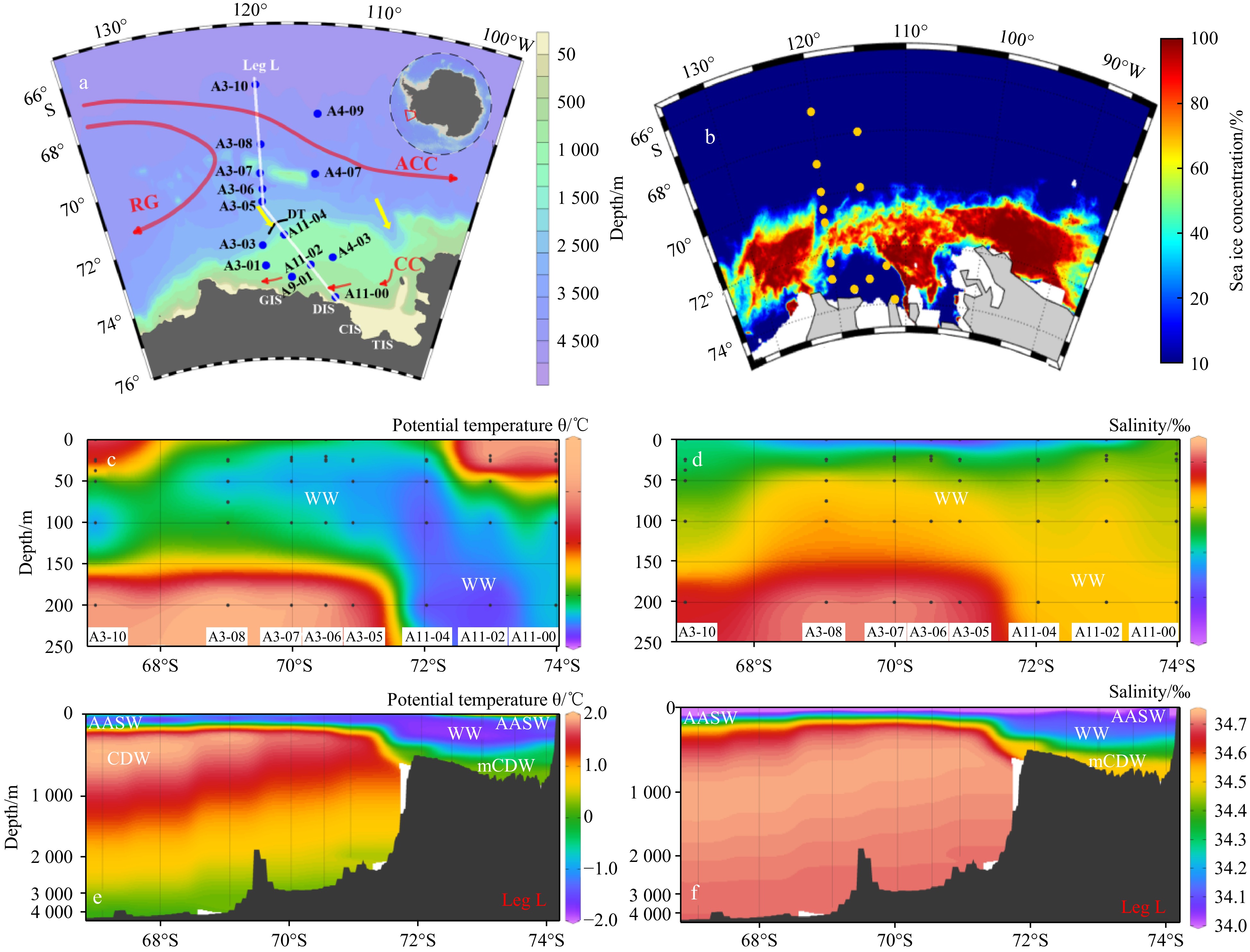
Figure 1. Sampling locations and hydrographic conditions in the Amundsen Sea. a. Study area bathymetry and sampling stations occupied during the 36th Chinese National Antarctic Research Expedition (CHINARE) from January to February 2020. Transect L (Leg L) extends southeastward from the open ocean, traversing the sea ice zone (SIZ) and polynya, to the DIS front. The Dotson Trough (DT) is delineated by a black line at the shelf break. b. Sea ice concentration during the sampling period. c. Vertical profiles of potential temperature (℃) along Transect L (0–250 m). d. Vertical profiles of salinity (‰) along Transect L (0–250 m). e. Vertical profiles of potential temperature (℃) along Transect L (whole water column). f. Vertical profiles of salinity (‰) along Transect L (whole water column). Water masses: AASW: Antarctic Surface Water; WW: Winter Water; mCDW: Modified Circumpolar Deep Water; CDW: Circumpolar Deep Water; ACC: Antarctic Circumpolar Current; RG: Ross Gyre; CC: Coastal current; GIS: Getz Ice Shelf; DIS: Dotson Ice Shelf; CIS: Crosson Ice Shelf; TIS: Thwaites Ice Shelf. The water circulations in Plot a are according to Kim et al. (2017) and Nakayama et al. (2018), red arrows represent water currents, and yellow arrows represent the intrusion of CDW onto the Amundsen Sea shelf.
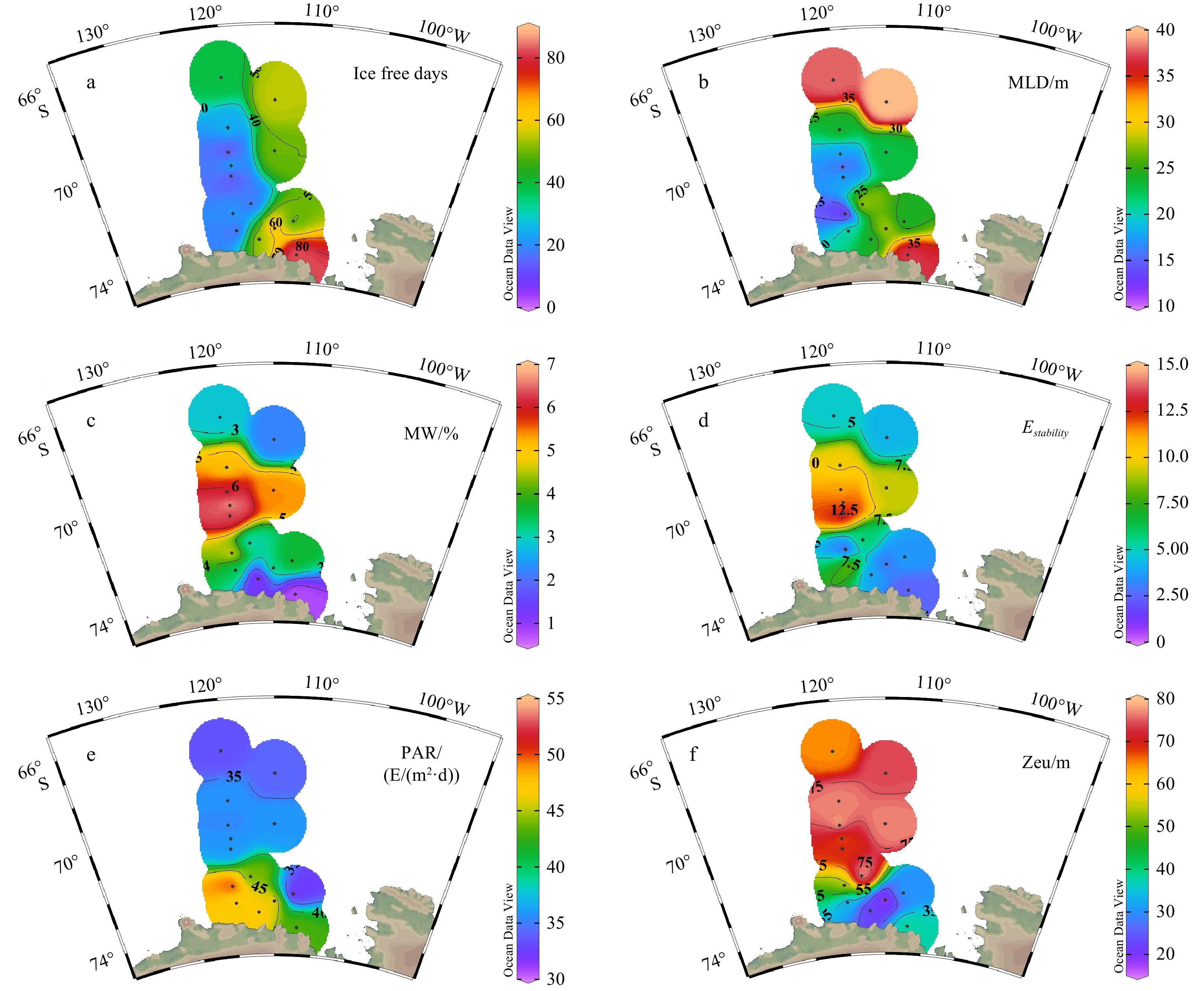
Figure 2. Hydrographic characteristics of the study area: a. Ice-free days (days elapsed between sea ice melting and sampling) b. mixed layer depth (MLD, m); (c. sea ice meltwater fraction (MW%, percentage); d. water column stability (Estability); e. photosynthetically active radiation (PAR); f. Euphotic zone depth (Zeu, m).

Figure 3. Spatial distributions of depth-integrated concentrations (a−c), seasonal utilization (d−f) and utilization ratios (g−i) of nutrients (TN: NO
$ _3^ - $ +NO$ _2^ - $ , silicates and phosphates)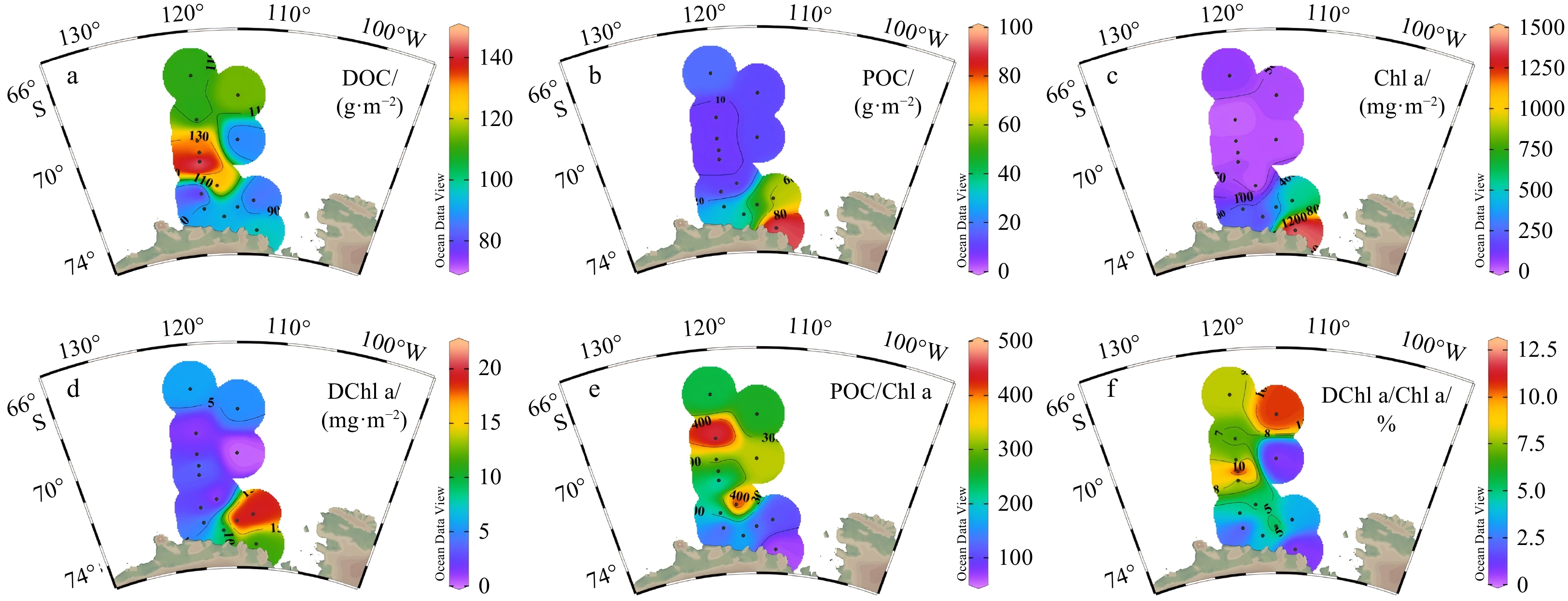
Figure 4. Spatial variations in depth-integrated concentrations of DOC (g/m2) (a), POC (g/m2) (b), Chl a (c), Chl a degradation products (DChl a, mg/m2) (d), POC/Chl a ratio (e), and DChl a/Chl a ratio (f).

Figure 5. Relative abundance of major phytoplankton taxonomic groups and community size structure in the study area. The contribution of Diatoms-A was negligible ( < 1%) and is not shown.
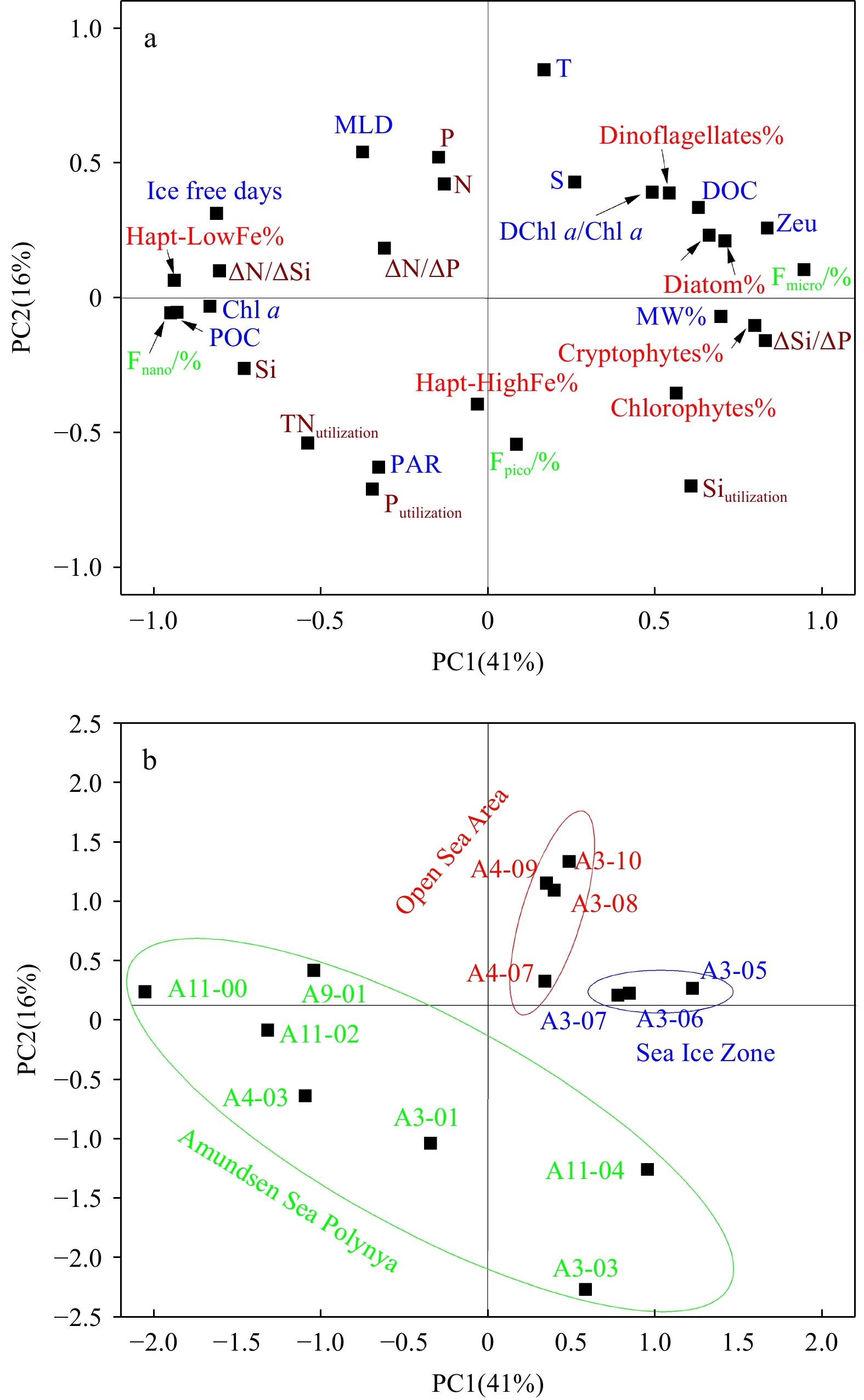
Figure 6. Principal component analysis (PCA) results. a. Variable loadings on Factor1 and Factor 2; b. sample scores on Factor 1 and Factor 2.

Figure 7. Environmental drivers, integrated biogenic substance concentrations and phytoplankton taxonomic compositions along Leg L.
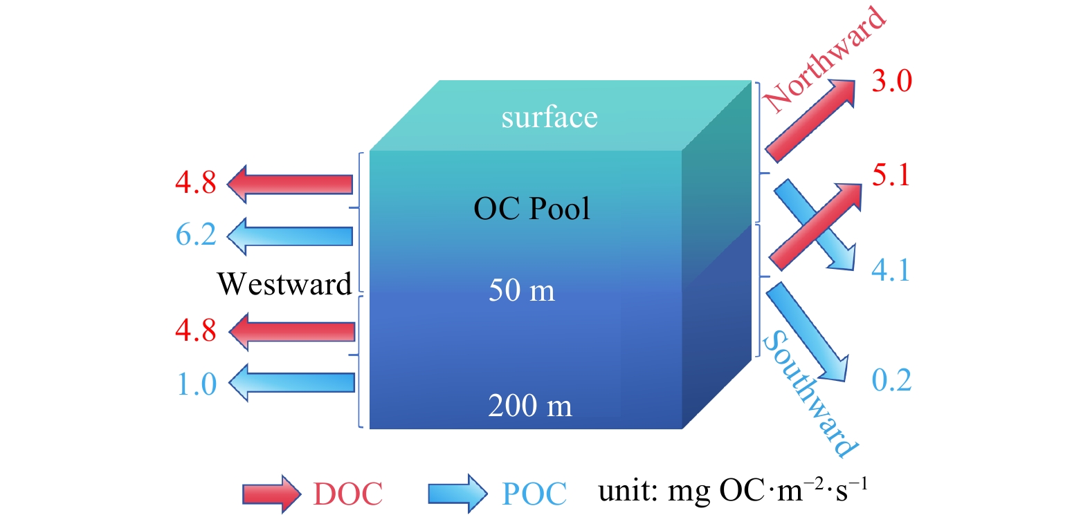
Figure 8. Conceptual model of horizontal OC transport in the ASP. Red arrows represent DOC flux, blue arrows represent POC flux
Table 1. Ratios of concentrations of diagnostic pigments to chlorophyll a (Chl a) used for CHEMTAX analysis
Matrix Chl c3 Peri Fuco Vio Hex-fuco Allo Lutein Chl b Chl a
Initial matrixChlorophytes 0.00 0.00 0.00 0.03 0.00 0.00 0.22 0.18 1.00 Cryptophytes 0.00 0.00 0.00 0.00 0.00 0.22 0.00 0.00 1.00 Diatoms-A 0.00 0.00 0.57 0.00 0.00 0.00 0.00 0.00 1.00 Diatoms-B 0.03 0.00 1.02 0.00 0.00 0.00 0.00 0.00 1.00 Dinoflagellates 0.00 0.54 0.00 0.00 0.00 0.00 0.00 0.00 1.00 Haptophytes (high Fe) 0.13 0.00 0.08 0.00 0.40 0.00 0.00 0.00 1.00 Haptophytes (low Fe) 0.27 0.00 0.02 0.00 1.10 0.00 0.00 0.00 1.00
Final matrixChlorophytes 0.00 0.00 0.00 0.06 0.00 0.00 0.15 0.17 1.00 Cryptophytes 0.00 0.00 0.00 0.00 0.00 0.28 0.00 0.00 1.00 Diatoms-A 0.00 0.00 0.75 0.00 0.00 0.00 0.00 0.00 1.00 Diatoms-B 0.04 0.00 1.08 0.00 0.00 0.00 0.00 0.00 1.00 Dinoflagellates 0.00 0.64 0.00 0.00 0.00 0.00 0.00 0.00 1.00 Haptophytes (high Fe) 0.10 0.00 0.10 0.00 0.43 0.00 0.00 0.00 1.00 Haptophytes (low Fe) 0.21 0.00 0.02 0.00 1.36 0.00 0.00 0.00 1.00 Notes: Initial ratios before analysis (a) and optimized ratios after analysis (b). Chl c3: chlorophyll c3; Peri: peridinin; Hex-fuco: 19’-hexanoyloxyfucoxanthin; Fuco:fucoxanthin; Vio: violaxanthin; Allo: alloxanthin; Chl b: chlorophyll b, and Chl a: chlorophyll a  下载: 导出CSV
-
Ackley S F, Buck K R, Taguchi S. 1979. Standing crop of algae in the sea ice of the Weddell Sea region. Deep-Sea Research Part A. Oceanographic Research Papers, 26(3): 269–281, doi: 10.1016/0198-0149(79)90024-4 Alderkamp A C, Mills M M, van Dijken G L, et al. 2012. Iron from melting glaciers fuels phytoplankton blooms in the Amundsen Sea (Southern Ocean): phytoplankton characteristics and productivity. Deep-Sea Research Part II: Topical Studies in Oceanography, 71–76: 32–48, doi: 10.1016/j.dsr2.2012.03.005 Arrigo K R, Lowry K E, Van Dijken G L, et al. 2012. Annual changes in sea ice and phytoplankton in polynyas of the Amundsen Sea, Antarctica. Deep-Sea Research Part Ⅱ: Topical Studies in Oceanography, 71–76: 5–15, doi: 10.1016/j.dsr2.2012.03.006 Arrigo K R, Robinson D H, Dunbar R B, et al. 2003. Physical control of chlorophyll a, POC, and TPN distributions in the pack ice of the Ross Sea, Antarctica. Journal of Geophysical Research: Oceans, 108(C10): 3316, doi: 10.1029/2001JC001138 Arrigo K R, Sullivan C W. 1992. The influence of salinity and temperature covariation on the photophysiological characteristics of Antarctic sea ice microalgae. Journal of Phycology, 28(6): 746–756, doi: 10.1111/j.0022-3646.1992.00746.x Arrigo K R, van Dijken G L. 2003. Phytoplankton dynamics within 37 Antarctic coastal polynya systems. Journal of Geophysical Research: Oceans, 108(C8): 3271, doi: 10.1029/2002JC001739 Arrigo K R, van Dijken G L, Bushinsky S. 2008. Primary production in the Southern Ocean, 1997–2006. Journal of Geophysical Research: Oceans, 113(C8): C08004, doi: 10.1029/2007JC004551 Arrigo K R, Van Dijken G L, Strong A L. 2015. Environmental controls of marine productivity hot spots around Antarctica. Journal of Geophysical Research: Oceans, 120(8): 5545–5565, doi: 10.1002/2015JC010888 Atkinson A, Hill S L, Barange M, et al. 2014. Sardine cycles, krill declines, and locust plagues: revisiting ‘wasp-waist’ food webs. Trends in Ecology & Evolution, 29(6): 309–316, doi: 10.1016/j.tree.2014.03.011 Bauer J E, Druffel E R M, Wolgast D M, et al. 2001. Sources and cycling of dissolved and particulate organic radiocarbon in the northwest Atlantic continental margin. Global Biogeochemical Cycles, 15(3): 615–636, doi: 10.1029/2000GB001314 Behrenfeld M J, Falkowski P G. 1997. Photosynthetic rates derived from satellite-based chlorophyll concentration. Limnology and Oceanography, 42(1): 1–20, doi: 10.4319/lo.1997.42.1.0001 Belyaev N A, Peresypkin V I, Ponyaev M S. 2010. The organic carbon in the water, the particulate matter, and the upper layer of the bottom sediments of the west Kara Sea. Oceanology, 50(5): 706–715, doi: 10.1134/S0001437010050085 Boyd P W. 2002. Environmental factors controlling phytoplankton processes in the Southern Ocean. Journal of Phycology, 38(5): 844–861, doi: 10.1046/j.1529-8817.2002.t01-1-01203.x Carlson C A, Hansell D A, Peltzer E T, et al. 2000. Stocks and dynamics of dissolved and particulate organic matter in the southern Ross Sea, Antarctica. Deep-Sea Research Part II: Topical Studies in Oceanography, 47(15-16): 3201–3225, doi: 10.1016/S0967-0645(00)00065-5 Carvalho F, Kohut J, Oliver M J, et al. 2016. Mixing and phytoplankton dynamics in a submarine canyon in the west Antarctic Peninsula. Journal of Geophysical Research: Oceans, 121(7): 5069–5083, doi: 10.1002/2016JC011650 Cheah W, Soppa M A, Wiegmann S, et al. 2017. Importance of deep mixing and silicic acid in regulating phytoplankton biomass and community in the iron-limited Antarctic polar front region in summer. Deep-Sea Research Part II: Topical Studies in Oceanography, 138: 74–85, doi: 10.1016/j.dsr2.2016.05.019 Cifuentes L A, Sharp J H, Fogel M L. 1988. Stable carbon and nitrogen isotope biogeochemistry in the Delaware estuary. Limnology and Oceanography, 33(5): 1102–1115, doi: 10.2307/2837243 Costa R R, Mendes C R B, Tavano V M, et al. 2020. Dynamics of an intense diatom bloom in the northern Antarctic Peninsula, February 2016. Limnology and Oceanography, 65(9): 2056–2075, doi: 10.1002/lno.11437 Davidson A T, Scott F J, Nash G V, et al. 2010. Physical and biological control of protistan community composition, distribution and abundance in the seasonal ice zone of the Southern Ocean between 30 and 80°E. Deep-Sea Research Part II: Topical Studies in Oceanography, 57(9–10): 828–848, doi: 10.1016/j.dsr2.2009.02.011 DiTullio G R, Grebmeier J M, Arrigo K R, et al. 2000. Rapid and early export of Phaeocystis antarctica blooms in the Ross Sea, Antarctica. Nature, 404(6778): 595–598, doi: 10.1038/35007061 Ducklow H W, Wilson S E, Post A F, et al. 2015. Particle flux on the continental shelf in the Amundsen Sea polynya and western Antarctic Peninsula. Elementa: Science of the Anthropocene, 3: 000046, doi: 10.12952/journal.elementa.000046 Feng Yubin, Li Dong, Zhao Jun, et al. 2022a. Effects of sea ice melt water input on phytoplankton biomass and community structure in the eastern Amundsen Sea. Advances in Polar Science, 33(1): 14–27, doi: 10.103679/j.advps.2021.0017 Feng Yubin, Li Dong, Zhao Jun, et al. 2022b. Environmental drivers of phytoplankton crops and taxonomic composition in northeastern Antarctic Peninsula adjacent sea area. Acta Oceanologica Sinica, 41(1): 99–117, doi: 10.1007/s13131-021-1865-4 Garrison D L, Buck K R. 1989. Protozooplankton in the Weddell Sea, Antarctica: abundance and distribution in the ice-edge zone. Polar Biology, 9(6): 341–351, doi: 10.1007/BF00442524 Ge Yuncong, Zhang Ruifeng, Zhu Zhuoyi, et al. 2024. Distributions of nutrients, trace metals, phytoplankton composition, and elemental consumption in the Ross and Amundsen Seas. Marine Chemistry, 265–266: 104436, doi: 10.1016/j.marchem.2024.104436 Gibb S W, Cummings D G, Irigoien X, et al. 2001. Phytoplankton pigment chemotaxonomy of the northeastern Atlantic. Deep-Sea Research Part II: Topical Studies in Oceanography, 48(4-5): 795–823, doi: 10.1016/S0967-0645(00)00098-9 Gordon D C, Cranford P J. 1985. Detailed distribution of dissolved and particulate organic matter in the Arctic Ocean and comparison with other oceanic regions. Deep-Sea Research Part A: Oceanographic Research Papers, 32(10): 1221–1232, doi: 10.1016/0198-0149(85)90005-6 Grasshoff K, Kremling K, Ehrhardt M. 1999. Methods of Seawater Analysis. 3rd ed. New York: Wiley-VCH, doi: 10.1002/9783527613984 Griffith D R, Mcnichol A P, Xu L, et al. 2012. Carbon dynamics in the western Arctic Ocean: insights from full-depth carbon isotope profiles of DIC, DOC, and POC. Biogeosciences, 9(3): 1217–1224, doi: 10.5194/bg-9-1217-2012 Gruber N, Clement D, Carter B R, et al. 2019. The oceanic sink for anthropogenic CO2 from 1994 to 2007. Science, 363(6432): 1193–1199, doi: 10.1126/science.aau5153 Ha H K, Wåhlin A K, Kim T W, et al. 2014. Circulation and modification of warm deep water on the central Amundsen Shelf. Journal of Physical Oceanography, 44(5): 1493–1501, doi: 10.1175/JPO-D-13-0240.1 Hassler C S, Ridgway K R, Bowie A R, et al. 2014. Primary productivity induced by iron and nitrogen in the Tasman Sea: an overview of the PINTS expedition. Marine and Freshwater Research, 65(6): 517–537, doi: 10.1071/MF13137 Hopkinson B M, Mitchell B G, Reynolds R A, et al. 2007. Iron limitation across chlorophyll gradients in the southern Drake Passage: phytoplankton responses to iron addition and photosynthetic indicators of iron stress. Limnology and Oceanography, 52(6): 2540–2554, doi: 10.4319/lo.2007.52.6.2540 Hu Ji, Xue Siyou, Zhao Jun, et al. 2023. Dynamics of chromophoric dissolved organic matter in a highly productive Amundsen Sea Polynya. Marine Chemistry, 257: 104329, doi: 10.1016/j.marchem.2023.104329 Hung J J, Lin Paolin, Liu K K. 2000. Dissolved and particulate organic carbon in the southern East China Sea. Continental Shelf Research, 20(4–5): 545–569, doi: 10.1016/S0278-4343(99)00085-0 Hyun J H, Kim S H, Yang E J, et al. 2016. Biomass, production, and control of heterotrophic bacterioplankton during a late phytoplankton bloom in the Amundsen Sea Polynya, Antarctica. Deep-Sea Research Part II: Topical Studies in Oceanography, 123: 102–112, doi: 10.1016/j.dsr2.2015.10.001 Jarvis T, Kelly N, Kawaguchi S, et al. 2010. Acoustic characterisation of the broad-scale distribution and abundance of Antarctic krill (Euphausia superba) off east Antarctica (30–80°E) in January–March 2006. Deep-Sea Research Part II: Topical Studies in Oceanography, 57(9-10): 916–933, doi: 10.1016/j.dsr2.2008.06.013 Jenkins A, Dutrieux P, Jacobs S, et al. 2016. Decadal ocean forcing and Antarctic Ice Sheet response: lessons from the Amundsen sea. Oceanography, 29(4): 106–117, doi: 10.5670/oceanog.2016.103 Joy-Warren H L, Van Dijken G L, Alderkamp A C, et al. 2019. Light is the primary driver of early season phytoplankton production along the western Antarctic Peninsula. Journal of Geophysical Research: Oceans, 124(11): 7375–7399, doi: 10.1029/2019jc015295 Kim T W, Ha H K, Wåhlin A K, et al. 2017. Is Ekman pumping responsible for the seasonal variation of warm circumpolar deep water in the Amundsen Sea? Continental Shelf Research, 132: 38–48, doi: 10.1016/j.csr.2016.09.005 Kim M, Hwang J, Lee S H, et al. 2016. Sedimentation of particulate organic carbon on the Amundsen Shelf, Antarctica. Deep-Sea Research Part II: Topical Studies in Oceanography, 123: 135–144, doi: 10.1016/j.dsr2.2015.07.018 Kim M, Yang E J, Kim H J, et al. 2019. Collection of large benthic invertebrates in sediment traps in the Amundsen Sea, Antarctica. Biogeosciences, 16(13): 2683–2691, doi: 10.5194/bg-16-2683-2019 Kropuenske L R, Mills M M, van Dijken G L, et al. 2010. Strategies and rates of photoacclimation in two major southern ocean phytoplankton taxa: Phaeocystis antarctica (haptophyta) and Fragilariopsis cylindrus (bacillariophyceae). Journal of Phycology, 46(6): 1138–1151, doi: 10.1111/j.1529-8817.2010.00922.x Lannuzel D, Chever F, van der Merwe P C, et al. 2016. Iron biogeochemistry in Antarctic pack ice during SIPEX-2. Deep-Sea Research Part II: Topical Studies in Oceanography, 131: 111–122, doi: 10.1016/j.dsr2.2014.12.003 Lee S, Hwang J, Ducklow H W, et al. 2017. Evidence of minimal carbon sequestration in the productive Amundsen Sea Polynya. Geophysical Research Letters, 44(15): 7892–7899, doi: 10.1002/2017gl074646 Lee Y, Yang E J, Park J, et al. 2016. Physical-biological coupling in the Amundsen Sea, Antarctica: influence of physical factors on phytoplankton community structure and biomass. Deep-Sea Research Part I: Oceanographic Research Papers, 117: 51–60, doi: 10.1016/j.dsr.2016.10.001 Li Yuhong, Zhao Jun, Li Dong, et al. 2024. Factors controlling the phytoplankton crops, taxonomic composition, and particulate organic carbon stocks in the Cosmonaut Sea, East Antarctica. Journal of Oceanology and Limnology, 42(6): 1895–1908, doi: 10.1007/s00343-024-3198-6 Long M C, Stephens B B, Mckain K, et al. 2021. Strong Southern Ocean carbon uptake evident in airborne observations. Science, 374(6572): 1275–1280, doi: 10.1126/science.abi4355 Meijers A J S, Klocker A, Bindoff N L, et al. 2010. The circulation and water masses of the Antarctic shelf and continental slope between 30 and 80°E. Deep-Sea Research Part II: Topical Studies in Oceanography, 57(9-10): 723–737, doi: 10.1016/j.dsr2.2009.04.019 Mendes C R B, Tavano V M, Dotto T S, et al. 2018a. New insights on the dominance of cryptophytes in Antarctic coastal waters: a case study in Gerlache Strait. Deep-Sea Research Part II: Topical Studies in Oceanography, 149: 161–170, doi: 10.1016/j.dsr2.2017.02.010 Mendes C R B, Tavano V M, Kerr R, et al. 2018b. Impact of sea ice on the structure of phytoplankton communities in the northern Antarctic Peninsula. Deep-Sea Research Part II: Topical Studies in Oceanography, 149: 111–123, doi: 10.1016/j.dsr2.2017.12.003 Mendes C R B, Tavano V M, Leal M C, et al. 2013. Shifts in the dominance between diatoms and cryptophytes during three late summers in the Bransfield Strait (Antarctic Peninsula). Polar Biology, 36(4): 537–547, doi: 10.1007/s00300-012-1282-4 Morel A, Huot Y, Gentili B, et al. 2007. Examining the consistency of products derived from various ocean color sensors in open ocean (case 1) waters in the perspective of a multi-sensor approach. Remote Sensing of Environment, 111(1): 69–88, doi: 10.1016/j.rse.2007.03.012 Nakatsuka T, Toda M, Kawamura K, et al. 2004. Dissolved and particulate organic carbon in the Sea of Okhotsk: transport from continental shelf to ocean interior. Journal of Geophysical Research: Oceans, 109(C9): C09S14, doi: 10.1029/2003JC001909 Nakayama Y, Menemenlis D, Zhang H, et al. 2018. Origin of circumpolar deep water intruding onto the Amundsen and Bellingshausen Sea continental shelves. Nature Communications, 9(1): 3403, doi: 10.1038/s41467-018-05813-1 Nakayama Y, Schröder M, Hellmer H H, 2013. From circumpolar deep water to the glacial meltwater plume on the eastern Amundsen Shelf. Deep-Sea Research Part I: Oceanographic Research Papers, 77, 50–62, doi: 10.1016/j.dsr.2013.04.001 Nomura D, Aoki S, Simizu D, et al. 2018. Influence of sea ice crack formation on the spatial distribution of nutrients and microalgae in flooded Antarctic multiyear ice. Journal of Geophysical Research: Oceans, 123(2): 939–951, doi: 10.1002/2017JC012941 Oliver H, St-Laurent P, Sherrell R M, et al. 2019. Modeling iron and light controls on the summer Phaeocystis antarctica bloom in the Amundsen Sea Polynya. Global Biogeochemical Cycles, 33(5): 570–596, doi: 10.1029/2018GB006168 Park Y H, Charriaud E, Craneguy P, et al. 2001. Fronts, transport, and Weddell gyre at 30°E between Africa and Antarctica. Journal of Geophysical Research: Oceans, 106(C2): 2857–2879, doi: 10.1029/2000JC900087 Park J, Kuzminov F I, Bailleul B, et al. 2017. Light availability rather than Fe controls the magnitude of massive phytoplankton bloom in the Amundsen Sea Polynyas, Antarctica. Limnology and Oceanography, 62(5): 2260–2276, doi: 10.1002/lno.10565 Park K, Hahm D, Choi J O, et al. 2019. Spatiotemporal variation in summer net community production in the Amundsen Sea polynya: A self-organizing map analysis approach. Continental Shelf Research, 184: 21–29, doi: 10.1016/j.csr.2019.07.001 Peeken I. 1997. Photosynthetic pigment fingerprints as indicators of phytoplankton biomass and development in different water masses of the Southern Ocean during austral spring. Deep-Sea Research Part II: Topical Studies in Oceanography, 44(1–2): 261–282, doi: 10.1016/s0967-0645(96)00077-x Petty A A, Feltham D L, Holland P R. 2013. Impact of atmospheric forcing on Antarctic continental shelf water masses. Journal of Physical Oceanography, 43(5): 920–940, doi: 10.1175/JPO-D-12-0172.1 Pritchard H D, Ligtenberg S R M, Fricker H A, et al. 2012. Antarctic ice-sheet loss driven by basal melting of ice shelves. Nature, 484(7395): 502–505, doi: 10.1038/nature10968 Randall-Goodwin E, Meredith M P, Jenkins A, et al. 2015. Freshwater distributions and water mass structure in the Amundsen Sea Polynya region, Antarctica. Elementa: Science of the Anthropocene, 3: 000065, doi: 10.12952/journal.elementa.000065 Reigstad M, Wassmann P. 2007. Does Phaeocystis spp. contribute significantly to vertical export of organic carbon?. In: Leeuwe M A, Stefels J, Belviso S, et al, eds. Phaeocystis, Major Link in the Biogeochemical Cycling of Climate-Relevant Elements. Dordrecht: Springer, 217–234, doi: 10.1007/978-1-4020-6214-8_16 Rignot E, Jacobs S, Mouginot J, et al. 2013. Ice-shelf melting around Antarctica. Science, 341(6143): 266–270, doi: 10.1126/science.1235798 Rubin S I, Takahashi T, Chipman D W, et al. 1998. Primary productivity and nutrient utilization ratios in the pacific sector of the Southern Ocean based on seasonal changes in seawater chemistry. Deep-Sea Research Part I: Oceanographic Research Papers, 45(8): 1211–1234, doi: 10.1016/s0967-0637(98)00021-1 Russo A D P G, de Souza M S, Mendes C R B, et al. 2018. Spatial variability of photophysiology and primary production rates of the phytoplankton communities across the western Antarctic Peninsula in late summer 2013. Deep-Sea Research Part II: Topical Studies in Oceanography, 149: 99–110, doi: 10.1016/j.dsr2.2017.09.021 Schoof C, 2010. Ice-sheet acceleration driven by melt supply variability. Nature, 468, 803–806, doi: 10.1038/nature09618 Sherrell R M, Lagerström M E, Forsch K O, et al. 2015. Dynamics of dissolved iron and other bioactive trace metals (Mn, Ni, Cu, Zn) in the Amundsen Sea polynya, Antarctica. Elementa: Science of the Anthropocene, 3: 000071, doi: 10.12952/journal.elementa.000071 Smith W O Jr, Ainley D G, Arrigo K R, et al. 2014. The oceanography and ecology of the Ross Sea. Annual Review of Marine Science, 6: 469–487, doi: 10.1146/annurev-marine-010213-135114 Smith W O Jr, Carlson C A, Ducklow H W, et al. 1998. Growth dynamics of Phaeocystis antarctica-dominated plankton assemblages from the Ross Sea. Marine Ecology Progress Series, 168: 229–244, doi: 10.3354/meps168229 St-Laurent P, Yager P L, Sherrell R M, et al. 2017. Pathways and supply of dissolved iron in the Amundsen Sea (Antarctica). Journal of Geophysical Research: Oceans, 122(9): 7135–7162, doi: 10.1002/2017JC013162 Swalethorp R, Dinasquet J, Logares R, et al. 2019. Microzooplankton distribution in the Amundsen Sea Polynya (Antarctica) during an extensive Phaeocystis antarctica bloom. Progress in Oceanography, 170: 1–10, doi: 10.1016/j.pocean.2018.10.008 Sweeney C, Hansell D A, Carlson C A, et al. 2000. Biogeochemical regimes, net community production and carbon export in the Ross Sea, Antarctica. Deep-Sea Research Part II: Topical Studies in Oceanography, 47(15–16): 3369–3394, doi: 10.1016/S0967-0645(00)00072-2 Takahashi T, Sutherland S C, Wanninkhof R, et al. 2009. Climatological mean and decadal change in surface ocean pCO2, and net sea–air CO2 flux over the global oceans. Deep-Sea Research Part II: Topical Studies in Oceanography, 56(8–10): 554–577, doi: 10.1016/j.dsr2.2008.12.009 Turner J T. 2015. Zooplankton fecal pellets, marine snow, phytodetritus and the ocean’s biological pump. Progress in Oceanography, 130: 205–248, doi: 10.1016/j.pocean.2014.08.005 Uitz J, Claustre H, Griffiths F B, et al. 2009. A phytoplankton class-specific primary production model applied to the Kerguelen Islands region (Southern Ocean). Deep-Sea Research Part I: Oceanographic Research Papers, 56(4): 541–560, doi: 10.1016/j.dsr.2008.11.006 Uitz J, Claustre H, Morel A, et al. 2006. Vertical distribution of phytoplankton communities in open ocean: an assessment based on surface chlorophyll. Journal of Geophysical Research: Oceans, 111(C8): CO8005, doi: 10.1029/2005jc003207 Van Manen M, Aoki S, Brussaard C P D, et al. 2022. The role of the Dotson ice shelf and circumpolar deep water as driver and source of dissolved and particulate iron and manganese in the Amundsen Sea polynya, Southern Ocean. Marine chemistry, 246: 104161, doi: 10.1016/j.marchem.2022.104161 Vidussi F, Claustre H, Manca B B, et al. 2001. Phytoplankton pigment distribution in relation to upper thermocline circulation in the eastern Mediterranean Sea during winter. Journal of Geophysical Research: Oceans, 106(C9): 19939–19956, doi: 10.1029/1999JC000308 Wåhlin A K, Kalén O, Assmann K M, et al. 2016. Subinertial oscillations on the Amundsen Sea Shelf, Antarctica. Journal of Physical Oceanography, 46(9): 2573–2582, doi: 10.1175/JPO-D-14-0257.1 Weston K, Jickells T D, Carson D S, et al. 2013. Primary production export flux in Marguerite Bay (Antarctic Peninsula): linking upper water-column production to sediment trap flux. Deep-Sea Research Part I: Oceanographic Research Papers, 75: 52–66, doi: 10.1016/j.dsr.2013.02.001 Williams G D, Nicol S, Aoki S, et al. 2010. Surface oceanography of BROKE-west, along the Antarctic margin of the south-west Indian Ocean (30–80°E). Deep-Sea Research Part II: Topical Studies in Oceanography, 57(9–10): 738–757, doi: 10.1016/j.dsr2.2009.04.020 Wojtasiewicz B, Trull T W, Clementson L, et al. 2019. Factors controlling the lack of phytoplankton biomass in naturally iron fertilized waters near heard and McDonald islands in the Southern Ocean. Frontiers in Marine Science, 6: 531, doi: 10.3389/fmars.2019.00531 Wright S W, Ishikawa A, Marchant H J, et al. 2009. Composition and significance of picophytoplankton in Antarctic waters. Polar Biology, 32(5): 797–808, doi: 10.1007/s00300-009-0582-9 Wright S W, van den Enden R L, Pearce I, et al. 2010. Phytoplankton community structure and stocks in the Southern Ocean (30–80°E) determined by CHEMTAX analysis of HPLC pigment signatures. Deep-Sea Research Part II: Topical Studies in Oceanography, 57(9–10): 758–778, doi: 10.1016/j.dsr2.2009.06.015 Xue Siyou, Hu Ji, Feng Yubin, et al. 2022. Distribution of transparent exopolymer particles and their response to phytoplankton community structure changes in the Amundsen Sea, Antarctica. Advances in Polar Science, 33(1): 44–54, doi: 10.13679/j.advps.2021.0034 Yager P L, Sherrell R M, Stammerjohn S E, et al. 2016. A carbon budget for the Amundsen Sea Polynya, Antarctica: estimating net community production and export in a highly productive polar ecosystem. Elementa: Science of the Anthropocene, 4: 000140, doi: 10.12952/journal.elementa.000140 Yang Guang, Han Zengbing, Pan Jianming, et al. 2019. Contribution of zooplankton faecal pellets to carbon transport of the mesopelagic layers in the polynya region of Prydz Bay, Antarctica. Estuarine, Coastal and Shelf Science, 222: 139–146, doi: 10.1016/j.ecss.2019.04.006 Yu Peisong, Li Dong, Zhao Jun, et al. 2024. Organic carbon cycling in the sediments of Prydz Bay, eastern Antarctica: implications for a high carbon sequestration potential. Science of the Total Environment, 952: 175894, doi: 10.1016/j.scitotenv.2024.175894 Zamanillo M, Ortega-Retuerta E, Nunes S, et al. 2019. Distribution of transparent exopolymer particles (TEP) in distinct regions of the Southern Ocean. Science of the Total Environment, 691: 736–748, doi: 10.1016/j.scitotenv.2019.06.524 Zapata M, Rodríguez F, Garrido J. 2000. Separation of chlorophylls and carotenoids from marine phytoplankton: a new HPLC method using a reversed phase C8 column and pyridine-containing mobile phases. Marine Ecology Progress Series, 195: 29–45, doi: 10.3354/meps195029 Zhuang Yanpei, Jin Haiyan, Li Hongliang, et al. 2014. Phytoplankton composition and its ecological effect in subsurface cold pool of the northern Bering Sea in summer as revealed by HPLC derived pigment signatures. Acta Oceanologica Sinica, 33(6): 103–111, doi: 10.1007/s13131-014-0495-5 Zu Yongcan, Gao Libao, Guo Guijun, et al. 2022. Changes of circumpolar deep water between 2006 and 2020 in the south-west Indian Ocean, east Antarctica. Deep-Sea Research Part II: Topical Studies in Oceanography, 197: 105043, doi: 10.1016/j.dsr2.2022.105043 -

 DownLoad:


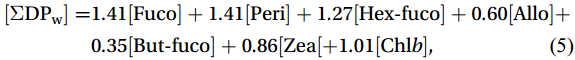


 点击查看大图
计量
- 文章访问数: 37
- HTML全文浏览量: 14
- 被引次数: 0

