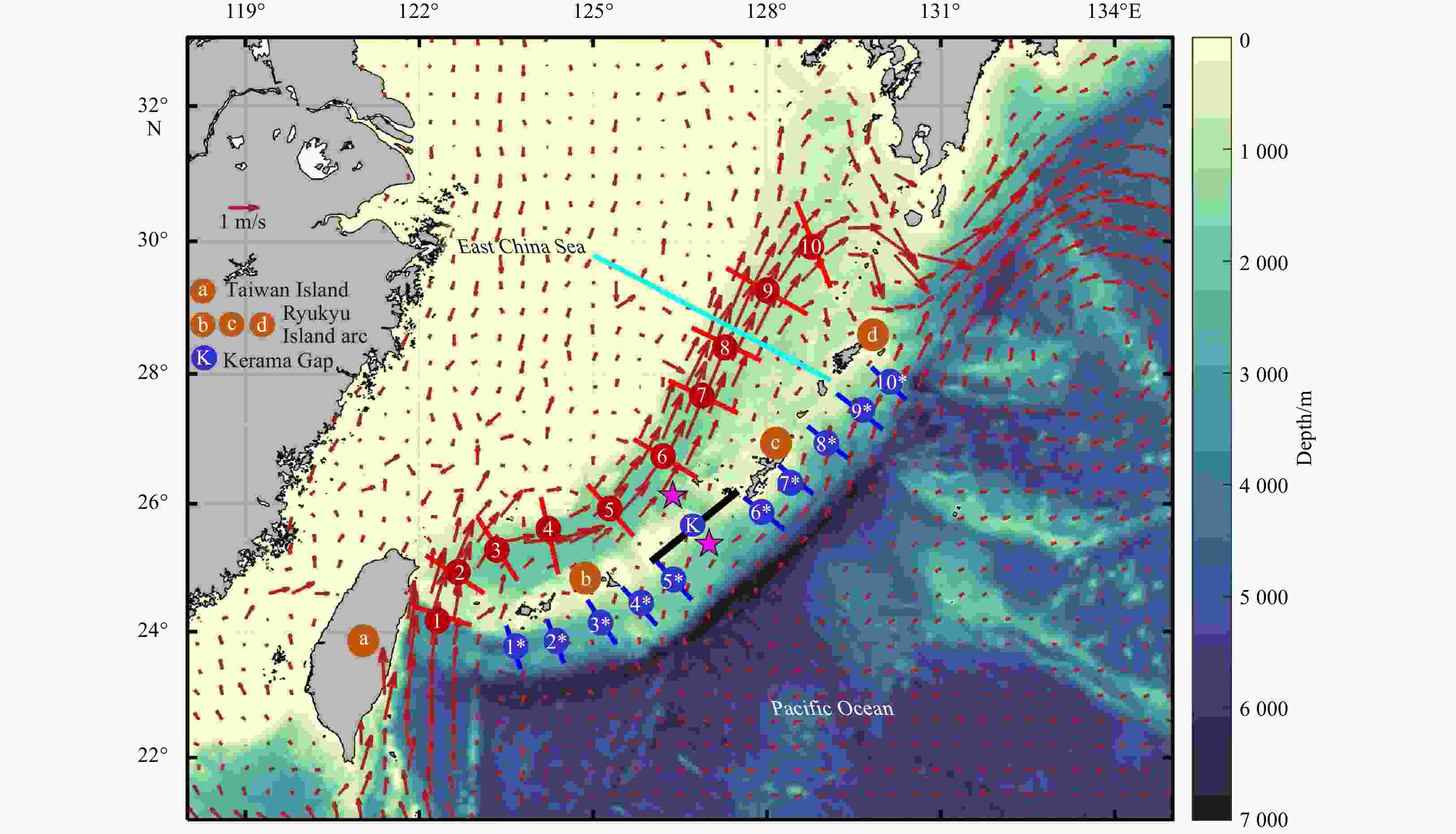
Figure  1.  Geographic location and bathymetry of the study area. Vectors represent the climatological mean (1950–2017) surface current field from the OGCM for the Earth Simulator (OFES). The shaded background color represents the water depth (unit: m, the water depth in the yellow area is very shallow). The black line indicates the location of the Kerama Gap. Two pink stars indicate the positions of the vertical potential density profiles on the both sides of the Kerama Gap, which are shown in Fig. 2. Ten red (blue) lines represent ten sections of the ECS-Kuroshio (Ryukyu) Current, while the cyan line denotes the location of the PN section.

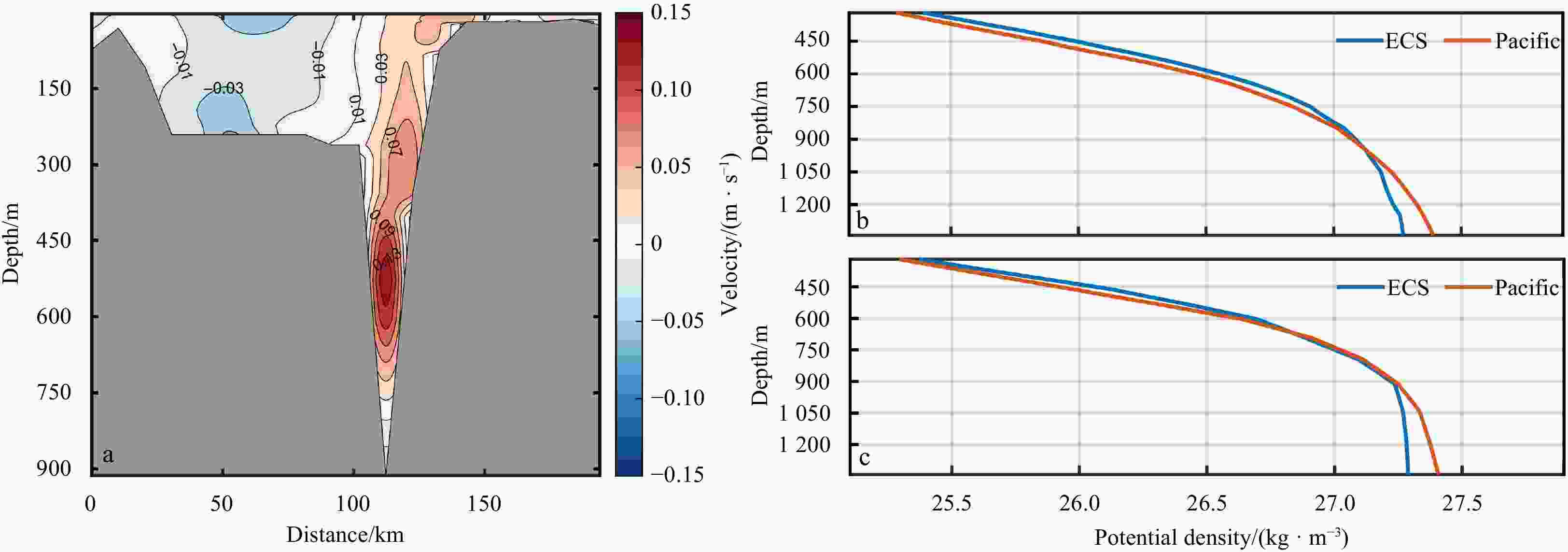
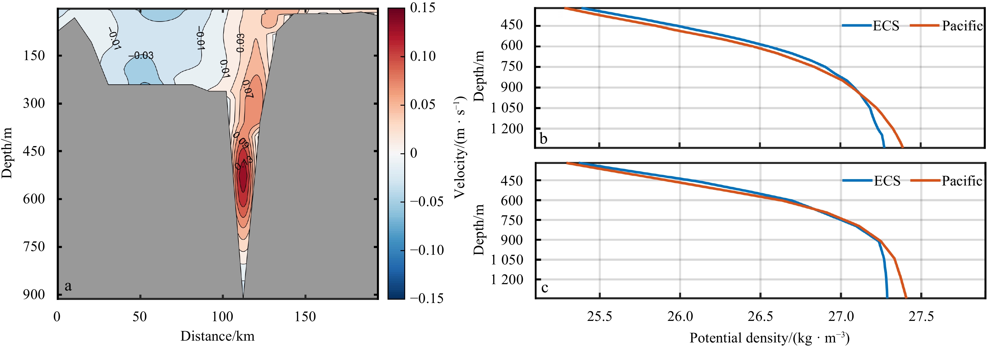
Figure  2.  Vertical section of the long-term mean velocity (unit: m/s) through the Kerama Gap derived from OFES (a), and a comparison of two long-term mean (1955–2017) vertical potential density profiles on both sides of the Kerama Gap derived from WOA 18 (b) and derived from OFES (c). In a, positive values indicate the flow towards the Pacific Ocean, and distance was measured from the southwestern end of the section depicted in Fig. 1. For b and c, the locations are shown in Fig. 1 (two pink stars), and the red (blue) lines represent the profiles on the Pacific (ECS) side.

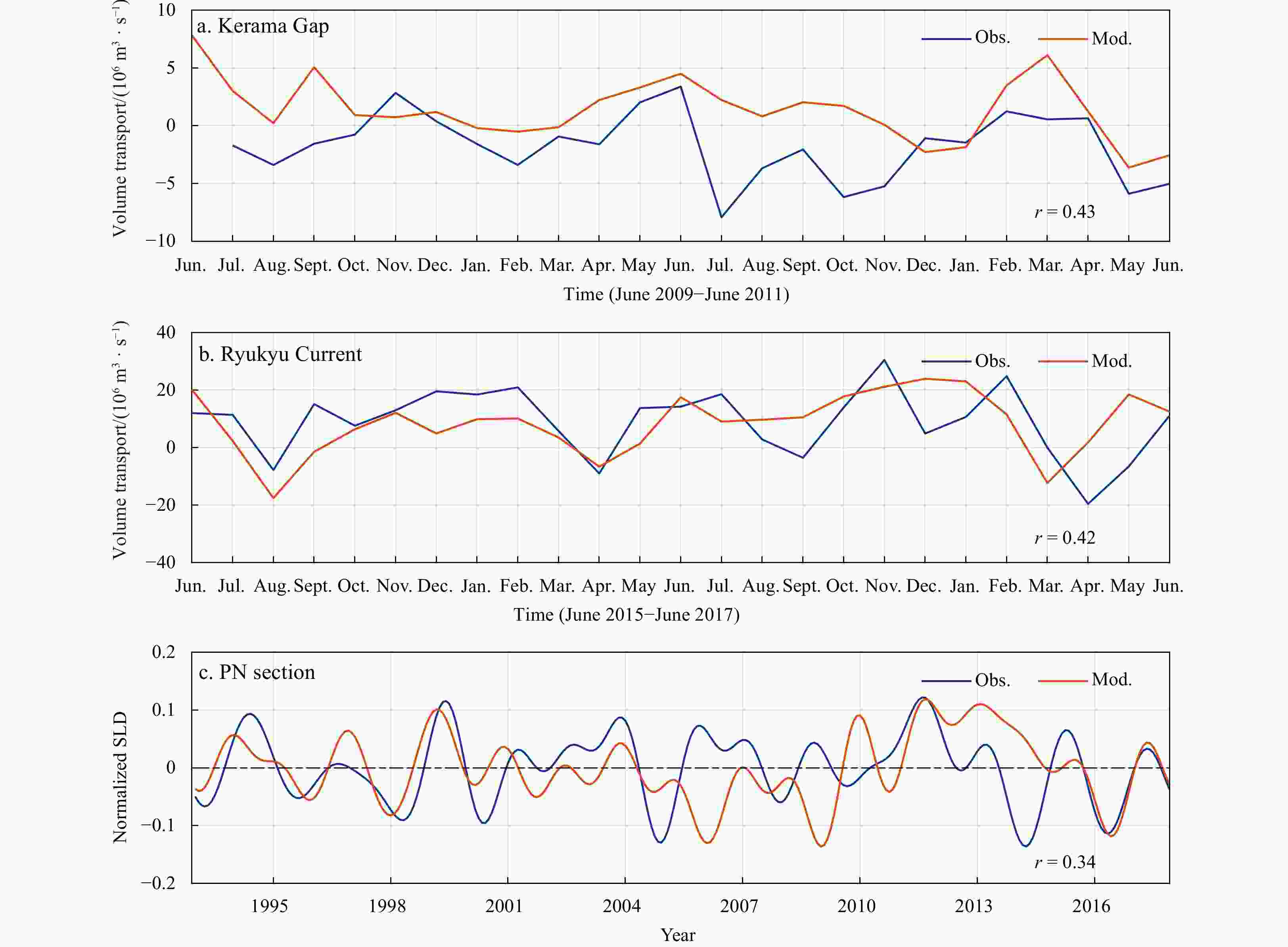
Figure  3.  Comparison of the transport between the observations (Obs., blue) and the model (Mod., red) (a and b) and normalized sea level difference (SLD) for the PN section (c) . a. Two-year KGT from June 2009 to June 2011, and the observational time series is from Na et al. (2014). b. Two-year Ryukyu Current transport from June 2015 to June 2017, and the observational time series is from Zhao et al. (2020).

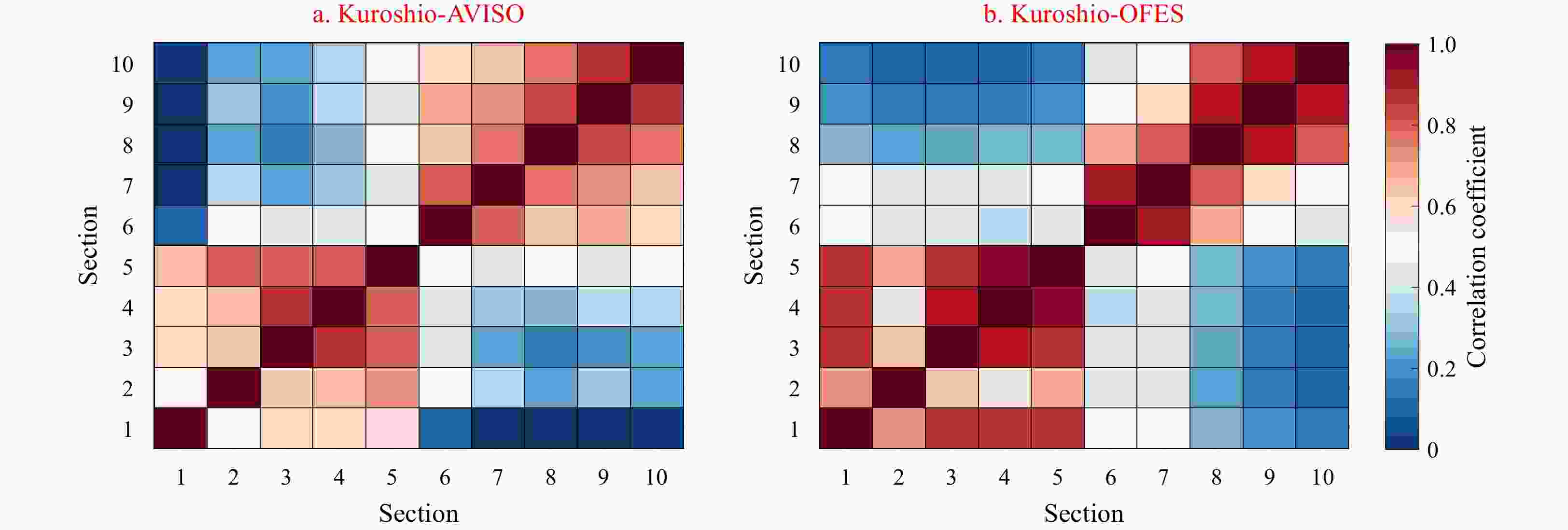
Figure  4.  Correlogram of the interannual variability of the surface geostrophic transport for the ten Kuroshio sections estimated from AVISO data (a) and OFES output (b) during 1993 to 2017, respectively.

Figure  5.  Correlogram of the interannual variability of the vertical integrated volume transport for the ten sections of Kuroshio (a) and Ryukyu Current (b) estimated from the OFES outputs during 1993 to 2017, respectively.

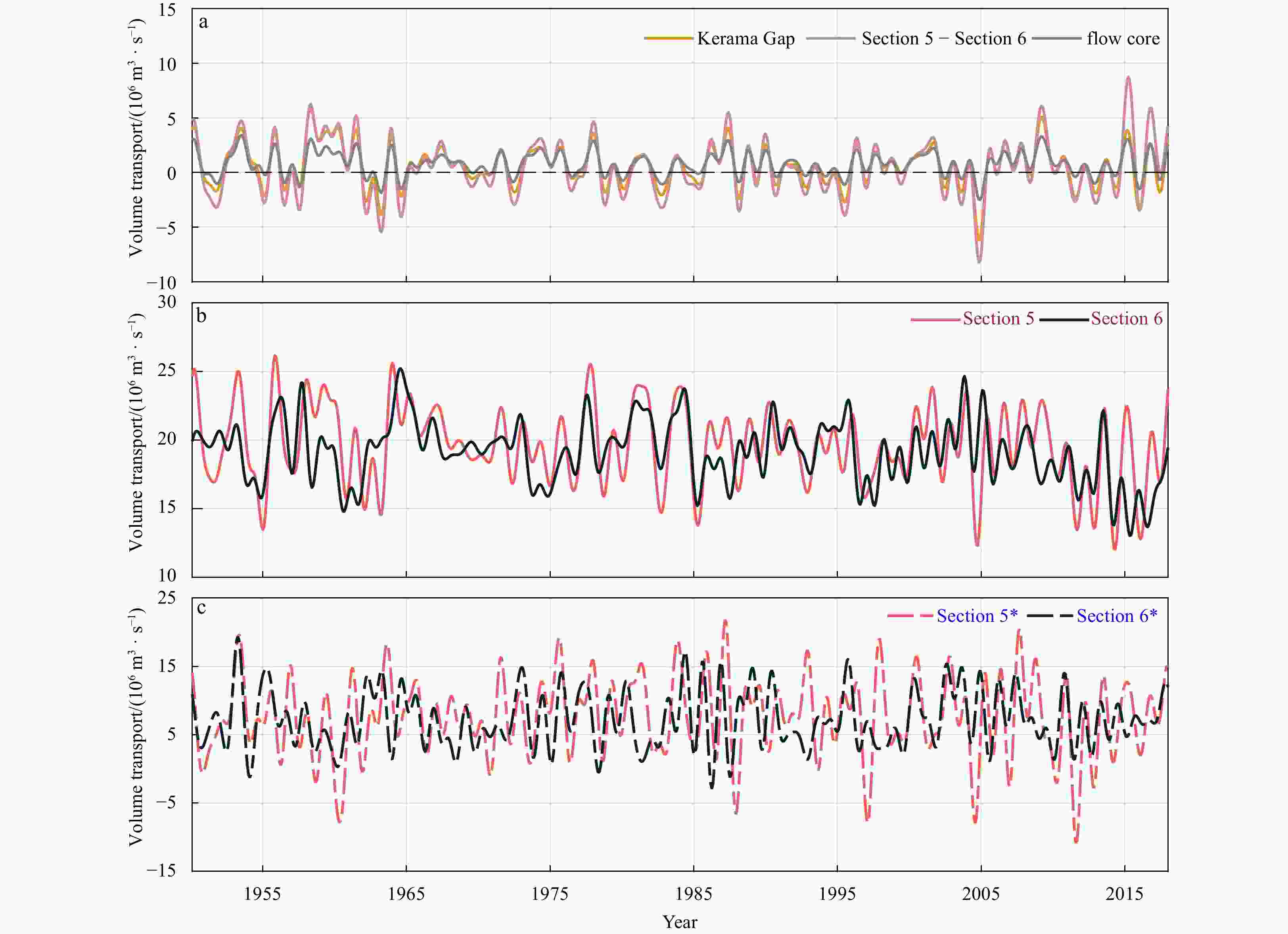
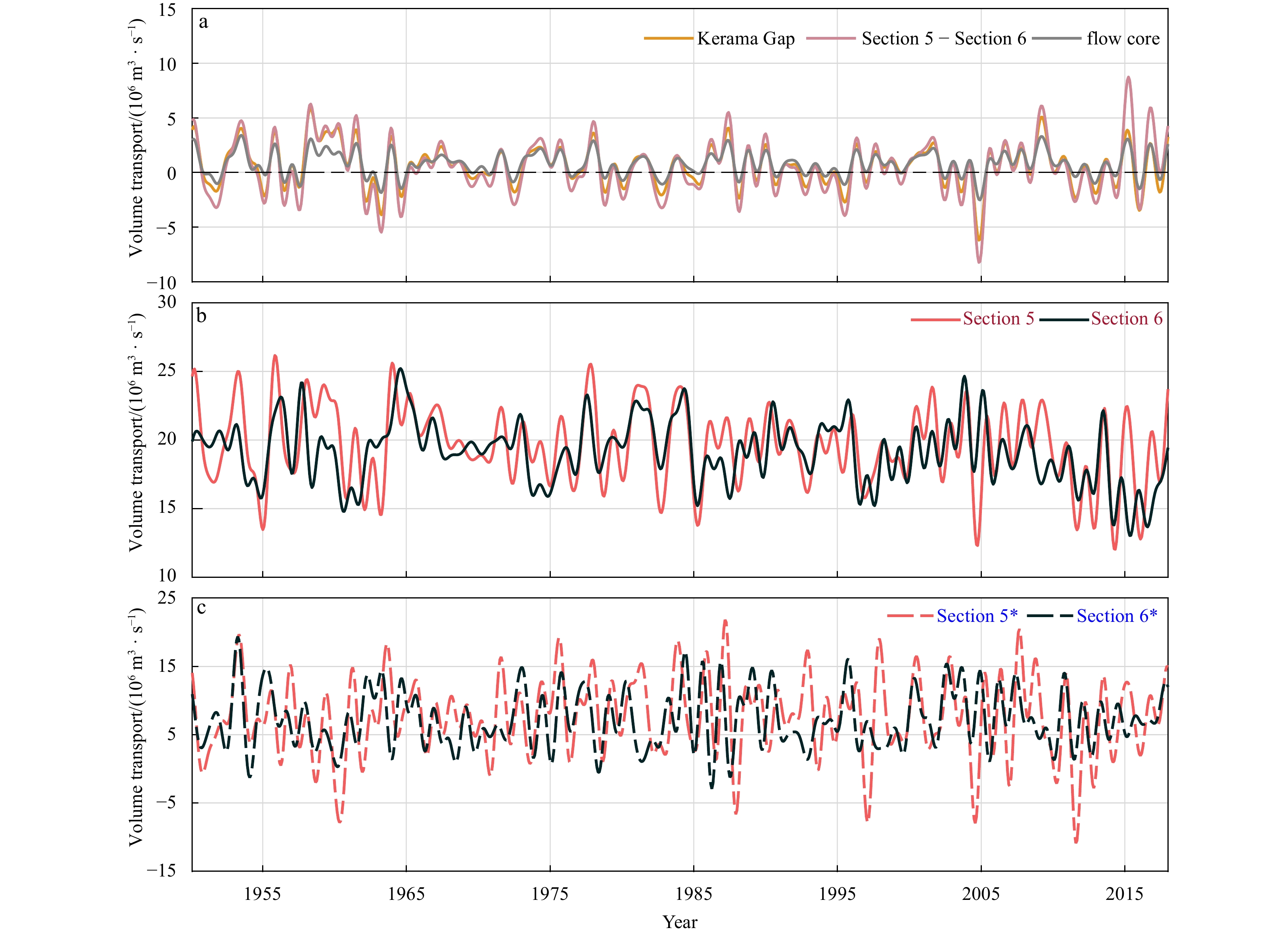
Figure  6.  The interannual variability of the volume transport through the Kerama Gap (eastward is positive) and the difference between the Section 5 and Section 6 of the ECS-Kuroshio (red) (a), the interannual variability of the volume transport through Section 5 (upstream) and Section 6 (downstream) of the ECS-Kuroshio (northward is positive) (b), and the interannual variability of the volume transport through Section 5* (upstream) and Section 6* (downstream) of the Ryukyu Current (northward is positive) (c) during 1950–2017. In a, the gray line represents the volume transport of the deep flow core between 400 m and 700 m.

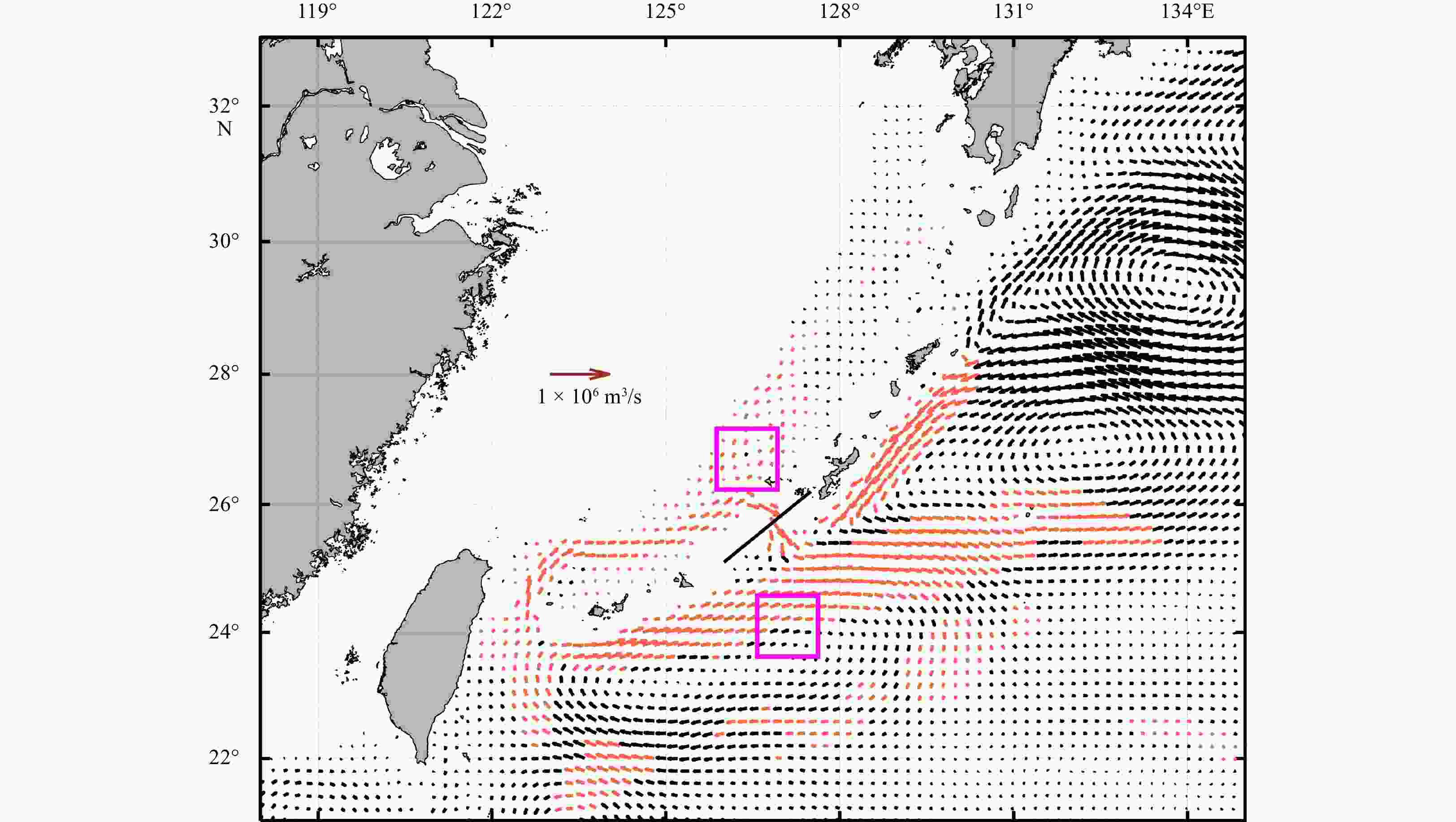
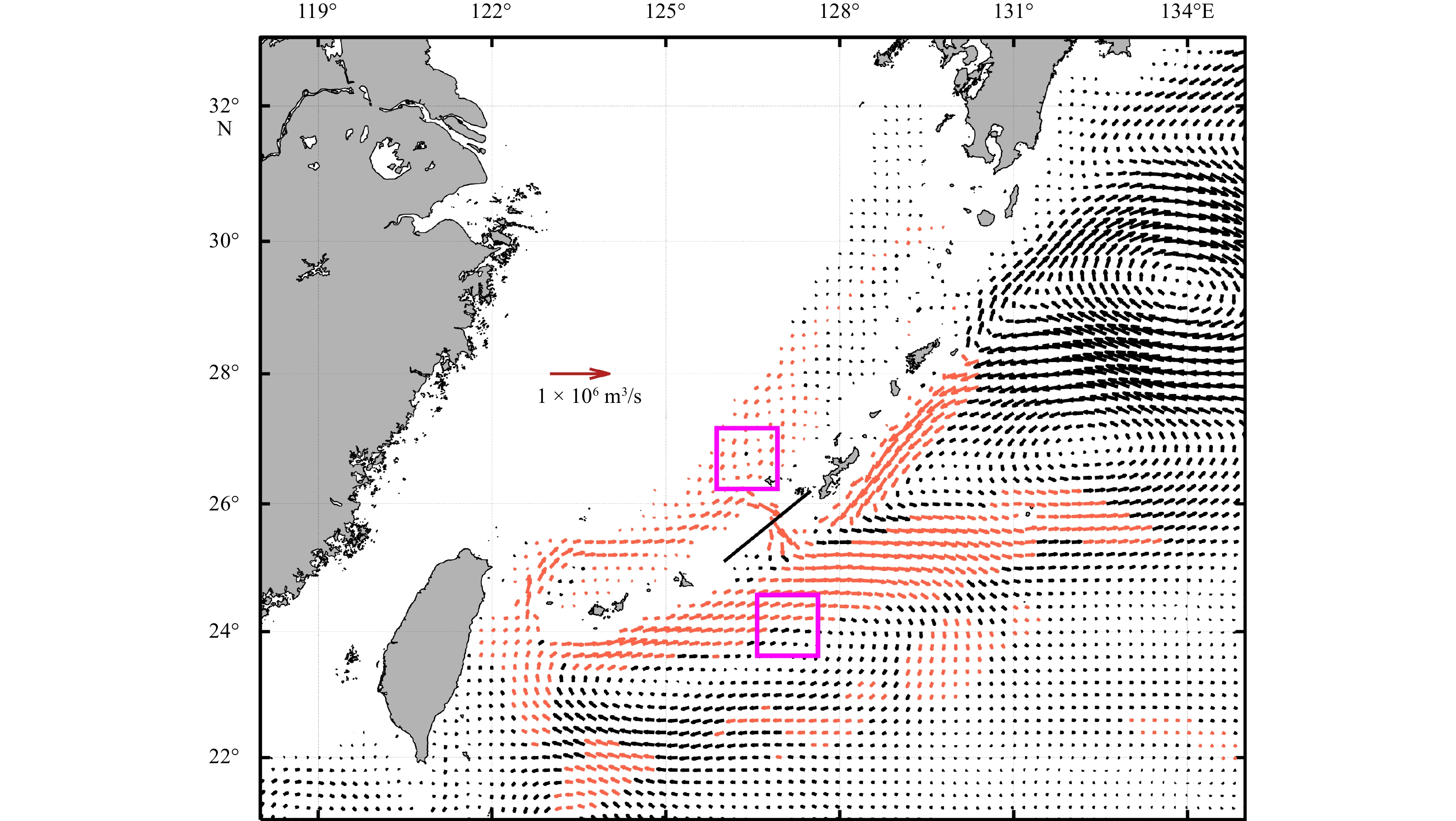
Figure  7.  Composite analysis of the vertical integrated volume transport (unit: 10⁶ m³/s) for the Kuroshio/Ryukyu Current system using the difference between the positive and negative phase of the KGT (Fig. 6a). Red vectors represent the local transport exceeding the 99% significant level. The two 1° × 1° boxes indicate the region for the calculation of the $ \Delta \eta $ and $ \Delta h $. The centers of the ECS and Pacific regions are 26.7°N, 126.4°E and 24.1°N, 127.1°E, respectively.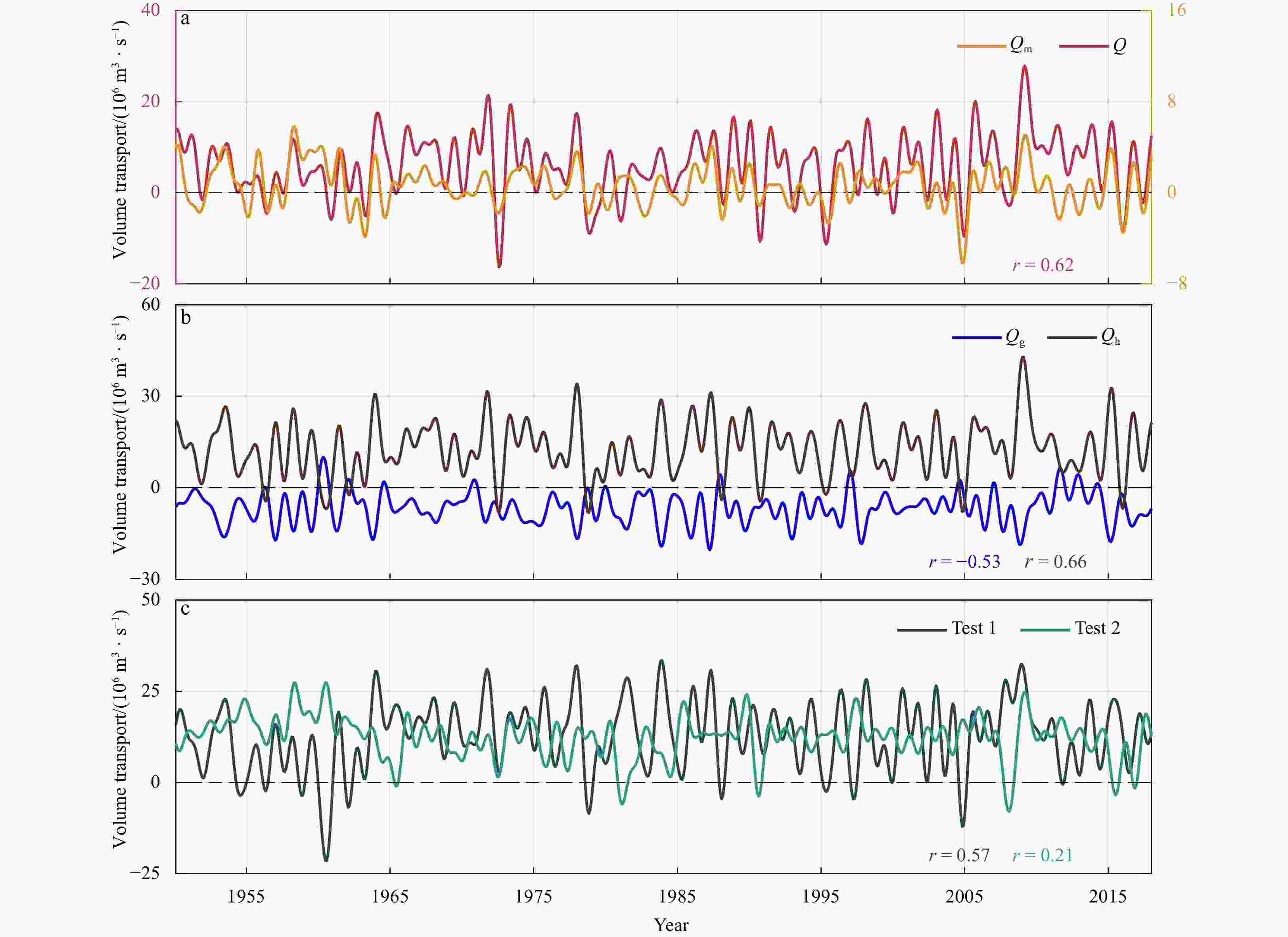

Figure  8.  Comparison of the interannual variability of Q_m (orange) and Q (red) (a), comparison of the interannual variability of Q_g (blue) and Q_h (brown) (b), and two sensitivity test results including holding h_u constant (Test 1; dark green) and holding h_d constant (Test 2; light green) (c). For a, the correlation coefficient is shown at the bottom; for b and c, the correlation coefficients between the two series and Q_m and between the two tests and Q_m are shown at the bottom, respectively.

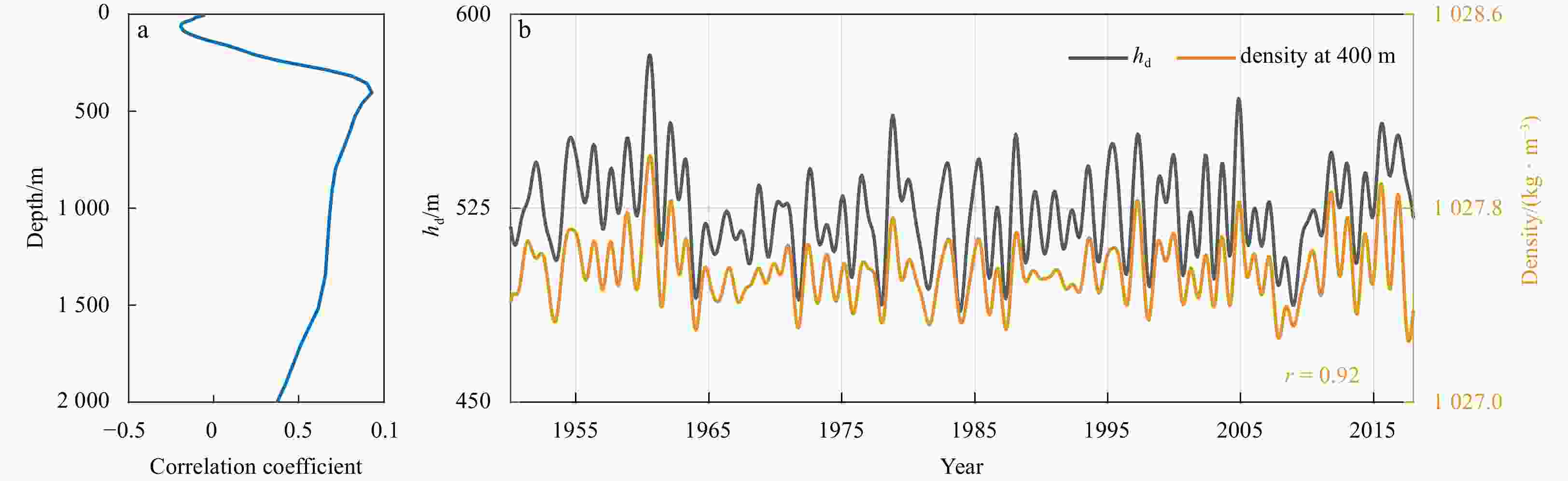
Figure  9.  Correlation coefficient between $ {h}_{\mathrm{d}} $ and the local density anomalies at different depths (a), and comparison of the interannual variability of $ {h}_{\mathrm{d}} $ (gray) and local density anomalies at 400 m (yellow) (b). The correlation coefficient is shown at the bottom in b.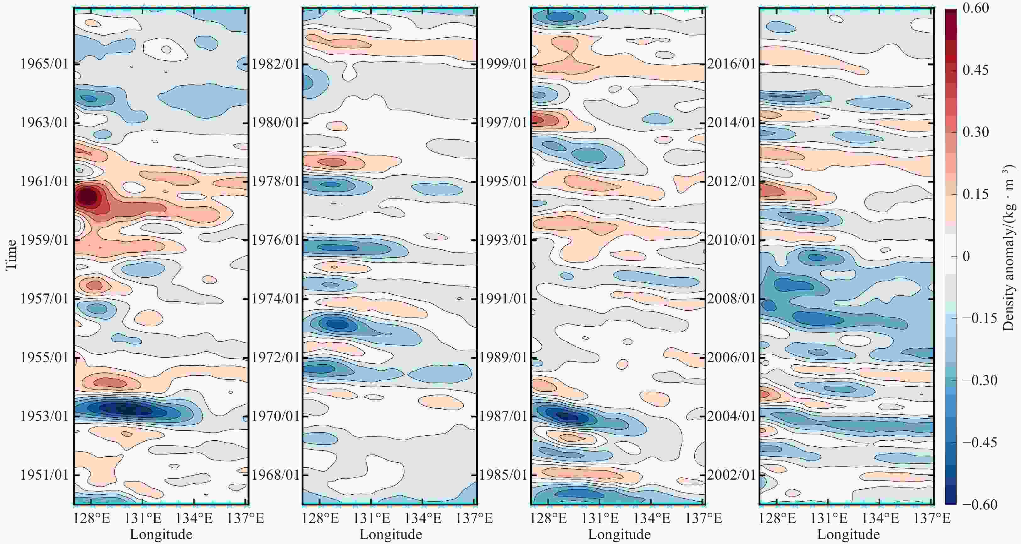

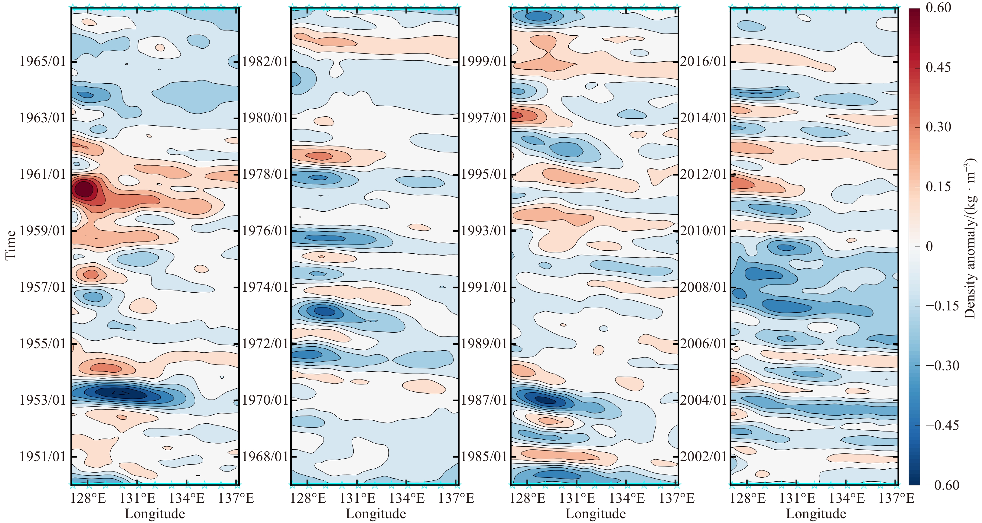
Figure  10.  Time-dependent density anomaly at 400 m during 1950–2017 along the path shown in Fig. 11a.

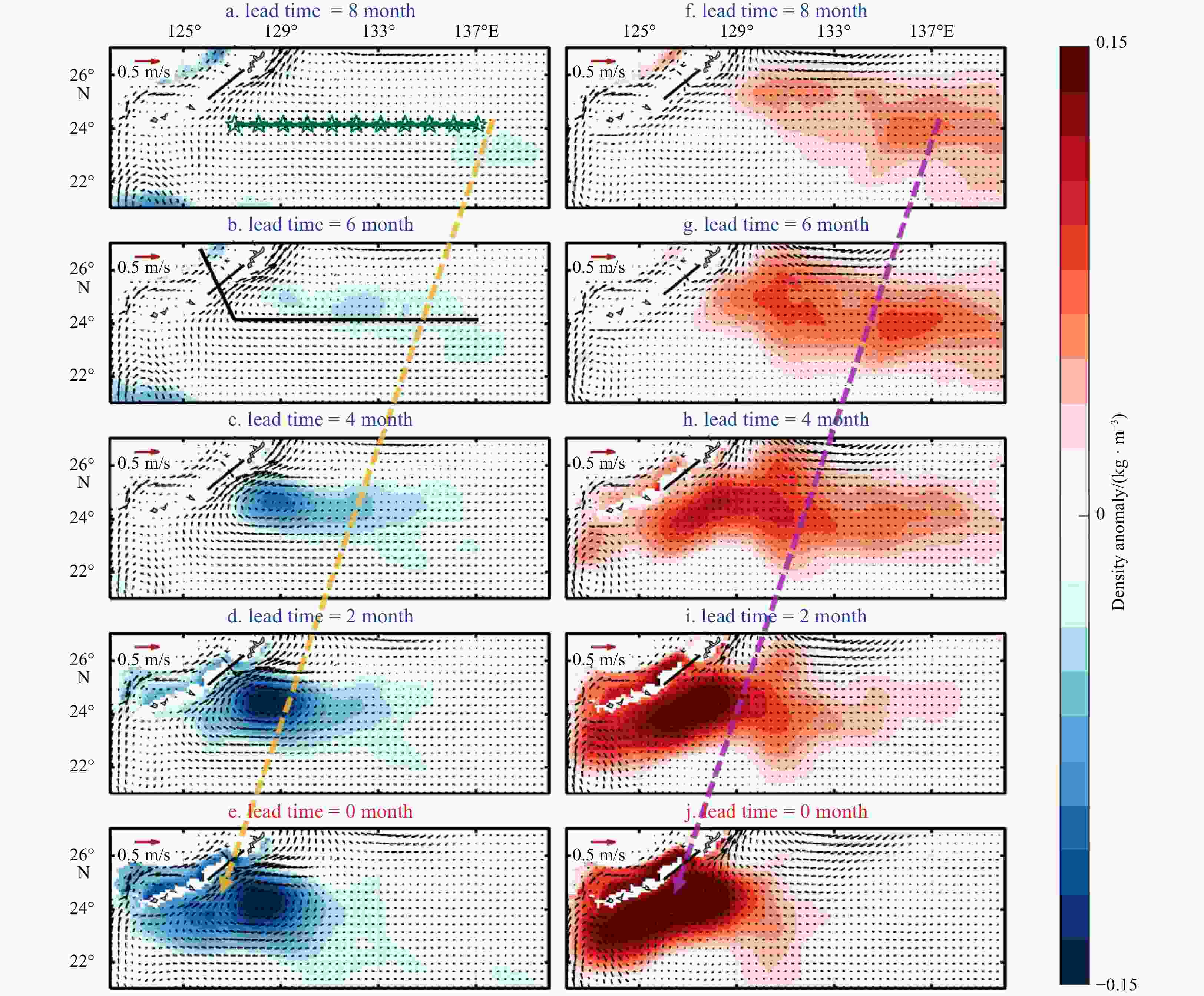
Figure  11.  Composite analysis of the density anomaly (shaded; unit: kg/m³) and horizontal velocity (vector; unit: m/s) at a depth of 400 m, with time leads 8 months (a), 6 months (b), 4 months (c), 2 months (d), and 0 month (e) for the positive KGT year, and the density anomaly and horizontal velocity at a depth of 400 m, with time leads 8 months (f), 6 months (g), 4 months (h), 2 months (i), and 0 month (j) for the negative KGT year. Only the negative density anomaly signals are shown in a–e and only the positive density anomaly signals are shown in f–j. The green line with stars in Fig. 11a represents the path followed to track the westward propagating density anomaly signals. The black line in Fig. 11b shows the section used to plot the vertical distribution of the density anomaly signals (Fig. 12). Ten yellow (purple) lines represent the propagation location of negative (positive) density anomaly signals.

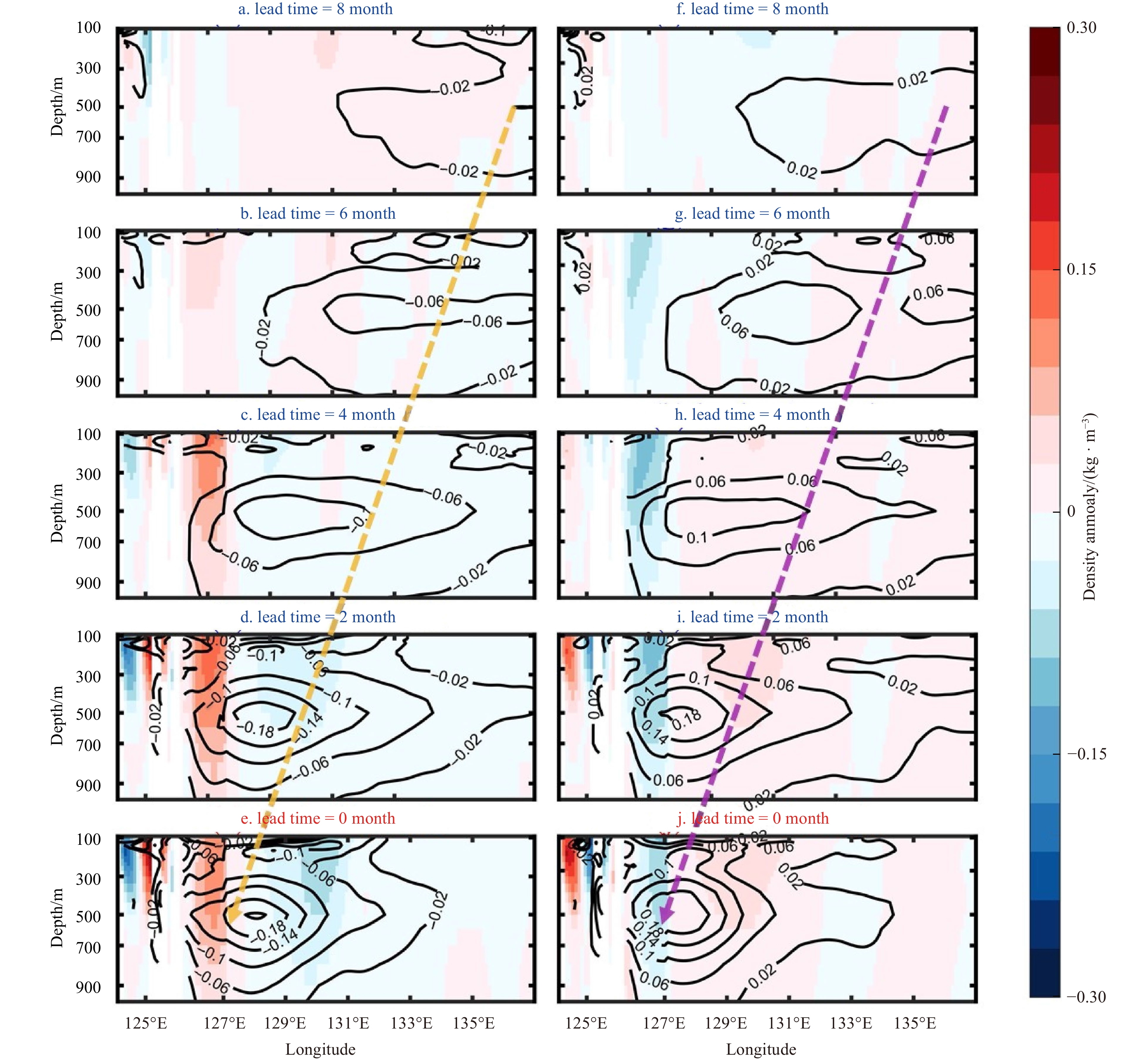
Figure  12.  Composite analysis of the vertical distribution of the density anomaly signals (contoured; unit: kg/m³) and the velocity anomalies (shaded; unit: m/s) perpendicular to the section shown in Fig. 11b, with time leads 8 months (a), 6 months (b), 4 months (c), 2 months (d), and 0 month (e) for the positive KGT year, 8 months (f), 6 months (g), 4 months (h), 2 months (i), and 0 month (j) for the negative KGT year. Ten yellow (purple) lines represent the propagation location of negative (postive) density anomaly signals.

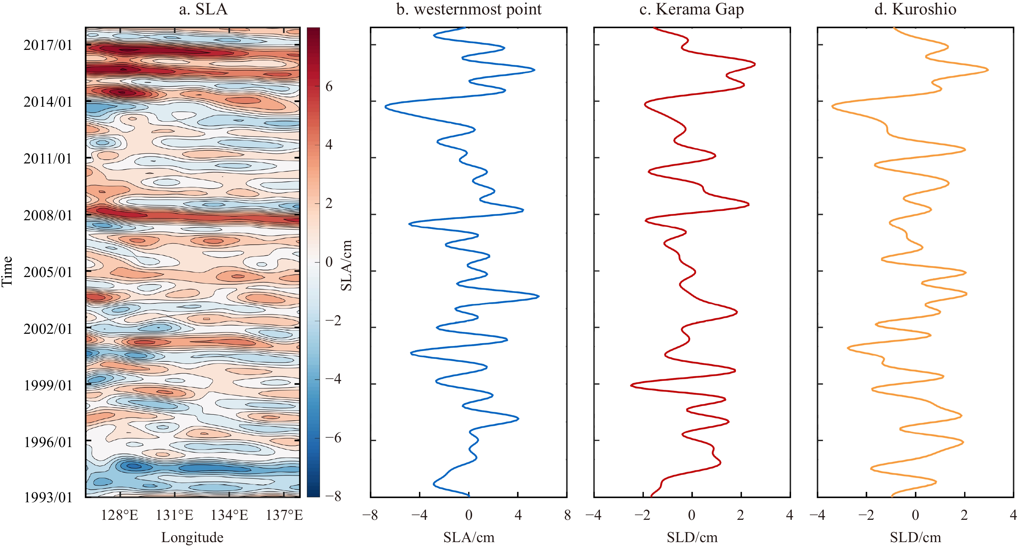
Figure  13.  Time-dependent SLA during 1993–2017 along the path shown in Fig. 11a (a), interannual variability of the SLA at the westernmost point of the path (b), interannual variability of the SLD between the two endpoints of the section of the Kerama Gap (south minus north) (c), and interannual variability of the SLD between the two endpoints of the Section 5 of the ECS-Kuroshio (east minus west) (d).

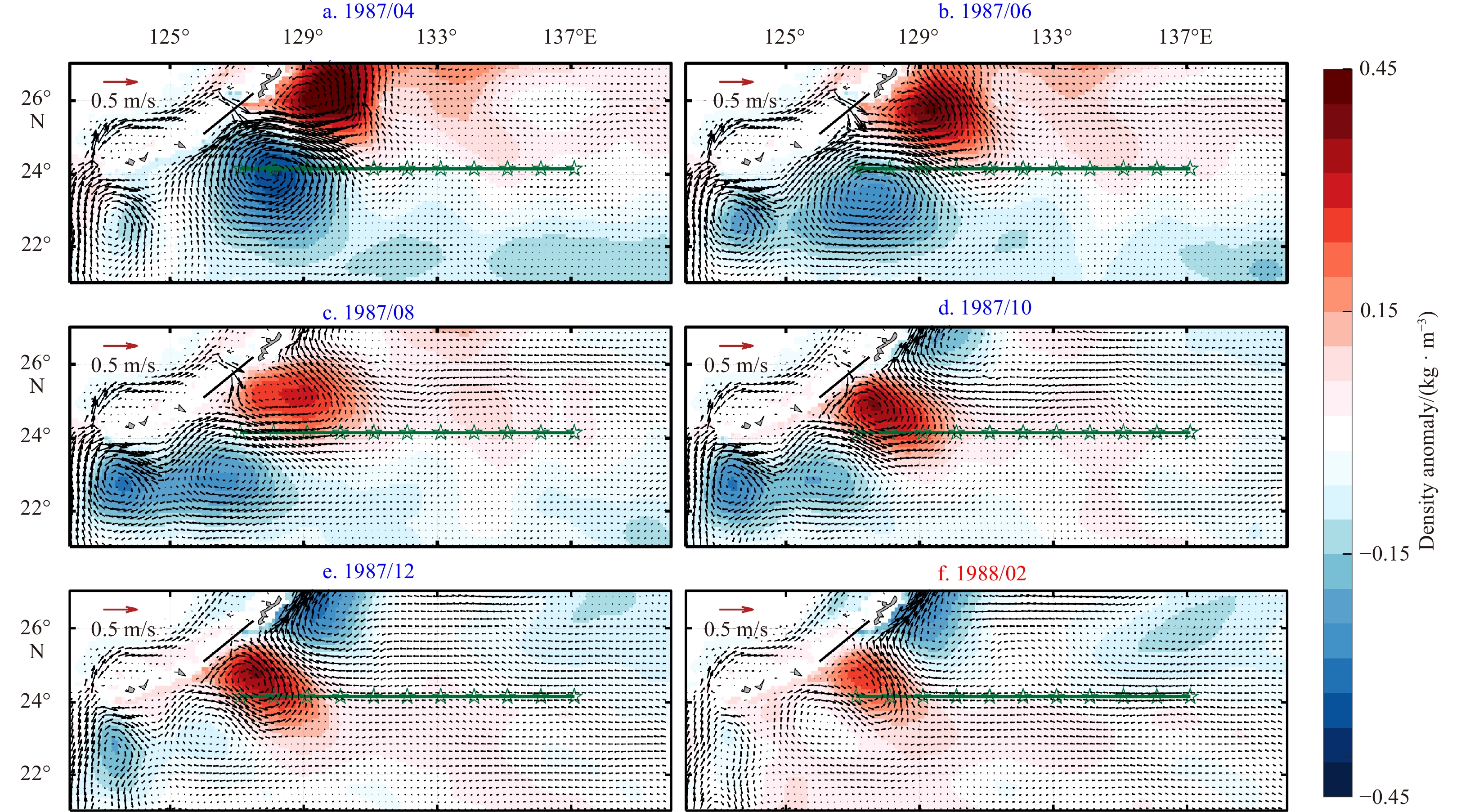
Figure  14.  A case analysis of the propagation of a positive density during April 1987 to February 1988. The vector represents the horizontal velocity and the shading represents the density anomaly at 500 m depth. The green line with stars represents the path followed to track the westward propagating density anomaly signals.