

Hyperspectral remote sensing identification of marine oil emulsions based on the fusion of spatial and spectral features
-
Abstract: Marine oil spill emulsions are difficult to recover, and the damage to the environment is not easy to eliminate. The use of remote sensing to accurately identify oil spill emulsions is highly important for the protection of marine environments. However, the spectrum of oil emulsions changes due to different water content. Hyperspectral remote sensing and deep learning can use spectral and spatial information to identify different types of oil emulsions. Nonetheless, hyperspectral data can also cause information redundancy, reducing classification accuracy and efficiency, and even overfitting in machine learning models. To address these problems, an oil emulsion deep-learning identification model with spatial-spectral feature fusion is established, and feature bands that can distinguish between crude oil, seawater, water-in-oil emulsion (WO), and oil-in-water emulsion (OW) are filtered based on a standard deviation threshold–mutual information method. Using oil spill airborne hyperspectral data, we conducted identification experiments on oil emulsions in different background waters and under different spatial and temporal conditions, analyzed the transferability of the model, and explored the effects of feature band selection and spectral resolution on the identification of oil emulsions. The results show the following. (1) The standard deviation–mutual information feature selection method is able to effectively extract feature bands that can distinguish between WO, OW, oil slick, and seawater. The number of bands was reduced from 224 to 134 after feature selection on the Airborne Visible Infrared Imaging Spectrometer (AVIRIS) data and from 126 to 100 on the S185 data. (2) With feature selection, the overall accuracy and Kappa of the identification results for the training area are 91.80% and 0.86, respectively, improved by 2.62% and 0.04, and the overall accuracy and Kappa of the identification results for the migration area are 86.53% and 0.80, respectively, improved by 3.45% and 0.05. (3) The oil emulsion identification model has a certain degree of transferability and can effectively identify oil spill emulsions for AVIRIS data at different times and locations, with an overall accuracy of more than 80%, Kappa coefficient of more than 0.7, and F1 score of 0.75 or more for each category. (4) As the spectral resolution decreasing, the model yields different degrees of misclassification for areas with a mixed distribution of oil slick and seawater or mixed distribution of WO and OW. Based on the above experimental results, we demonstrate that the oil emulsion identification model with spatial–spectral feature fusion achieves a high accuracy rate in identifying oil emulsion using airborne hyperspectral data, and can be applied to images under different spatial and temporal conditions. Furthermore, we also elucidate the impact of factors such as spectral resolution and background water bodies on the identification process. These findings provide new reference for future endeavors in automated marine oil spill detection.
-
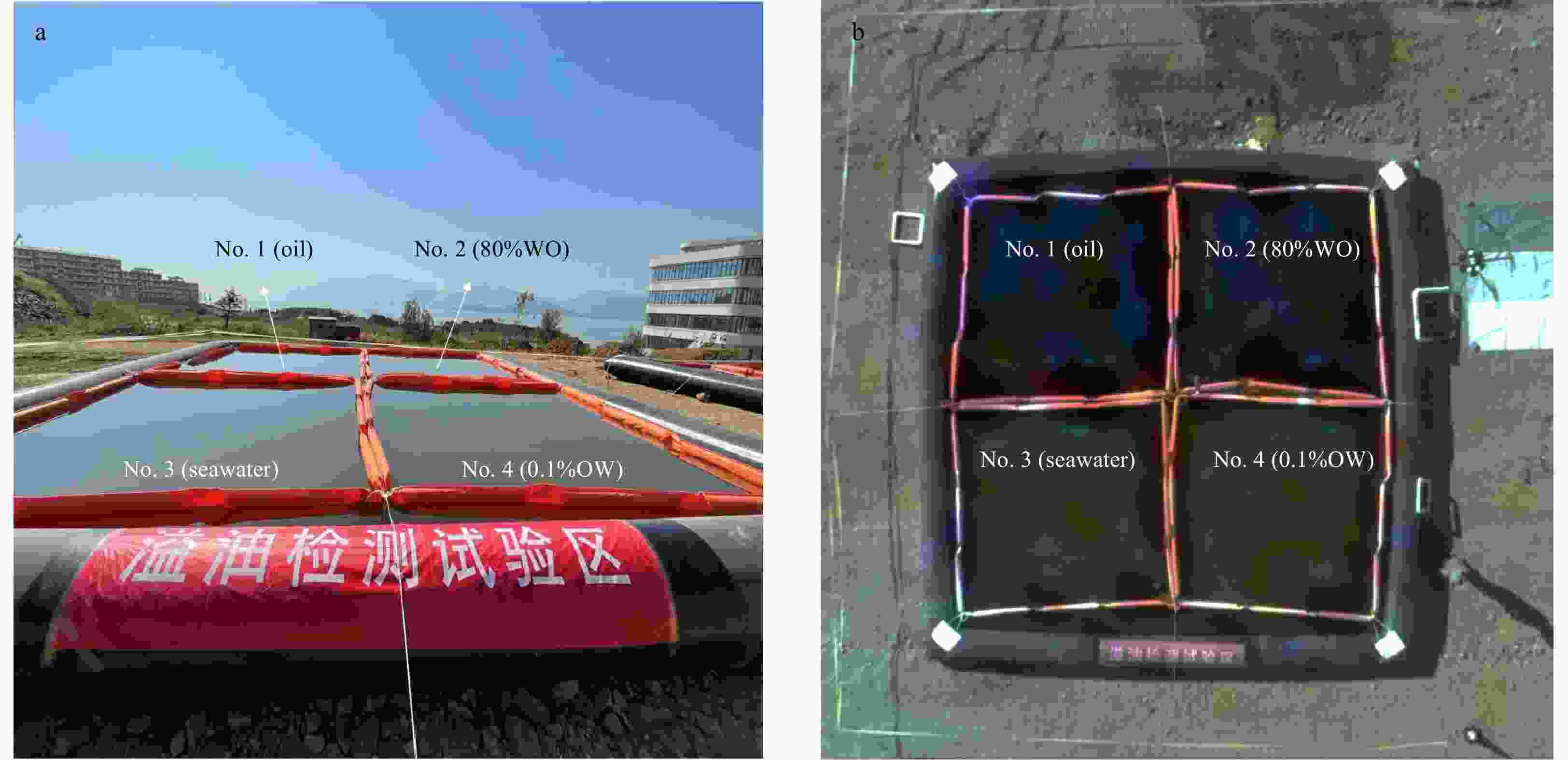
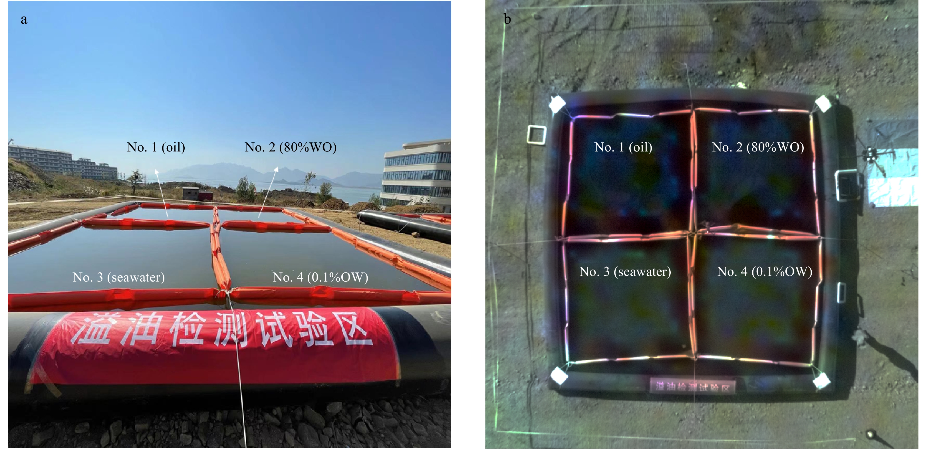
Figure 1. Setup of the experiments for the airborne hyperspectral observation of marine oil spills. a. Outfield oil spill hyperspectral observation experimental setup. b. Experimentally acquired S185 airborne hyperspectral image, true color composite: red: 638 nm, green: 550 nm, blue: 472 nm. The pool was divided into four enclosures injected with seawater. No. 1 was injected with crude oil, No. 2 was injected with WO at 80% volume concentration, No. 3 contained pure seawater and No. 4 was injected with OW at 0.1% volume concentration.
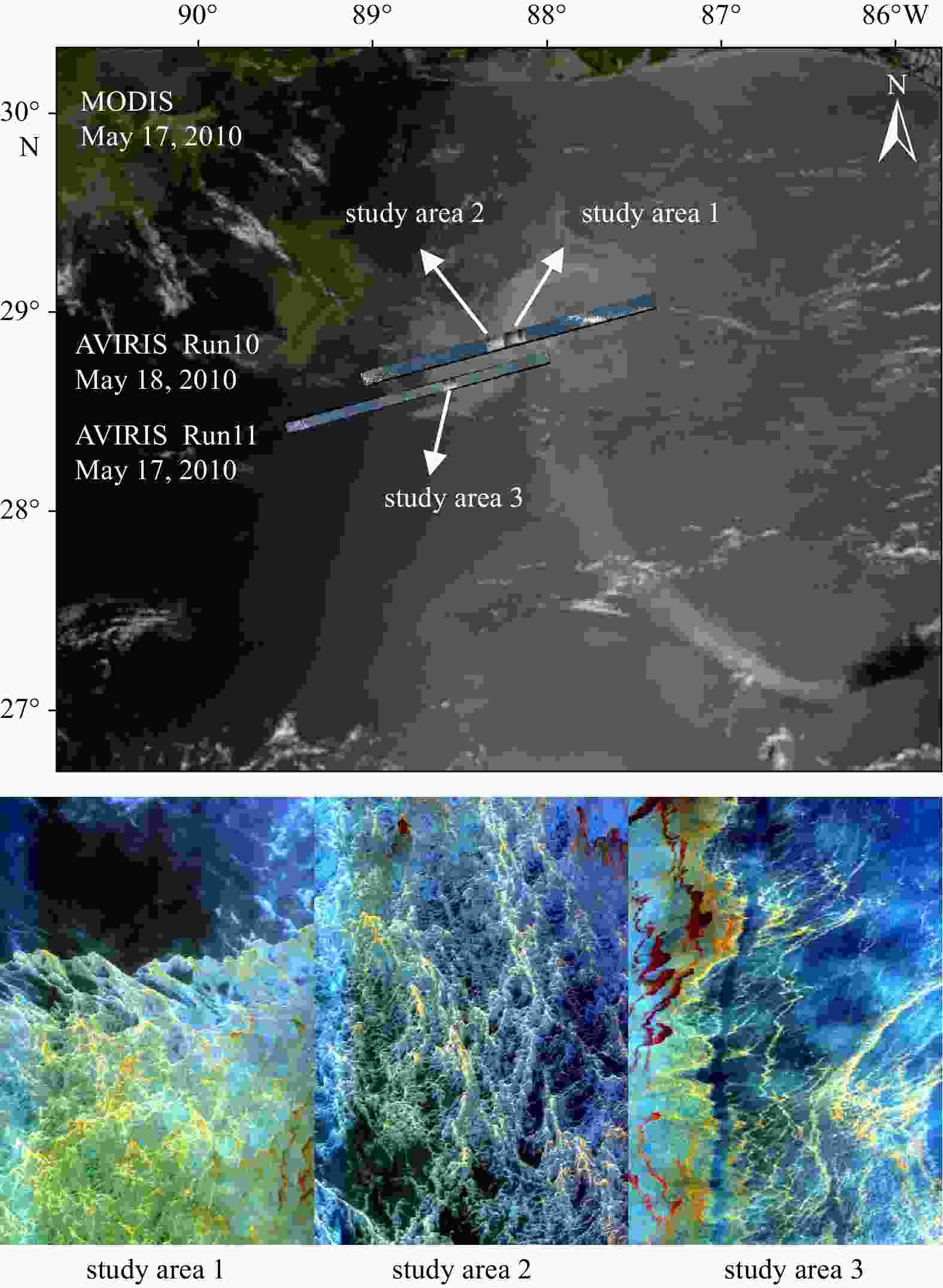
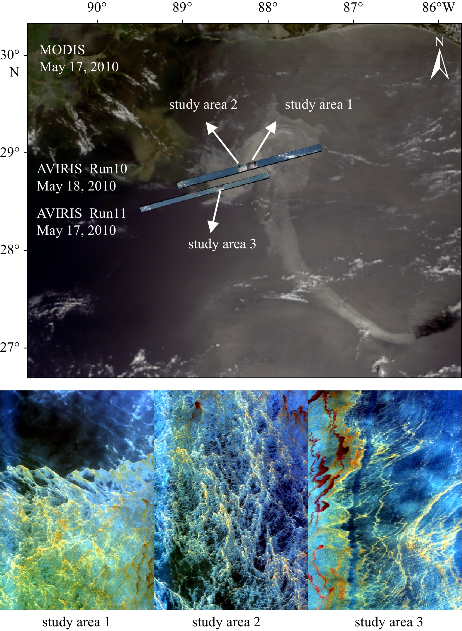
Figure 2. US Gulf of Mexico May 2010 AVIRIS true color composite image. For the subgraph located on the upper side, the study area overlaid on a MODIS image on 17 May 2010, true color composite. Study areas 1 and 2 were selected from the AVIRIS r10 image on 18 May 2010, and study area 3 was selected from an r11 image on 17 May 2010, true color composite: red: 638 nm, green: 550 nm, blue: 472 nm. Study area 1 is used for model training, study area 2 is used to evaluate the model’s spatial migration performance, and study area 3 is used to evaluate its spatial and temporal migration.
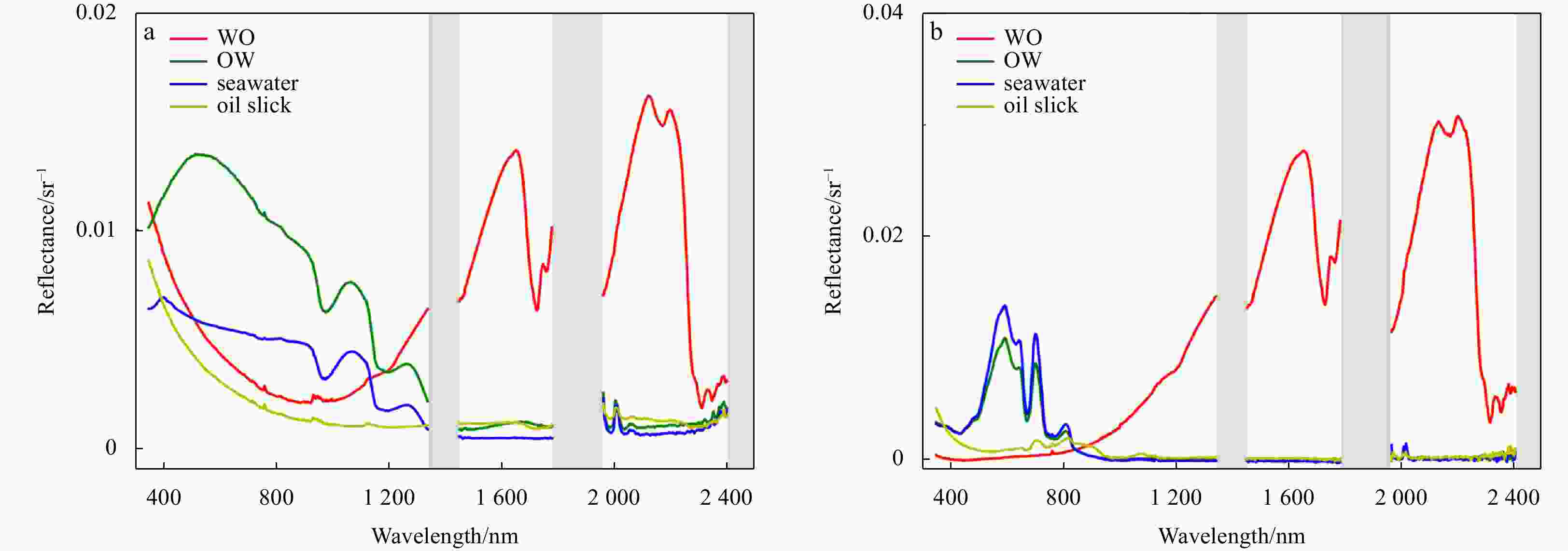
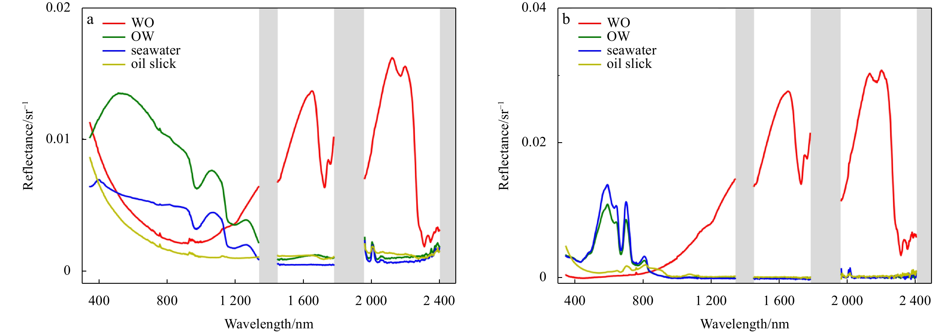
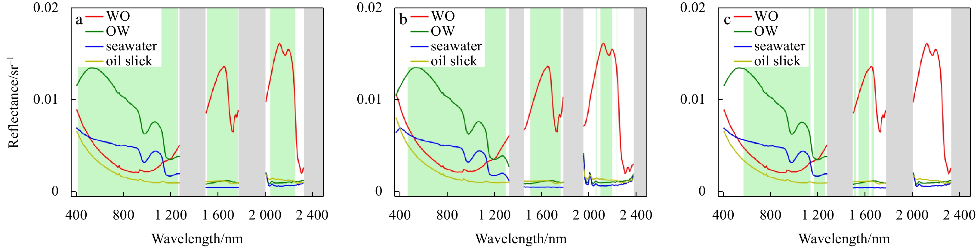
Figure 3. Outfield land-based experimental oil spill hyperspectral data. a. Hyperspectral data acquired in the context of a Class Ⅰ water body. b. Hyperspectral data acquired in the context of a Class Ⅱ water body. The grey bars indicate the atmospheric absorption bands.
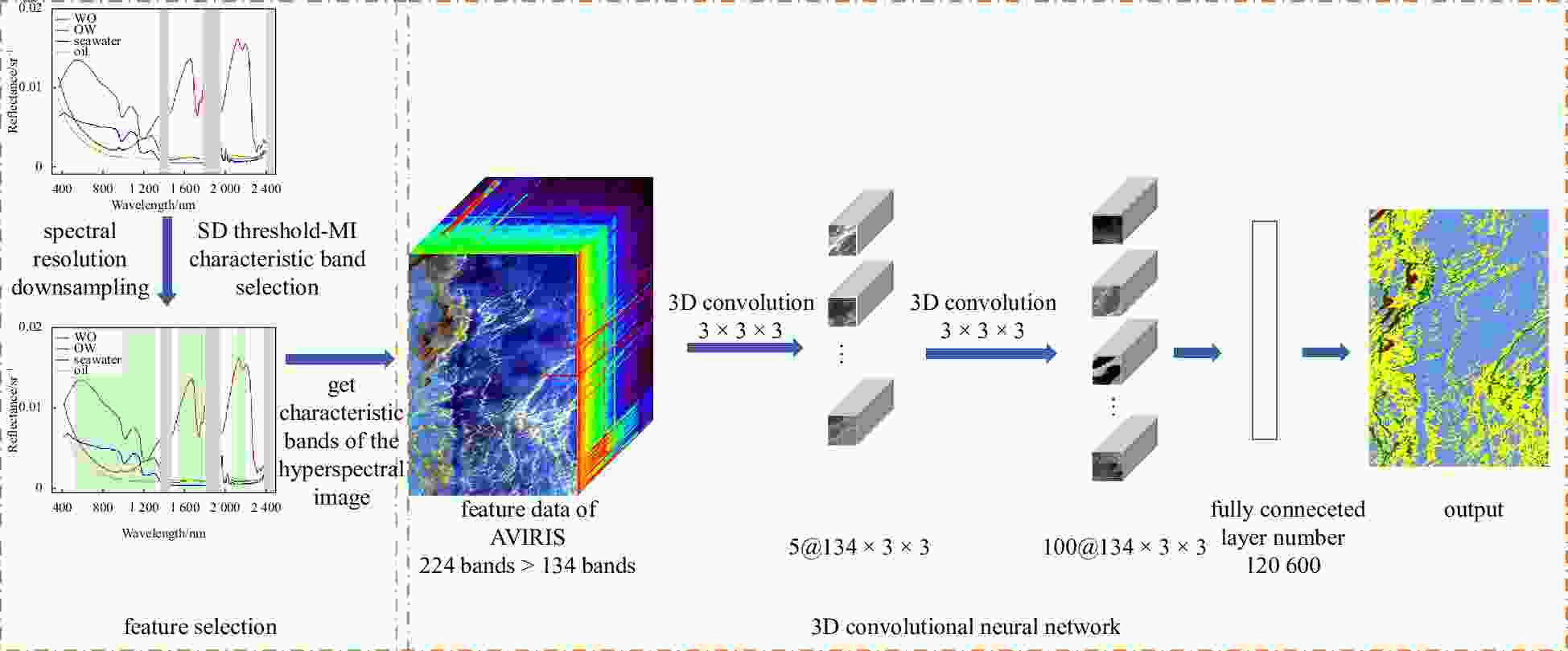
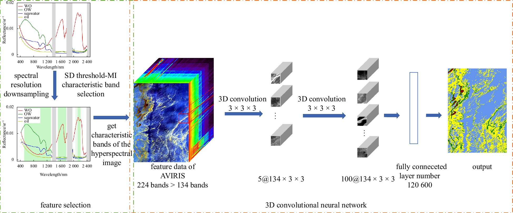
Figure 4. Oil emulsion identification model based on the fusion of spatial and spectral features.
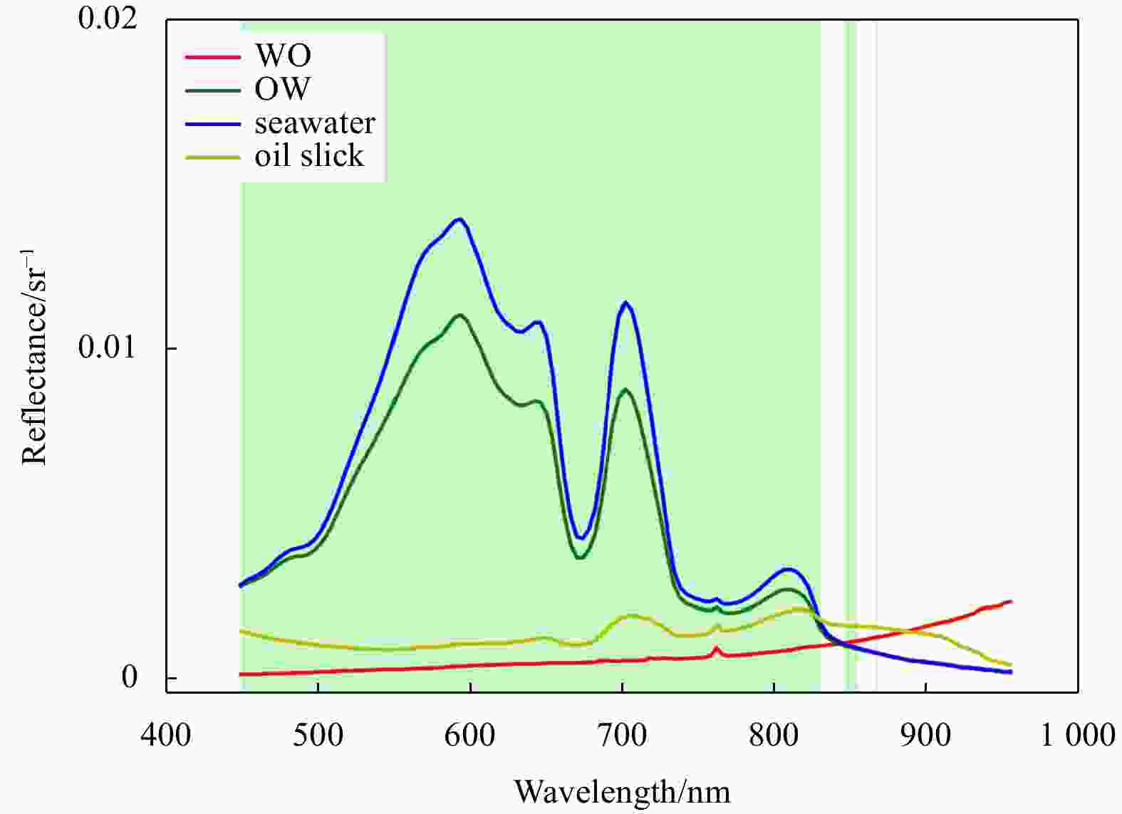
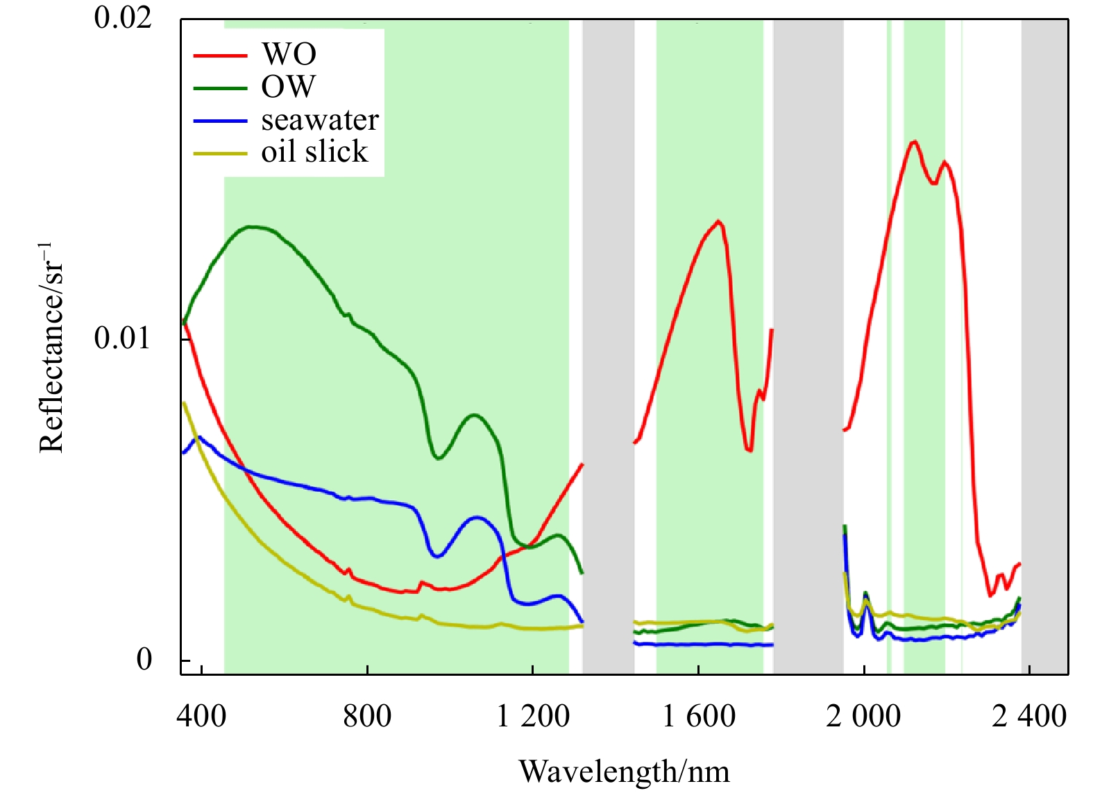
Figure 5. Hyperspectral data of oil spill emulsions in the context of a Class Ⅱ water body. The spectrum is downsampled to 126 bands, and the green bars are the selected feature band intervals.
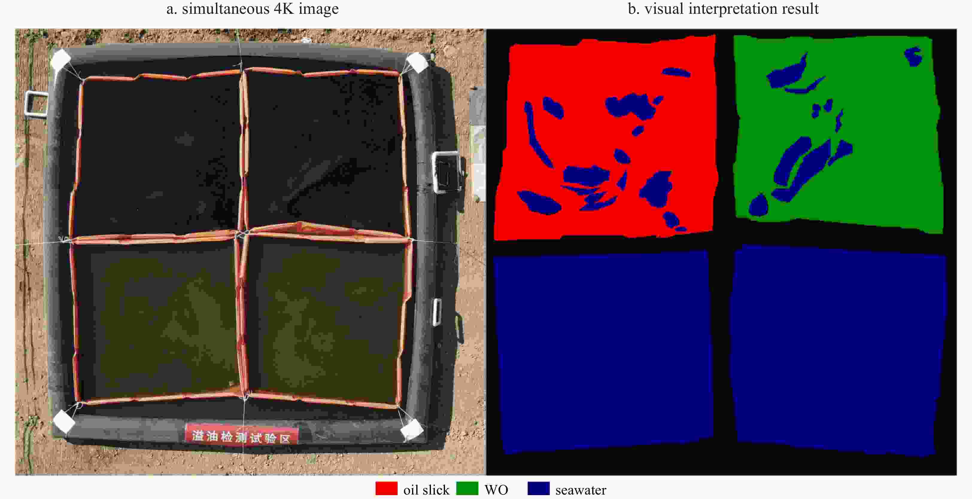
Figure 6. S185 airborne hyperspectral remote sensing imagery. a. Simultaneous 4K image; b. visual interpretation result. The upper left, upper right, lower left and lower right enclosures are numbered No. 1, No. 2, No. 3, and No. 4, respectively. No. 1 was filled with crude oil, No. 2 was filled with WO at a volume concentration of 80%, No. 3 contained pure seawater, and No. 4 contained OW at a volume concentration of 0.1%.

Figure 7. Results of airborne hyperspectral image identification for outfield experiments. a. Identification result. b. 4K image.
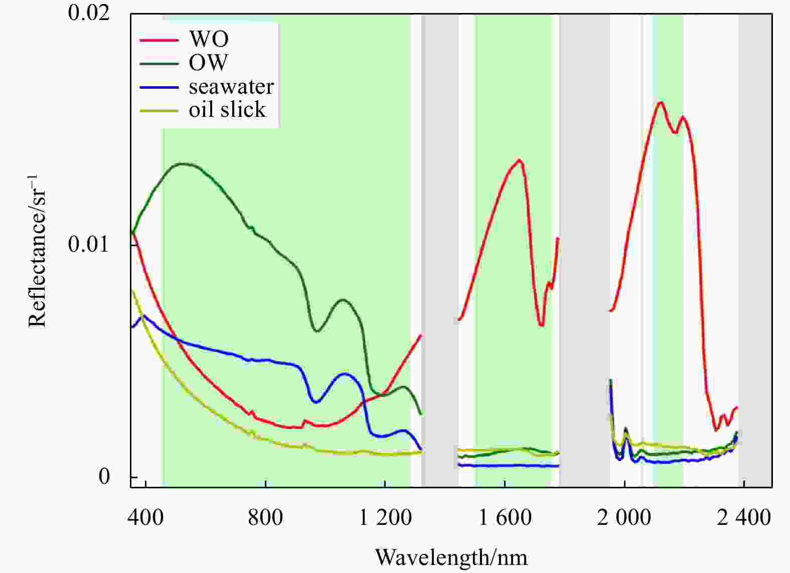
Figure 8. Hyperspectral data of oil emulsions in the context of a Class Ⅰ water body. The spectrum is downsampled to 224 bands. The green bars are the selected feature band intervals and the grey bars are the atmospheric absorption bands.
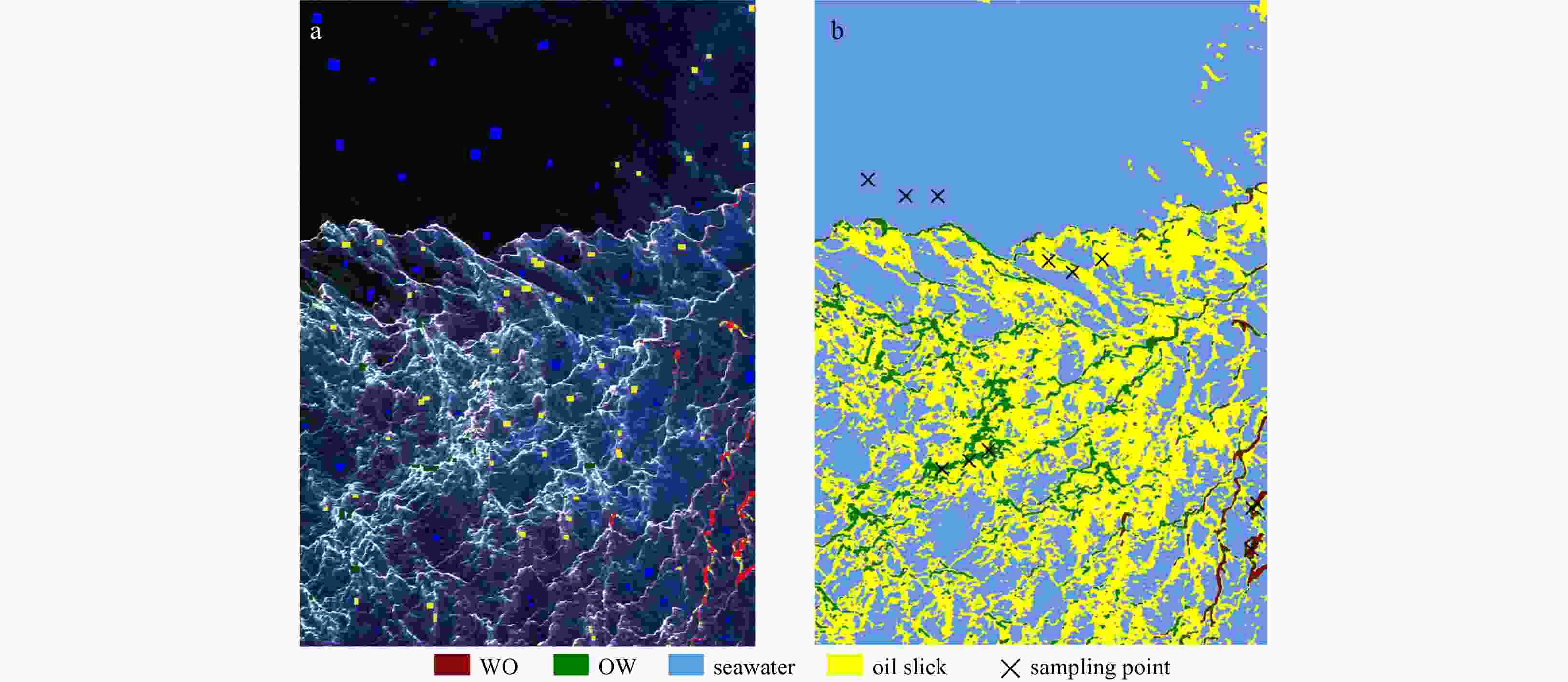
Figure 9. Study area 1 label distribution and identification results. a. Label distribution. The image is a false color composite: red: 1672 nm, green: 832 nm, blue: 658 nm. b. Identification results.
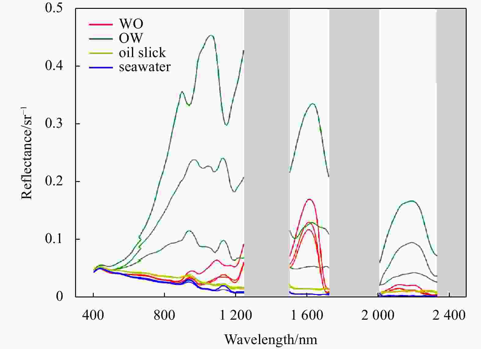
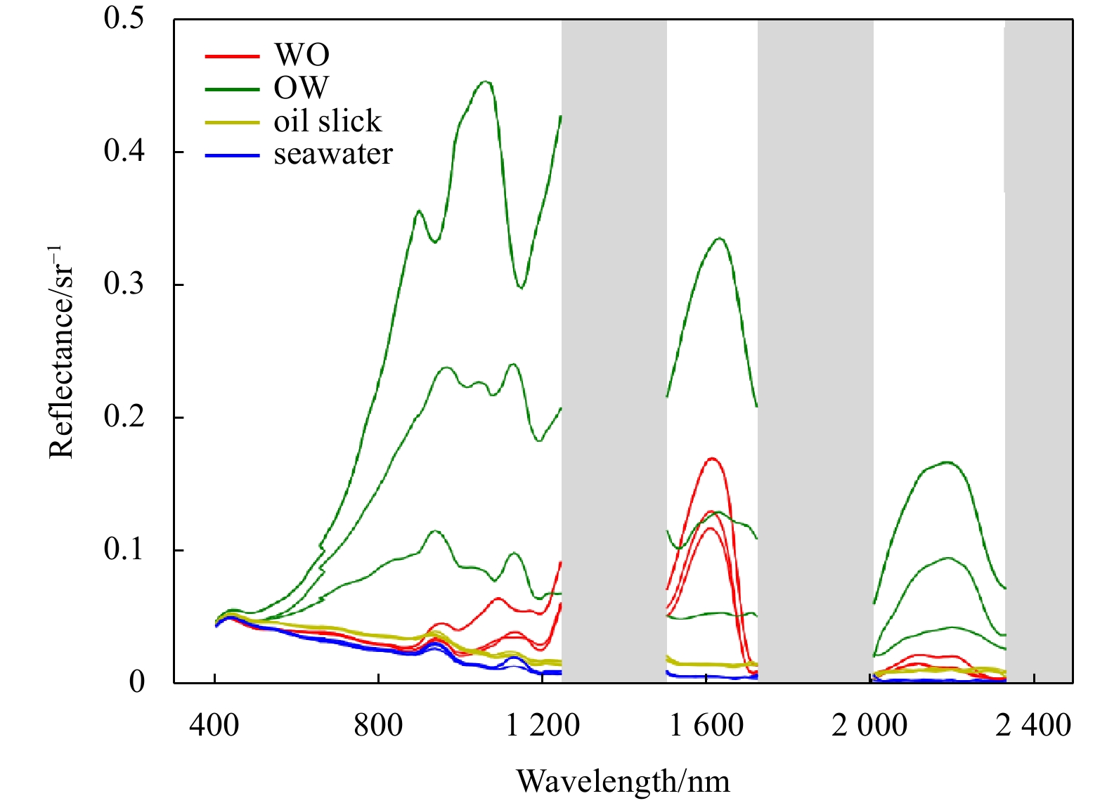
Figure 10. Spectral reflectance of sampled pixels in study area 1. The grey bars are the atmospheric absorption bands.
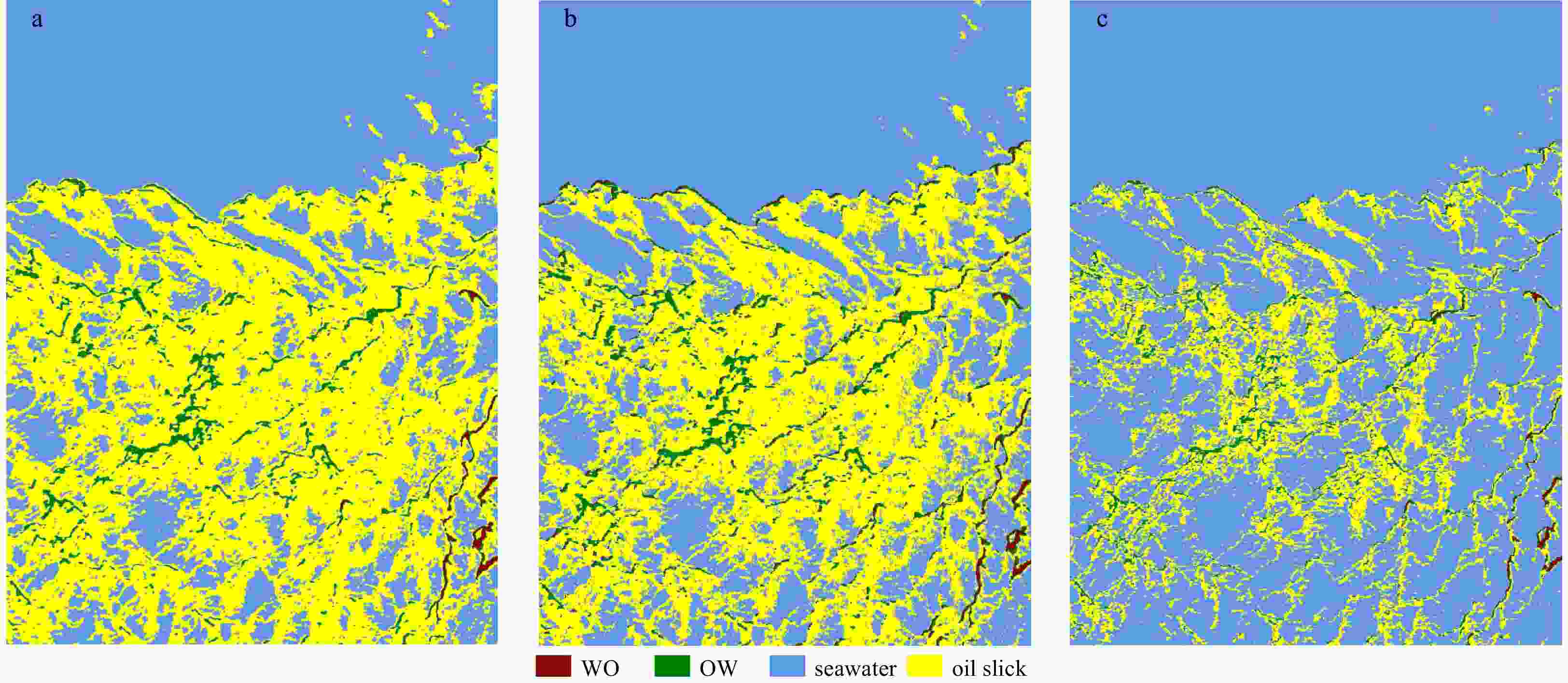
Figure 11. Identification results of different classifiers for study area 1. a. 2D-CNN classifier identification results. b. 1D-CNN classifier identification results. c. SVM classifier identification results.
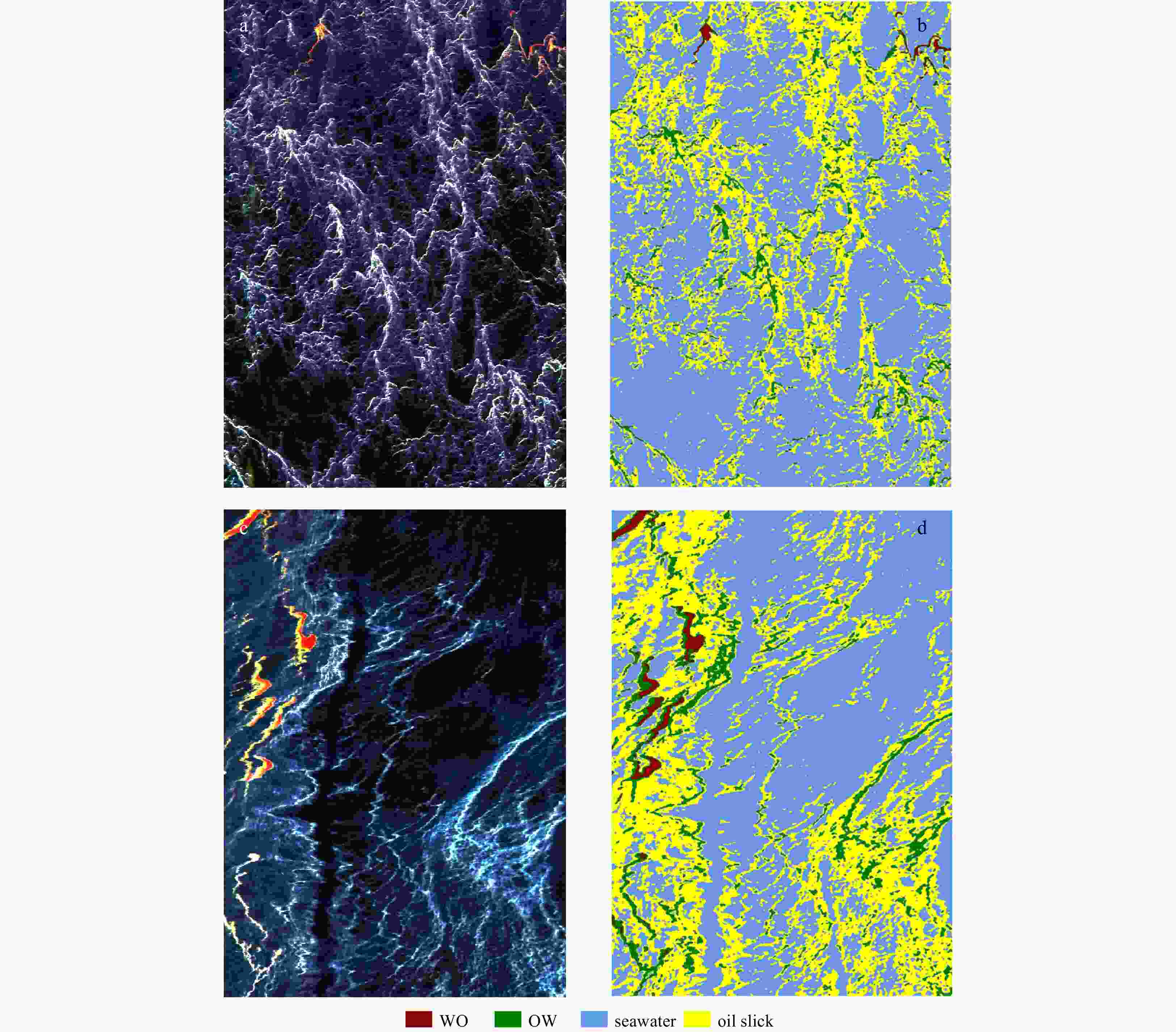
Figure 12. Spatial and temporal migration identification results obtained by the oil emulsion identification model. a and c. Study areas 2 and 3, respectively, false-color composite: red: 1672 nm, green: 832 nm, blue: 658 nm. b and d. The model identification results of a and c, respectively. Study area 2 is a spatial migration area of study area 1 and study area 3 is a spatial–temporal migration area of study area 1.
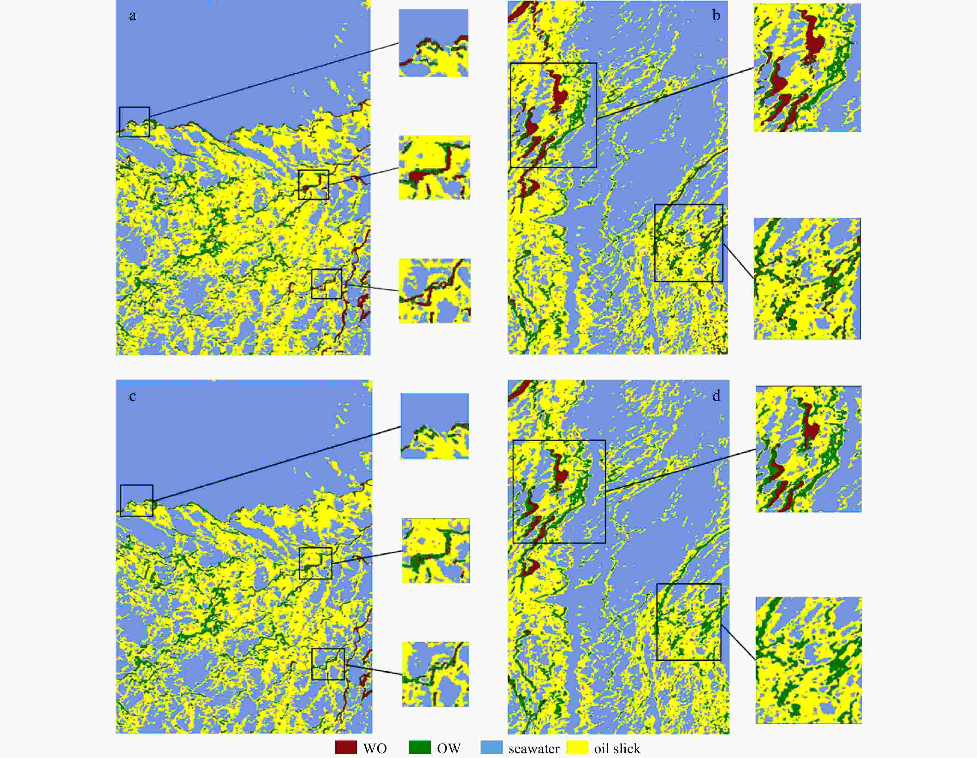
Figure 13. Comparison of the identification results with and without feature selection in study areas 1 and 3. a and b. Identification results obtained without feature selection for study areas 1 and 3, respectively. c and d. Identification results obtained with feature selection for study areas 1 and 3, respectively.
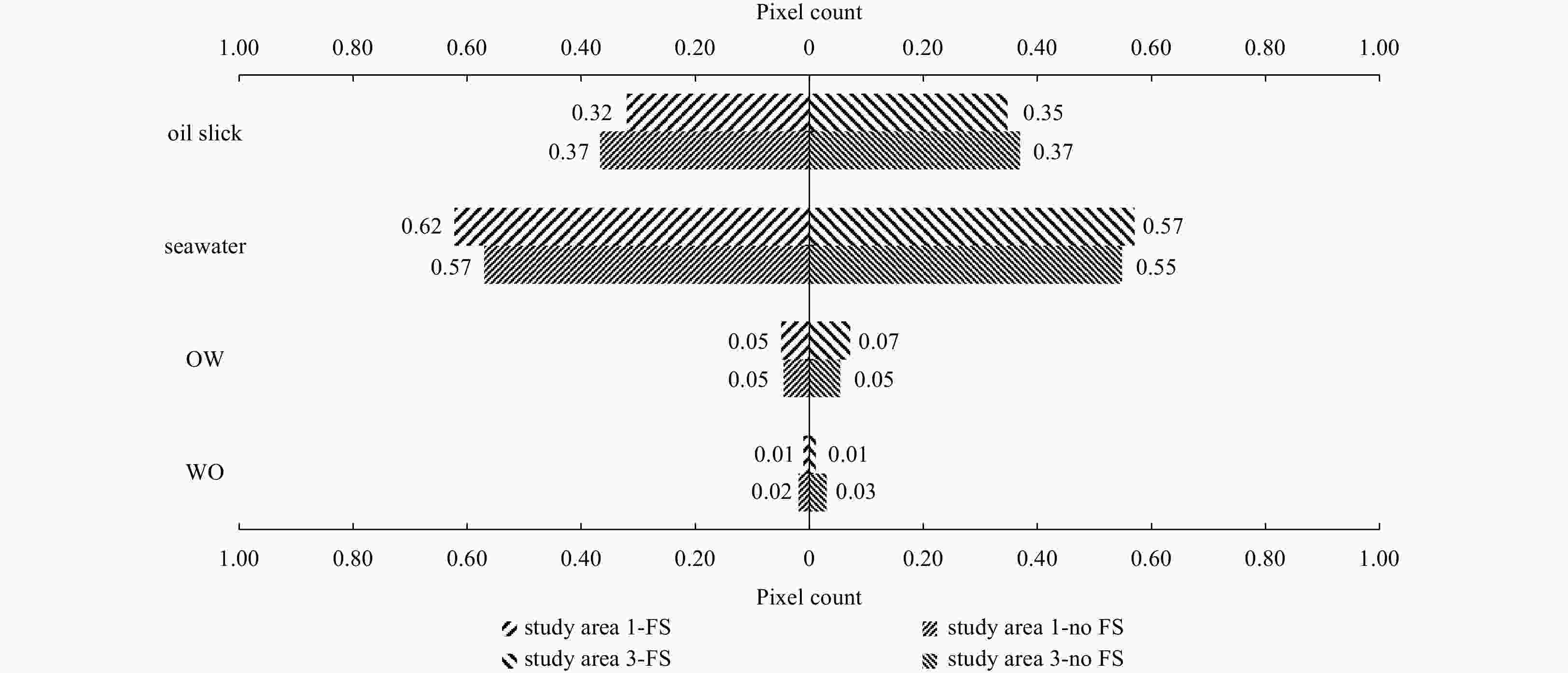
Figure 14. Pixels statistics of the identification results obtained with feature selection (FS) and without feature selection (no FS) in study areas 1 and 3.
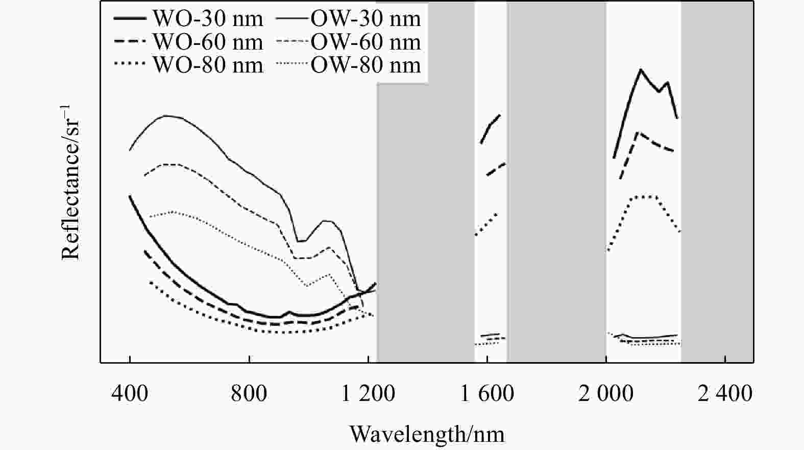
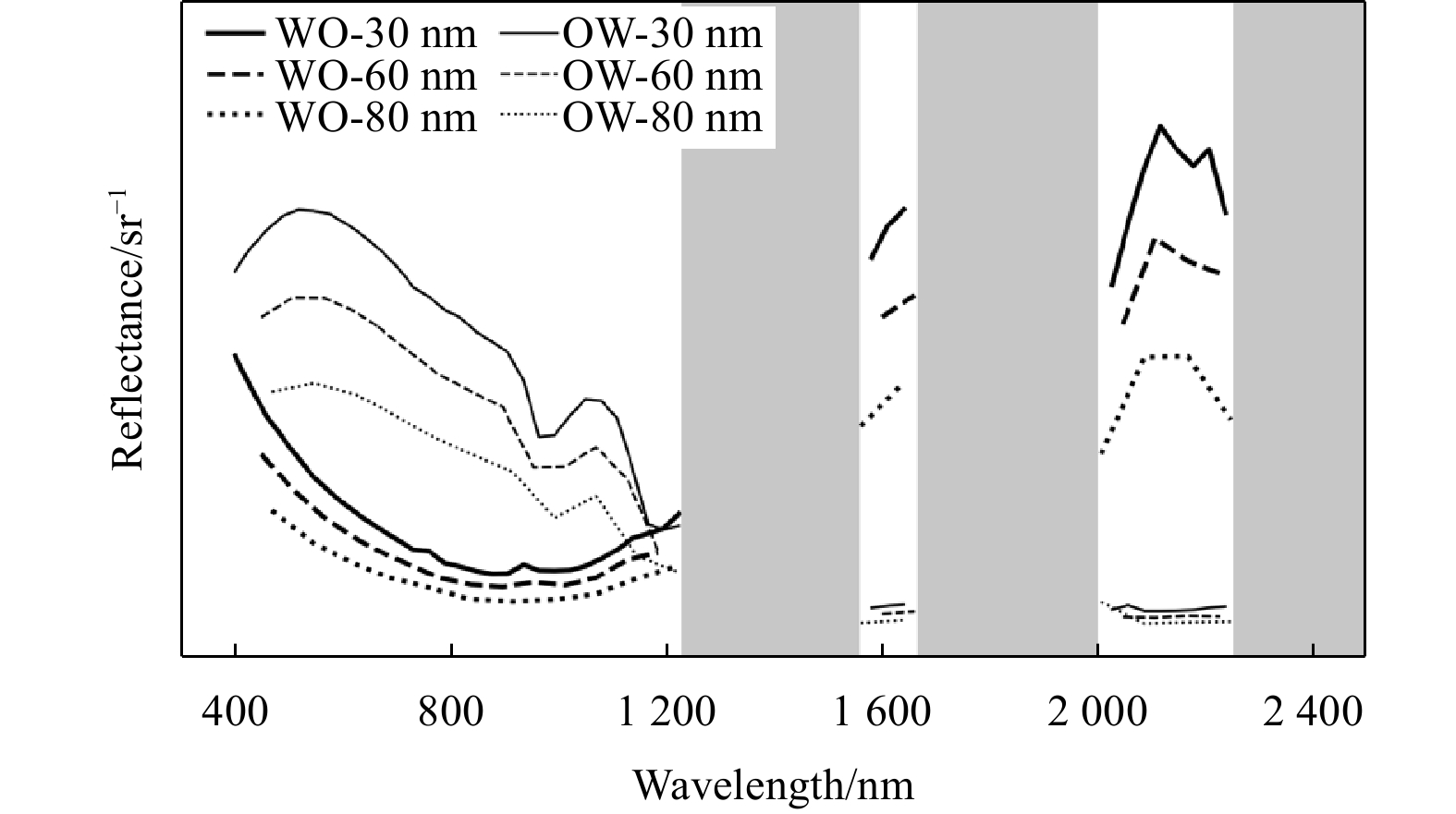
Figure 15. AVIRIS spectrally downsampled data obtained from the ASD data. For the convenience of plotting, the reflectance data has been scaled as a whole and the y-axis does not display the reflectance values.

Figure 16. Identification results at different spectral resolutions for study areas 1 and 3. a, b and c. Results of the identification of study area 1 at spectral resolutions of 30 nm, 60 nm and 80 nm, respectively. d, e and f. Results of the identification of study area 3 at spectral resolutions of 30 nm, 60 nm and 80 nm, respectively.
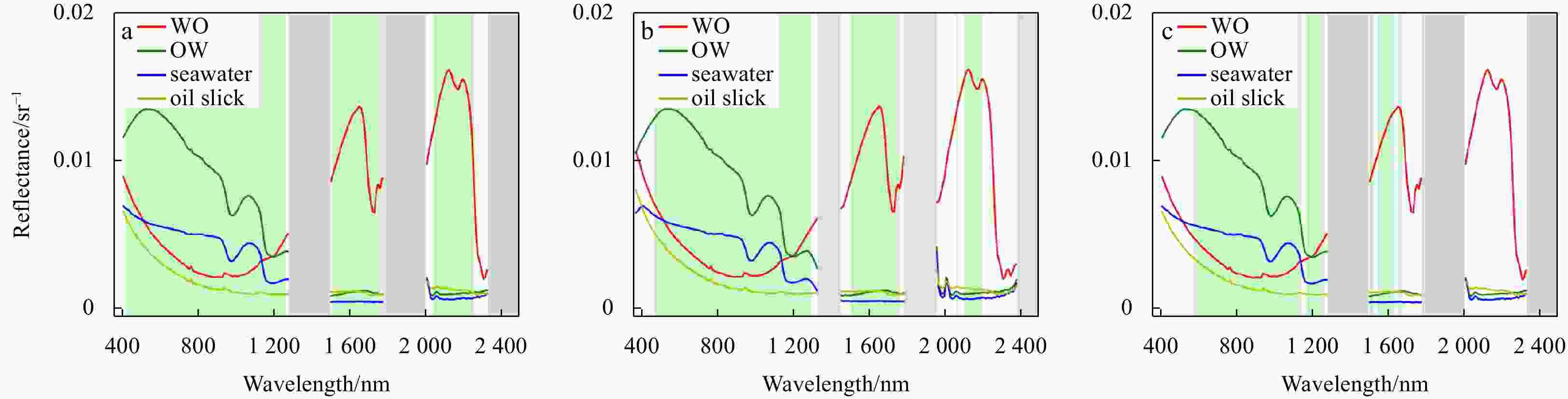
Figure 17. Feature selection results for different MI thresholds. a, b and c. Results of feature band selection for MI thresholds of 0.6, 0.7 and 0.8, respectively. The green bars are the selected feature band intervals and the grey bars are the atmospheric absorption bands.

Figure 18. Model identification results for different convolutional kernel sizes. a, b and c. Identification results for study areas 1, 2 and 3, respectively, when the convolution kernel is 5 × 3 × 3. d, e and f. Identification results for study areas 1, 2 and 3, respectively, when the convolution kernel is 7 × 3 × 3.
Table 1. Accuracy evaluation of the airborne hyperspectral image identification results for the outfield experiments
Target Precision Recall F1 score WO 0.92 0.96 0.94 Seawater 0.93 0.94 0.93 Oil slick 0.97 0.95 0.96  下载: 导出CSV
Table 2. Accuracy evaluation of identification results for study area 1
Target Precision Recall F1 score WO 0.78 0.94 0.85 OW 0.83 0.82 0.82 Seawater 0.96 0.98 0.97 Oil slick 0.93 0.78 0.85
下载: 导出CSV
Table 3. Comparison of the overall accuracy (OA) of the identification results using different classifiers in study area 1
Classifier (OA and
Kappa coefficient)Target Precision Recall F1 score 2D-CNN (OA = 87.02%,
Kappa coefficient = 0.78)WO 0.62 0.98 0.76 OW 0.87 0.72 0.79 seawater 0.90 0.99 0.94 oil slick 0.97 0.64 0.77 1D-CNN (OA = 87.82%,
Kappa coefficient = 0.82)WO 0.46 0.98 0.63 OW 0.91 0.78 0.84 seawater 0.99 0.93 0.96 oil slick 0.92 0.85 0.88 SVM (OA = 87.93%,
Kappa coefficient = 0.78)WO 0.72 0.99 0.83 OW 0.87 0.92 0.89 seawater 0.99 0.87 0.93 oil slick 0.61 0.84 0.71
下载: 导出CSV
Table 4. Accuracy evaluation of the identification results for study area 2
Target Precision Recall F1 score WO 0.85 0.73 0.79 OW 0.8 0.99 0.88 Seawater 0.99 0.7 0.82 Oil slick 0.63 0.93 0.75
下载: 导出CSV
Table 5. Accuracy evaluation of the identification results for study area 3
Target Precision Recall F1 score WO 0.98 0.79 0.87 OW 0.72 0.98 0.83 Seawater 0.95 0.83 0.97 Oil slick 0.78 0.93 0.85
下载: 导出CSV
Table 6. Accuracy evaluation of the identification results for study area 1
Target No FS or FS Precision Recall F1 score WO no FS 0.83 0.86 0.84 FS 0.78 0.94 0.85 OW no FS 0.55 0.82 0.66 FS 0.83 0.82 0.82 Seawater no FS 0.93 0.97 0.95 FS 0.96 0.98 0.97 Oil slick no FS 0.92 0.74 0.82 FS 0.93 0.78 0.85 Note: Each type of target corresponds to two columns of accuracy evaluation results. The first column is the accuracy of the identification results without feature selection (no FS), and the second column is the accuracy of identification results with feature selection (FS).
下载: 导出CSV
Table 7. Accuracy evaluation of identification results for study area 3
Target No FS or FS Precision Recall F1 score WO no FS 0.99 0.61 0.75 FS 0.98 0.79 0.87 OW no FS 0.35 1.00 0.52 FS 0.72 0.98 0.83 Seawater no FS 0.95 0.85 0.90 FS 0.95 0.83 0.97 Oil slick no FS 0.82 0.93 0.87 FS 0.78 0.93 0.85 Note: Each type of target corresponds to two columns of accuracy evaluation results. The first column is the accuracy of identification results without feature selection (no FS), and the second column is the accuracy of identification results with feature selection (FS).
下载: 导出CSV
Table 8. Comparison of the overall accuracy (OA) of the identification results at different spectral resolutions (SR) in study area 1
SR (OA and Kappa
coefficient)Target Precision Recall F1 score SR = 30 nm (OA = 90.46%,
Kappa coefficient = 0.84)WO 0.86 0.85 0.85 OW 0.49 0.81 0.61 seawater 0.94 0.98 0.96 oil slick 0.94 0.93 0.93 SR = 60 nm (OA = 90.40%,
Kappa coefficient = 0.83)WO 0.8 0.85 0.82 OW 0.51 0.79 0.62 seawater 0.98 0.96 0.97 oil slick 0.86 0.8 0.83 SR = 80 nm (OA = 89.41%,
Kappa coefficient = 0.82)WO 0.77 0.85 0.81 OW 0.54 0.87 0.67 seawater 0.94 0.99 0.96 oil slick 0.95 0.71 0.81
下载: 导出CSV
Table 9. Comparison of the overall accuracy (OA) of the identification results at different spectral resolutions (SRs) in study area 3
SR (OA and Kappa
coefficient)Target Precision Recall F1 score SR = 30 nm, OA = 80.80%,
Kappa = 0.72WO 1.00 0.56 0.72 OW 0.23 1.00 0.37 seawater 0.95 0.84 0.89 oil slick 0.79 0.93 0.85 SR = 60 nm, OA = 83.23%,
Kappa = 0.76WO 1.00 0.73 0.84 OW 0.63 1.00 0.77 seawater 0.97 0.78 0.86 oil slick 0.69 0.95 0.80 SR = 80 nm, OA = 80.53%,
Kappa = 0.72WO 1.00 0.57 0.73 OW 0.24 1.00 0.39 seawater 0.90 0.87 0.88 oil slick 0.84 0.88 0.86
下载: 导出CSV
-
Du Kai, Ma Yi, Jiang Zongchen, et al. 2022. Detection of oil spill based on CBF-CNN using HY-1C CZI multispectral images. Acta Oceanologica Sinica, 41(7): 166–179, doi: 10.1007/s13131-021-1977-x Fauvel M, Tarabalka Y, Benediktsson J A, et al. 2013. Advances in spectral-spatial classification of hyperspectral images. Proceedings of the IEEE, 101(3): 652–675, doi: 10.1109/JPROC.2012.2197589 Hu Chuanmin, Lu Yingcheng, Sun Shaojie, et al. 2021. Optical remote sensing of oil spills in the ocean: what is really possible?. Journal of Remote Sensing, 2021: 9141902 Jiang Zongchen, Ma Yi. 2020. Accurate extraction of offshore raft aquaculture areas based on a 3D-CNN model. International Journal of Remote Sensing, 41(14): 5457–5481, doi: 10.1080/01431161.2020.1737340 Jiao Junnan, Lu Yingcheng, Liu Yongxue. 2022. Optical quantification of oil emulsions in multi-band coarse-resolution imagery using a lab-derived HSV model. Marine Pollution Bulletin, 178: 113640, doi: 10.1016/j.marpolbul.2022.113640 Leifer I, Lehr W J, Simecek-Beatty D, et al. 2012. State of the art satellite and airborne marine oil spill remote sensing: application to the BP Deepwater Horizon oil spill. Remote Sensing of Environment, 124: 185–209, doi: 10.1016/j.rse.2012.03.024 Li Ying, Yu Qinglai, Xie Ming, et al. 2021. Identifying oil spill types based on remotely sensed reflectance spectra and multiple machine learning algorithms. IEEE Journal of Selected Topics in Applied Earth Observations and Remote Sensing, 14: 9071–9078, doi: 10.1109/JSTARS.2021.3109951 Lu Yingcheng, Hu Chuanmin, Sun Shaojie, et al. 2016. Overview of optical remote sensing of marine oil spills and hydrocarbon seepage. Journal of Remote Sensing (in Chinese), 20(5): 1259–1269 Lu Yingcheng, Shi Jing, Hu Chuanmin, et al. 2020. Optical interpretation of oil emulsions in the ocean—Part II: Applications to multi-band coarse-resolution imagery. Remote Sensing of Environment, 242: 111778, doi: 10.1016/j.rse.2020.111778 Lu Yingcheng, Shi Jing, Wen Yansha, et al. 2019. Optical interpretation of oil emulsions in the ocean—Part I: Laboratory measurements and proof-of-concept with AVIRIS observations. Remote Sensing of Environment, 230: 111183, doi: 10.1016/j.rse.2019.05.002 Lu Yingcheng, Tian Qingjiu, Wang Jingjing, et al. 2008. Experimental study of the spectral response of oil films on the sea surface. Chinese Science Bulletin (in Chinese), 53(9): 1085–1088, doi: 10.1360/csb2008-53-9-1085 Qin Fangjin, Zhang Aiwu, Wang Shumin, et al. 2015. Hyperspectral band selection based on spectral clustering and inter-class separability factor. Spectroscopy and Spectral Analysis (in Chinese), 35(5): 1357–1364 Ross B C. 2014. Mutual information between discrete and continuous data sets. PLoS One, 9(2): e87357, doi: 10.1371/journal.pone.0087357 Shi Jing, Jiao Junnan, Lu Yingcheng, et al. 2018. Determining spectral groups to distinguish oil emulsions from Sargassum over the Gulf of Mexico using an airborne imaging spectrometer. ISPRS Journal of Photogrammetry and Remote Sensing, 146: 251–259, doi: 10.1016/j.isprsjprs.2018.09.017 Su Hongjun. 2022. Dimensionality reduction for hyperspectral remote sensing: Advances, challenges, and prospects. Journal of Remote Sensing (in Chinese), 26(8): 1504–1529. Xie Ming, Li Ying, Dong Shuang, et al. 2022. Fine-grained oil types identification based on reflectance spectrum: implication for the requirements on the spectral resolution of hyperspectral remote sensors. IEEE Geoscience and Remote Sensing Letters, 19: 1–5 Yang Junfang, Wan Jianhua, Ma Yi, et al. 2020. Characterization analysis and identification of common marine oil spill types using hyperspectral remote sensing. International Journal of Remote Sensing, 41(18): 7163–7185, doi: 10.1080/01431161.2020.1754496 Yang Junfang, Wan Jianhua, Ma Yi, et al. 2021. Accuracy assessments of hyperspectral characteristic waveband for common marine oil spill types identification. Marine Sciences (in Chinese), 45(4): 97–105 Zhang Bing. 2016. Advancement of hyperspectral image processing and information extraction. Journal of Remote Sensing (in Chinese), 20(5): 1062–1090 Zhong Zhixia, You Fengqi. 2011. Oil spill response planning with consideration of physicochemical evolution of the oil slick: A multiobjective optimization approach. Computers & Chemical Engineering, 35(8): 1614–1630. Zhou Feiyan, Jin Linpeng, Dong Jun. 2017. Review of Convolutional neural network. Chinese Journal of Computers (in Chinese), 40(6): 1229–1251 -


 点击查看大图
计量
- 文章访问数: 116
- HTML全文浏览量: 50
- PDF下载量: 9
- 被引次数: 0

