

An ensemble learning method to retrieve sea ice roughness from Sentinel-1 SAR images
-
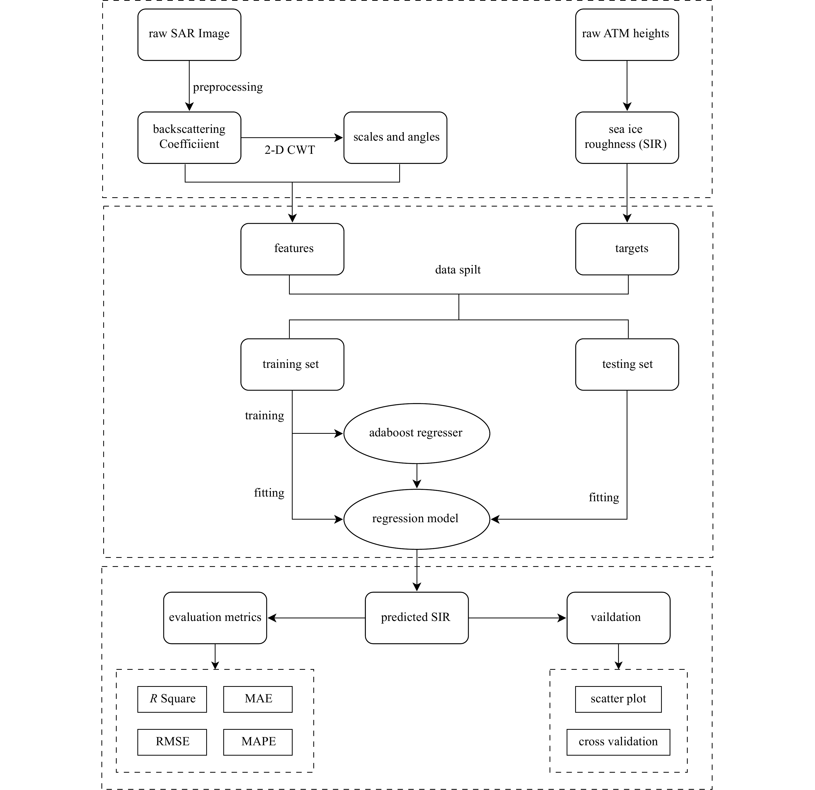
Abstract: Sea ice surface roughness (SIR) affects the energy transfer between the atmosphere and the ocean, and it is also an important indicator for sea ice characteristics. To obtain a small-scale SIR with high spatial resolution, a novel method is proposed to retrieve SIR from Sentinel-1 synthetic aperture radar (SAR) images, utilizing an ensemble learning method. Firstly, the two-dimensional continuous wavelet transform is applied to obtain the spatial information of sea ice, including the scale and direction of ice patterns. Secondly, a model is developed using the Adaboost Regression model to establish a relationship among SIR, radar backscatter and the spatial information of sea ice. The proposed method is validated by using the SIR retrieved from SAR images and comparing it to the measurements obtained by the Airborne Topographic Mapper (ATM) in the summer Beaufort Sea. The determination of coefficient, mean absolute error, root-mean-square error and mean absolute percentage error of the testing data are 0.91, 1.71 cm, 2.82 cm and 36.37%, respectively, which are reasonable. Moreover, K-fold cross-validation and learning curves are analyzed, which also demonstrate the method's applicability in retrieving SIR from SAR images.
-
Key words:
- 2-D Cauchy CWT /
- Adaboost Regression /
- sea ice /
- sea ice surface roughness
-

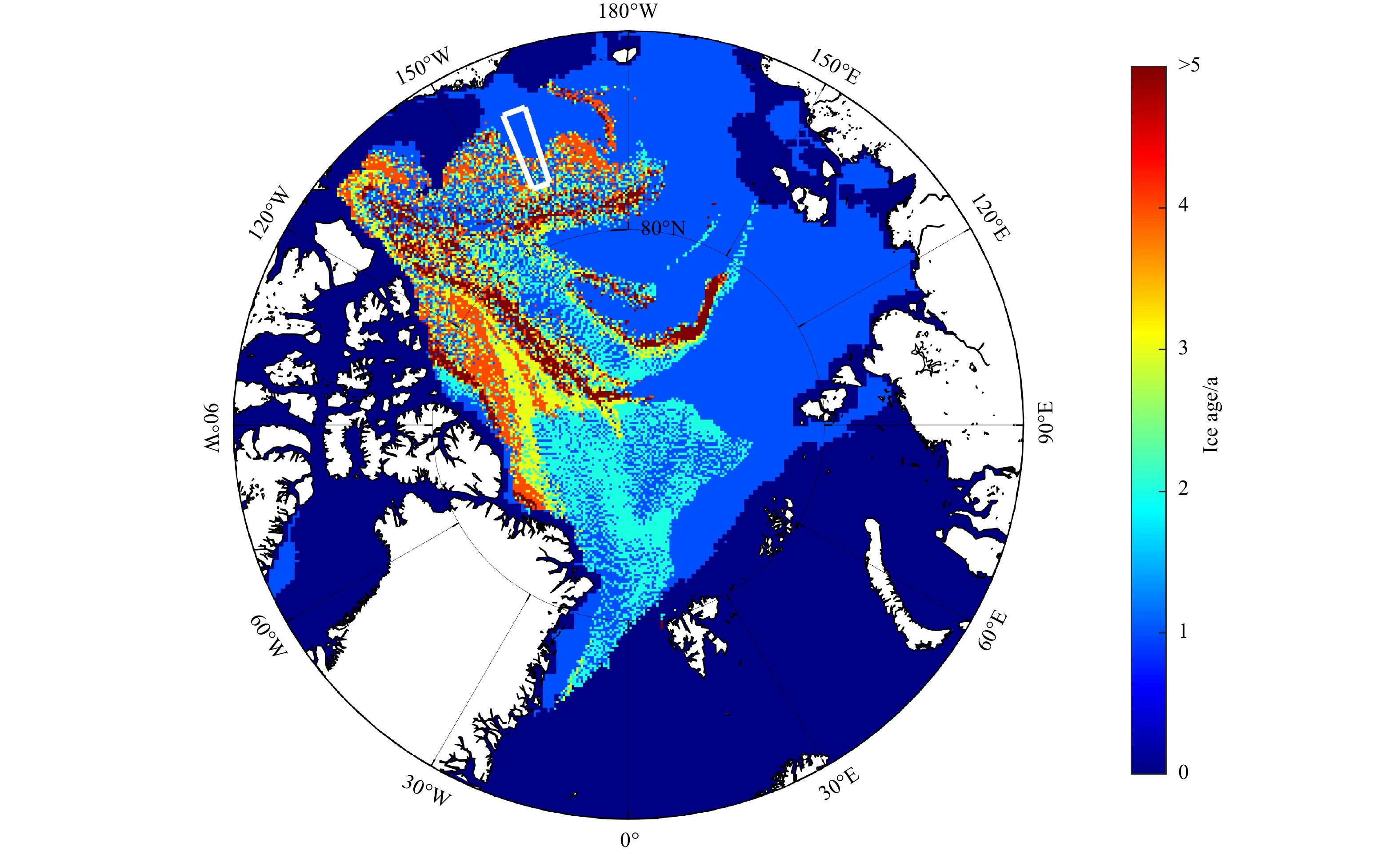
Figure 1. Map of the sea ice age from National Snow and Ice Data Center (NSIDC) (Tschudi et al., 2019) on July 15, 2016. Location of the study area is denoted as a white rectangle.

Figure 2. Preprocessed Sentinel-1 SAR image in HH-polarization sensed on July 13, 2016.

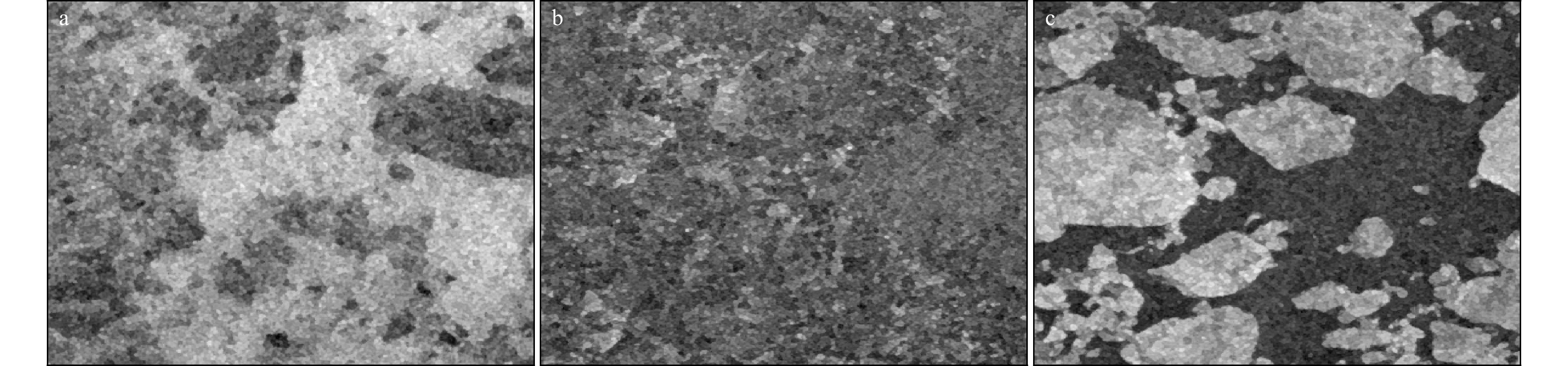
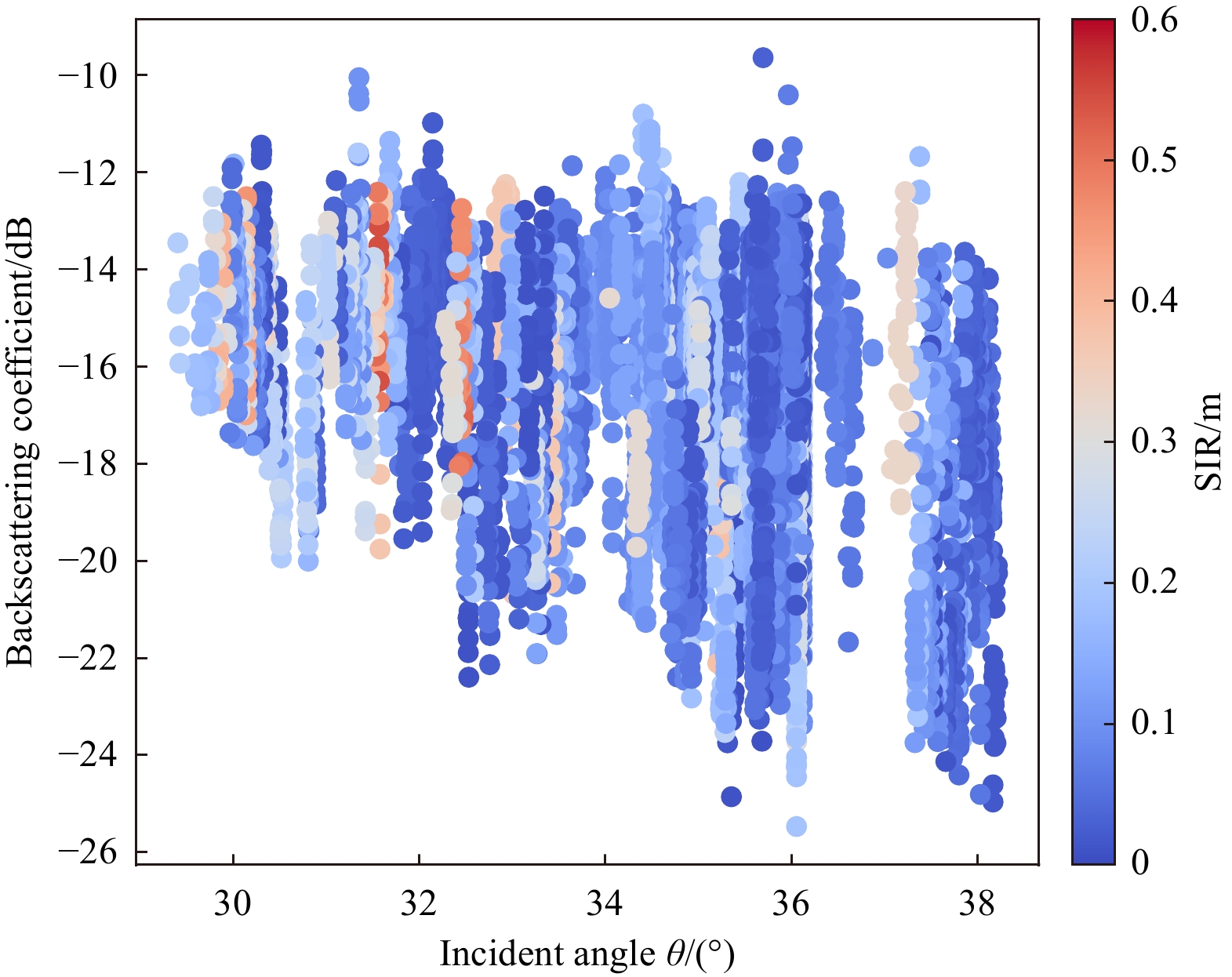
Figure 3. Sentinel-1 SAR HH-polarization backscatter coefficient (σ0) image under different incidence angles. a. Small incidence angle. b. Middle incidence angle. c. Large incidence angle.
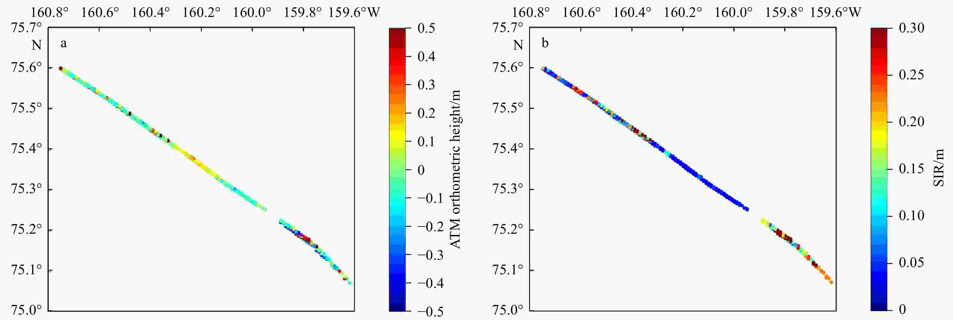
Figure 4. Spatial distribution of orthometric height and SIR in OIB ATM data. a. ATM orthometric height. b. Surfuce ice roughness.

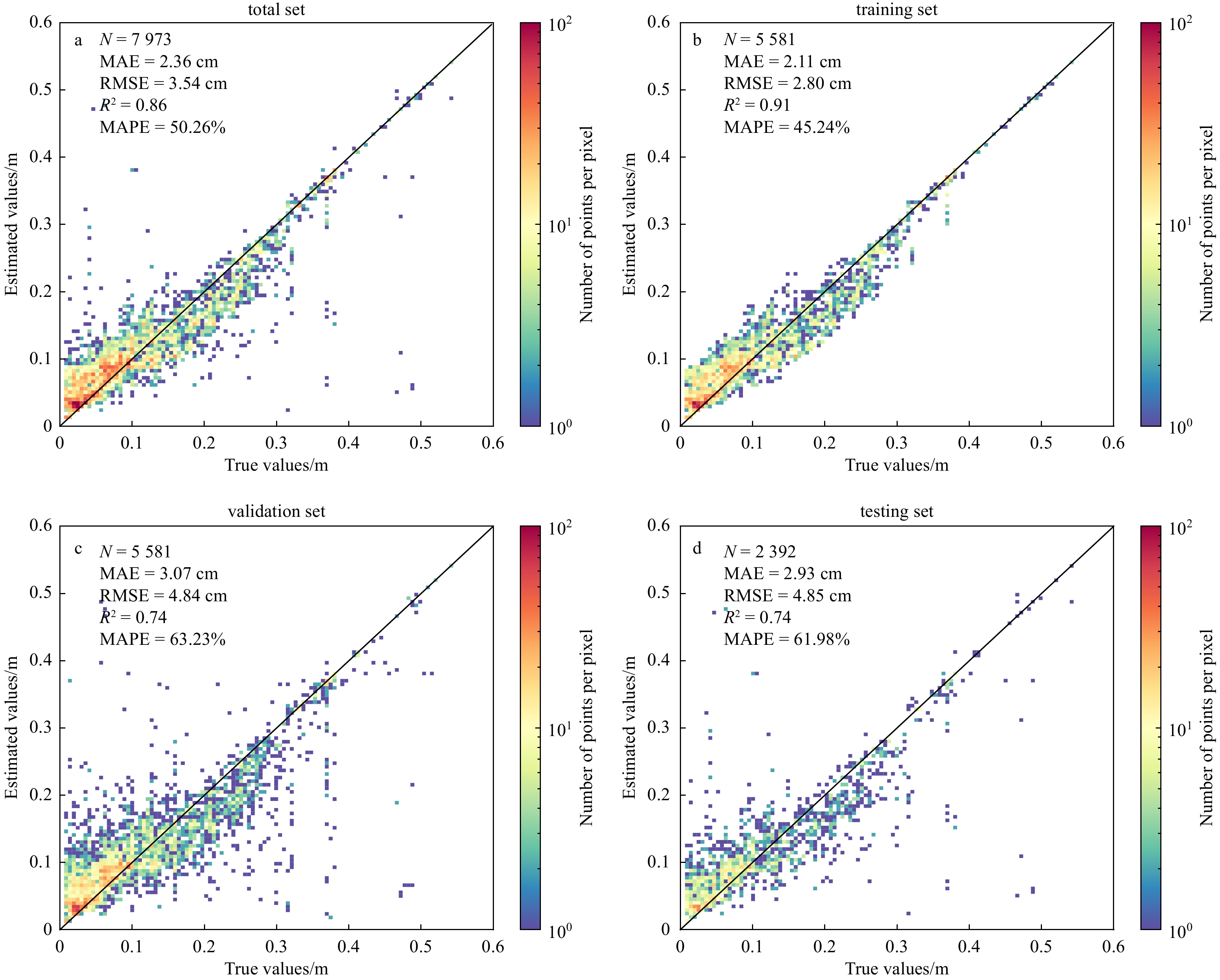
Figure 7. Scatter plots of the SIR measured by ATM and that estimated from SAR pixels.
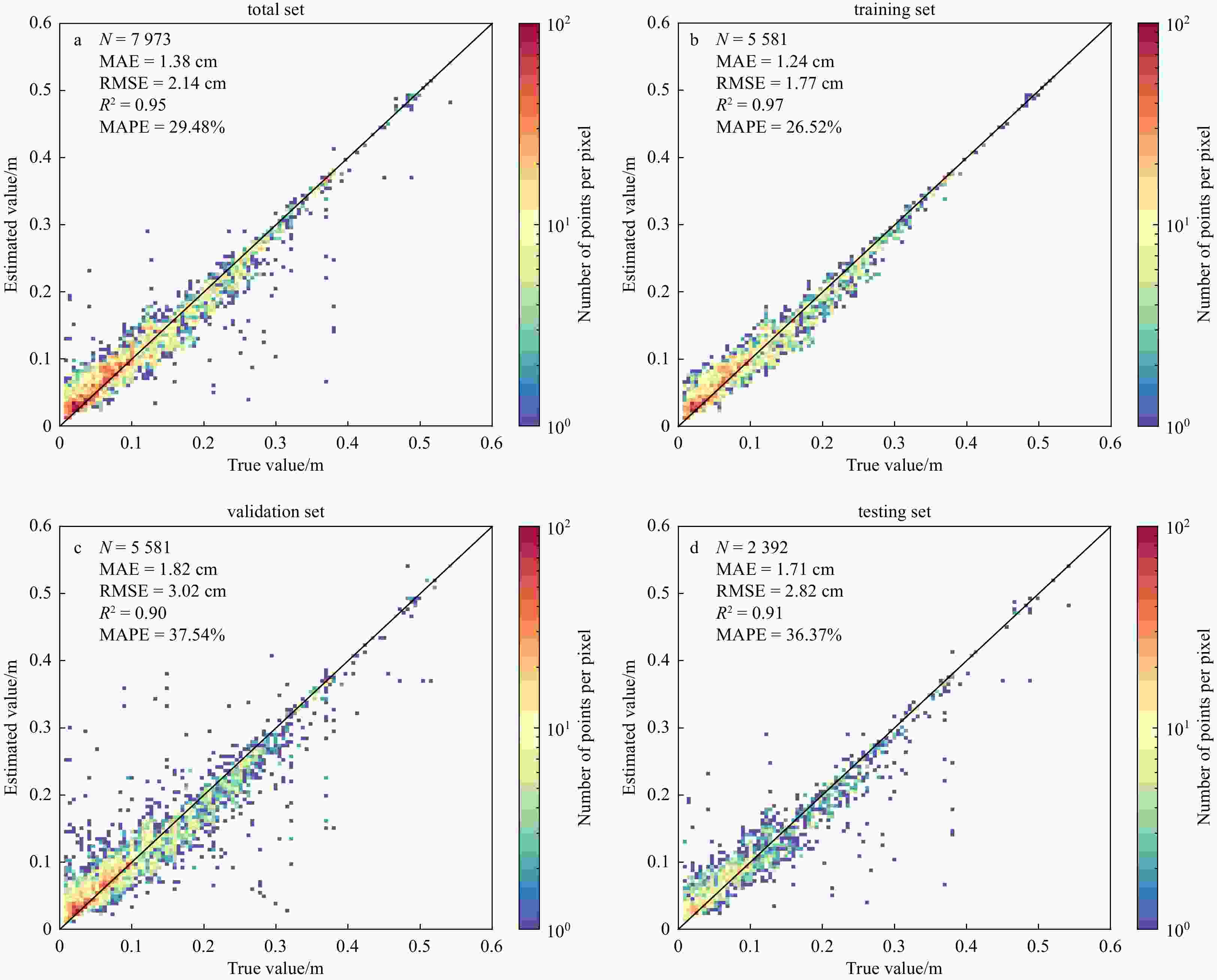
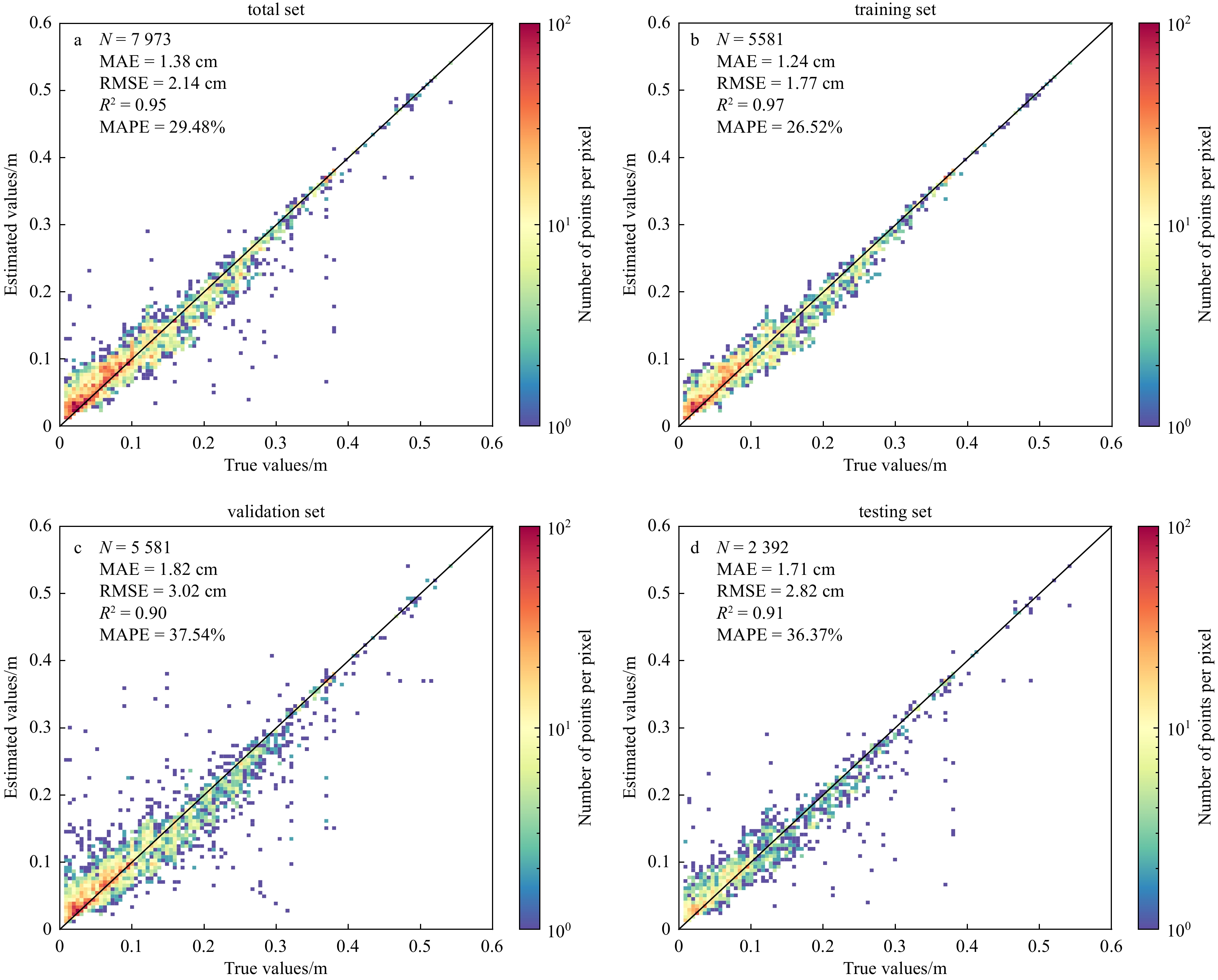
Figure 8. Scatter plots of the SIR measured by ATM and that estimated from SAR with 2-D CWT.
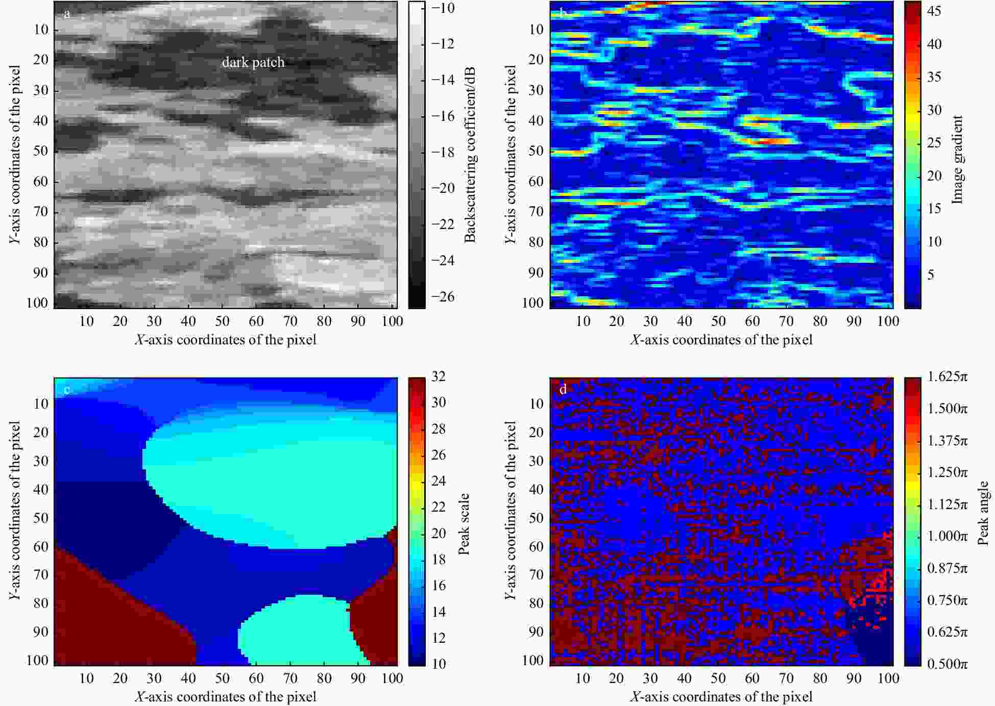
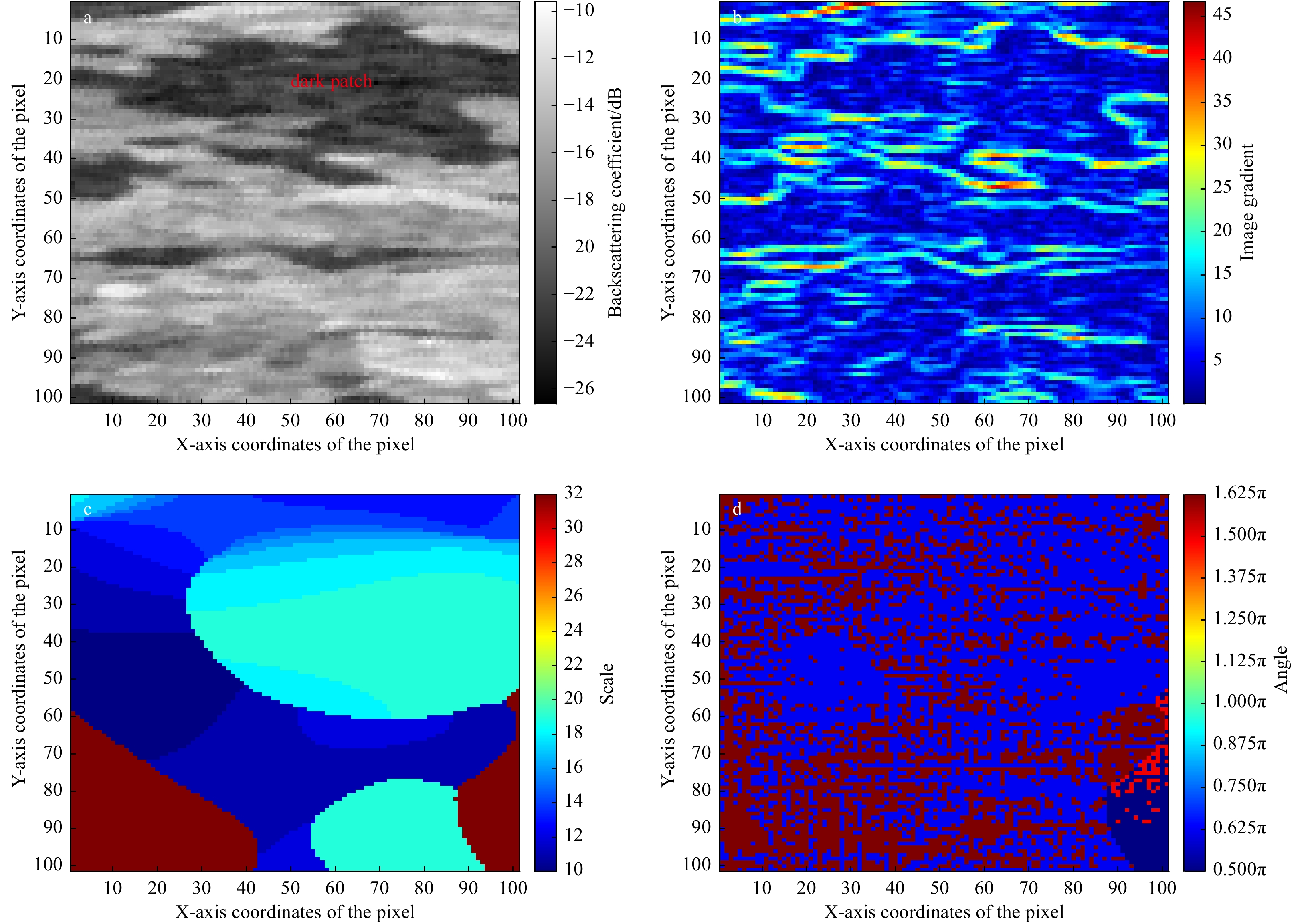
Figure 9. Results of 2-D Cauchy CWT. a. Region with ice floes (Area 4 in Fig. 2). b. Gradient of Fig. 9a. (c) Peak scales. (d) Peak angles.
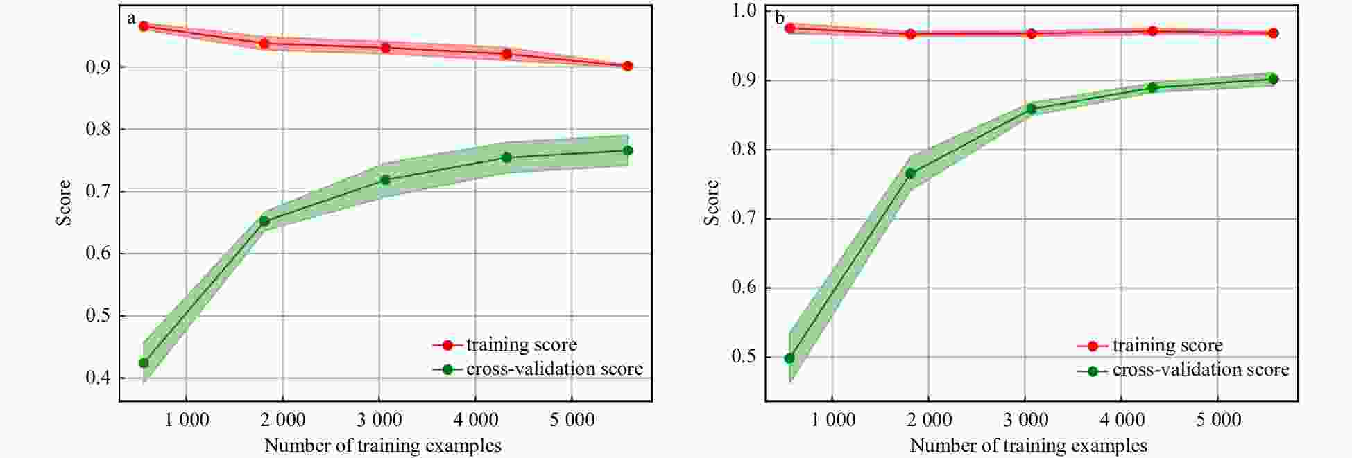
Figure 10. Learning curves for different types of input data. Input data without 2-D CWT (a) and input data with 2-D CWT (b). The score chosen is the coefficient of determination R2. The highlighted regions demonstrate 1 standard deviation error from the mean score of each fold.
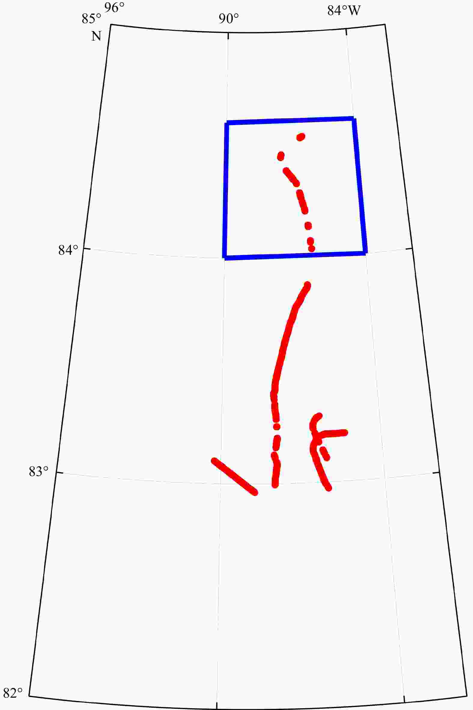
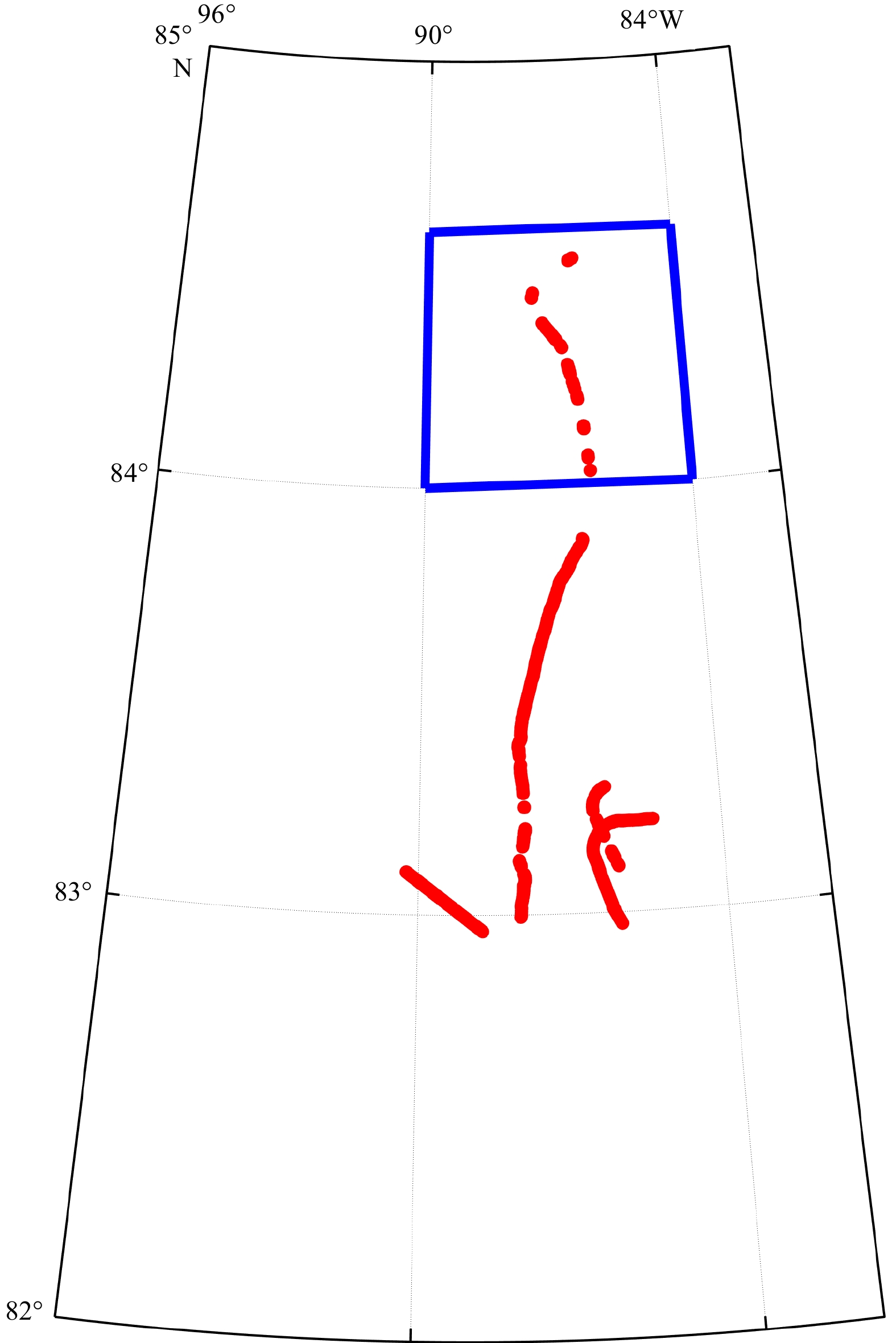
Figure 11. The spatial distribution of samples in Center Arctic. Location of the independent test area is denoted as a blue rectangle.
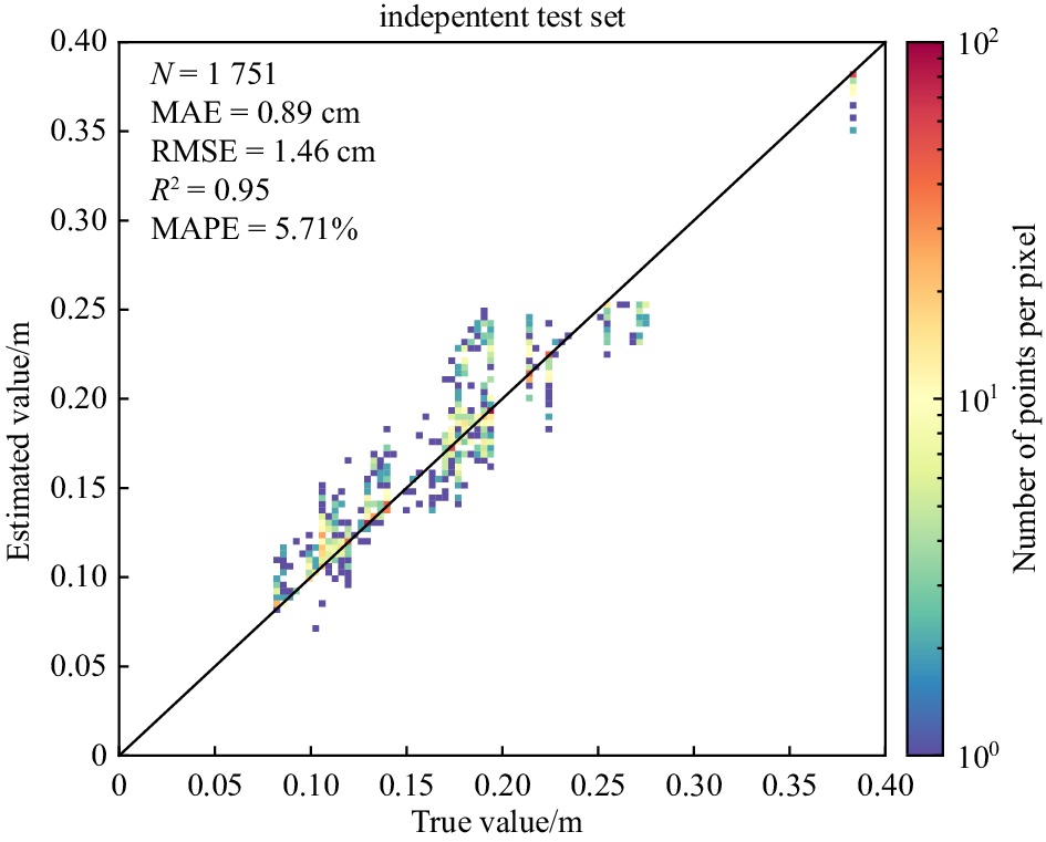
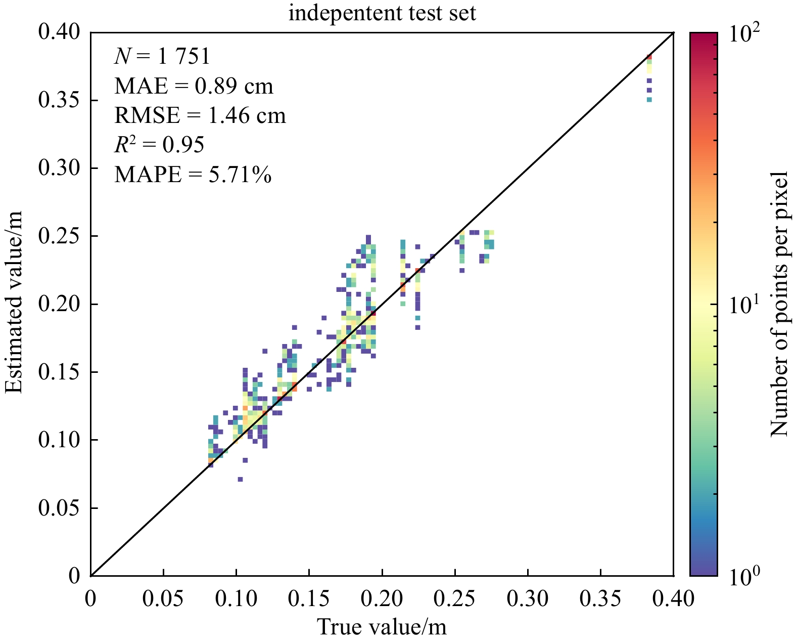
Figure 12. Scatter plots of the SIR in independent test region measured by ATM and that estimated from SAR with 2-D CWT.
Table 1. Sentinel-1 SAR images used in the study
Image id Product level Instrument mode Product type Longitude range Latitude range 1 L1 EW GRD 142.43°–166.67°W 75.72°–80.73°N 2 L1 EW GRD 151.74°–169.52°W 72.40°–76.99°N Resolution Polarisation Sensing start time Relative orbit number Incidence angle range Elevation angle range Medium HH, HV 17:46:09 161 19.10°–46.43° 17.12°–40.69° Medium HH, HV 17:47:13 161 19.19°–46.51° 17.20°–40.76°  下载: 导出CSV
Table 2. Value of 2-D Cauchy Wavelet Parameters
Parameter Default value A 1 $\alpha $ π/6 L 4 M 4
下载: 导出CSV
Algorithm1 Adaboost Regression Input: Training set $D = ({\vec x_i},{y_i})$, $i = 1,...,m$; $T$: Number of iterations; $I$: Weak learner;$L$: Loss function.
Output: Strong learner $H(\vec x) = \sum\limits_{i = 1}^T {\ln (\frac{1}{{{w_t}}})f(\vec x)} $
Initialization each sample’s weight of 1st iteration
for $i = 1$to $m$ do
$Dis{t_1}({\vec x_i}) \leftarrow 1/m$
end for
Training process
for $t = 1$to $T$ do
Training weak learner ${h_t} \leftarrow I(D,Dis{t_t})$
for $i = 1$to $m$ do
Updating maximum error ${E_t} \leftarrow max({E_t},L({y_i},{\vec x_i}))$
Calculating relative error for each sample ${e_{ti}} \leftarrow L({y_i},{\vec x_i})/{E_t}$
end for
Calculating error rate ${e_t} \leftarrow \sum\limits_{i = 1}^T {Dis{t_t}({{\vec x}_i}){e_{ti}}} $
Updating each learner's weight ${w_t} \leftarrow {e_t}/(1 - {e_t})$
for $i = 1$to $m$ do
Updating each learner’s weight $Dis{t_{t + 1}}({\vec x_i}) \leftarrow Dis{t_t}({\vec x_i})w_t^{1 - {e_{ti}}}$
end for
Normalize $Dis{t_t}({\vec x_i})$to be a proper distribution
$t = t + 1$
end for
Calculating the median of weighted predicted (${w_t}{h_t}$) value$f(\vec x)$
下载: 导出CSV
Table 3. Model evaluation metrics
Metric Formula Coefficient of determination (R2) $ R^2=1-\displaystyle\frac{\displaystyle\sum_{i=1}^N(\hat{y}_i-y_i)}{\displaystyle\sum^N_{i=1}(y_i-\bar{y})^2}$ Mean absolute error (MAE) $ MAE=\displaystyle\frac{1}{N}\sum^N_{i=1}|\hat{y}_i-y_i|$ Root mean square error (RMSE) $ RMSE=\sqrt{\displaystyle\frac{1}{N}\sum^N_{i=1}(\hat{y}_i-y_i)^2}$ Mean absolute percentage
error (MAPE)$ MAPE=\displaystyle\frac{1}{N}\sum^N_{i=1}\left|\frac{\hat{y}_i-y_i}{y_i}\right|\times 100\%$ Note: N is the size of dataset, $ \hat y_i$ is the predicted value, yi is the true value and $ \bar y$ represents the average of true values.
下载: 导出CSV
Table 4. Performance metrics of training and testing set
Dataset R2 MAE/cm RMSE/cm MAPE/% Training 0.91 2.11 2.8 45.24 Testing 0.74 2.93 4.85 61.98
下载: 导出CSV
Table 5. Performance metrics of each fold and average performance for the selected model
Fold MAE/cm RMSE/cm R2 MAPE/% 1 2.94 4.36 0.79 59.00 2 2.84 4.39 0.79 61.50 3 3.04 4.60 0.77 65.45 4 3.07 4.41 0.79 59.77 5 2.98 4.76 0.75 61.04 2.97 4.51 0.78 61.35 Note: The bold values are mean values.
下载: 导出CSV
Table 6. Performance metrics of training and testing set with 2-D CWT
Dataset R2 MAE/cm RMSE/cm MAPE/%z Training 0.97 1.24 1.77 26.52 Testing 0.91 1.71 2.82 36.37
下载: 导出CSV
Table 7. Performance of Each Fold and the Mean Value of Each Metric with 2-D CWT
Fold MAE/cm RMSE/cm R2 MAPE/% 1 1.77 3.04 0.90 33.41 2 1.84 2.64 0.92 40.77 3 1.66 2.63 0.92 36.07 4 1.81 3.03 0.90 38.04 5 1.73 2.90 0.91 36.20 1.76 2.86 0.91 36.90 Note: The bold values are mean values.
下载: 导出CSV
Table 8. Sentinel-1 SAR images used in the independent test
Image id Product level Instrument mode Product type Longitude range Latitude range 1 L1 EW GRD 58.89°–103.19°W 80.92°-86.11°N 2 L1 EW GRD 51.28°–97.67°W 81.27°–86.45°N 3 L1 EW GRD 60.61°–107.35°W 81.36°–86.54°N Resolution Polarisation Sensing start time Relative orbit number Incidence angle range Elevation angle range Medium HH, HV July 16, 2017 13 18.80°–46.66° 16.86°–40.89° Medium HH, HV July 17, 2017 13 18.95°–46.66° 16.99°–40.88° Medium HH, HV July 19, 2017 13 19.19°–46.47° 17.20°–40.72°
下载: 导出CSV
Table 9. Performance metrics of training and independent testing set
Dataset R2 MAE/cm RMSE/cm MAPE/% Training 0.97 1.31 1.92 10.17 Independent test 0.95 0.89 1.46 5.71
下载: 导出CSV
-
Antoine J P, Murenzi R. 1996. Two-dimensional directional wavelets and the scale-angle representation. Signal Processing, 52(3): 259–281. doi: 10.1016/0165-1684(96)00065-5 Antoine J P, Murenzi R, Vandergheynst P. 1999. Directional wavelets revisited: Cauchy wavelets and symmetry detection in patterns. Applied and Computational Harmonic Analysis, 6(3): 314–345. doi: 10.1006/acha.1998.0255 Babb D G, Landy J C, Barber D G, et al. 2019. Winter sea ice export from the Beaufort Sea as a preconditioning mechanism for enhanced summer melt: A case study of 2016. Journal of Geophysical Research: Oceans, 124(9): 6575–6600. doi: 10.1029/2019JC015053 Beckers J F, Renner A H H, Spreen G, et al. 2015. Sea-ice surface roughness estimates from airborne laser scanner and laser altimeter observations in Fram Strait and north of Svalbard. Annals of Glaciology, 56(69): 235–244. doi: 10.3189/2015AoG69A717 Cafarella S M, Scharien R, Geldsetzer T, et al. 2019. Estimation of level and deformed first-year sea ice surface roughness in the Canadian Arctic archipelago from C- and L- band synthetic aperture radar. Canadian Journal of Remote Sensing, 45(3-4): 457–475. doi: 10.1080/07038992.2019.1647102 Carlström A. 1997. A microwave backscattering model for deformed first-year sea ice and comparisons with SAR data. IEEE Transactions on Geoscience and Remote Sensing, 35(2): 378–391. doi: 10.1109/36.563277 Carlström A, Ulander L M H, Hakansson B. 1994. Model for estimating surface roughness of level and ridged sea ice using ERS-1 SAR. In: 1994 IEEE International Geoscience and Remote Sensing Symposium. Pasadena, CA,USA: IEEE,168–170 Daubechies I. 1992. Ten Lectures on Wavelets. Philadelphia, PA: Society for Industrial and Applied Mathematics Drucker H. 1997. Improving regressors using boosting techniques. In: Proceedings the 14th International Conference on Machine Learning. Nashiville: Morgan Kaufmann Publishers Inc. , 107–115 Efendi A, Fitriani R, Naufal H I, et al. 2020. Ensemble Adaboost in classification and regression trees to overcome class imbalance in credit status of bank customers. Journal of Theoretical and Applied Information Technology, 98(17): 3428–3437 Filipponi F. 2019. Sentinel-1 GRD preprocessing workflow. Proceedings, 18(1): 11 Grenfell T C, Perovich D K. 1984. Spectral albedos of sea ice and incident solar irradiance in the southern Beaufort Sea. Journal of Geophysical Research: Oceans, 89(C3): 3573–3580. doi: 10.1029/JC089iC03p03573 Gu Xiaowei, Angelov P P. 2022. Multiclass fuzzily weighted adaptive-boosting-based self-organizing fuzzy inference ensemble systems for classification. IEEE Transactions on Fuzzy Systems, 30(9): 3722–3735. doi: 10.1109/TFUZZ.2021.3126116 Gupta M, Barber D G. 2015. Sub-pixel evaluation of sea ice roughness using AMSR-E data. International Journal of Remote Sensing, 36(3): 749–763. doi: 10.1080/01431161.2014.1001081 Hong S. 2010. Detection of small-scale roughness and refractive index of sea ice in passive satellite microwave remote sensing. Remote Sensing of Environment, 114(5): 1136–1140. doi: 10.1016/j.rse.2009.12.015 Hsieh W W. 2023. Decision trees, random forests and boosting. In: Introduction to Environmental Data Science. Cambridge: Cambridge University Press, 473–493 Jackson C R, Apel J R. 2004. Synthetic Aperture Radar Marine User’s Manual. Washington, DC: National Oceanic and Atmospheric Administration, 377–379 Jiang Mingzhe, Clausi D A, Xu Linlin. 2022. Sea-ice mapping of RADARSAT-2 imagery by integrating spatial contexture with textural features. IEEE Journal of Selected Topics in Applied Earth Observations and Remote Sensing, 15: 7964–7977. doi: 10.1109/JSTARS.2022.3205849 Kim S H, Kim H C, Hyun C U, et al. 2020. Evolution of backscattering coefficients of drifting multi-year sea ice during end of melting and onset of freeze-up in the western Beaufort Sea. Remote Sensing, 12(9): 1378. doi: 10.3390/rs12091378 Landy J C, Petty A A, Tsamados M, et al. 2020. Sea ice roughness overlooked as a key source of uncertainty in CryoSat-2 ice freeboard retrievals. Journal of Geophysical Research: Oceans, 125(5): e2019JC015820. doi: 10.1029/2019JC015820 Lee J S, Jurkevich L, Dewaele P, et al. 1994. Speckle filtering of synthetic aperture radar images: A review. Remote Sensing Reviews, 8(4): 313–340. doi: 10.1080/02757259409532206 Li Xiaoming, Sun Yan, Zhang Qiang. 2021. Extraction of sea ice cover by Sentinel-1 SAR based on support vector machine with unsupervised generation of training data. IEEE Transactions on Geoscience and Remote Sensing, 59(4): 3040–3053. doi: 10.1109/TGRS.2020.3007789 Liu Mengjie, Dai Yongshou, Zhang Jie, et al. 2016. The microwave scattering characteristics of sea ice in the Bohai Sea. Acta Oceanologica Sinica, 35(5): 89–98. doi: 10.1007/s13131-016-0861-6 Marbouti M, Antropov O, Eriksson P, et al. 2018. Automated sea ice classification over the Baltic Sea using multiparametric features of Tandem-X InSAR images. In: 2018 IEEE International Geoscience and Remote Sensing Symposium. Valencia, Spain: IEEE,7328–7331 Martin T, Tsamados M, Schroeder D, et al. 2016. The impact of variable sea ice roughness on changes in Arctic Ocean surface stress: A model study. Journal of Geophysical Research: Oceans, 121(3): 1931–1952. doi: 10.1002/2015JC011186 Mohr F, van Rijn J N. 2022. Learning curves for decision making in supervised machine learning - A survey. arXiv: 2201.12150 Mosadegh E, Nolin A W. 2020. Estimating Arctic sea ice surface roughness by using back propagation neural network. In: AGU Fall Meeting 2020. San Francisco, CA,USA: AGU,C014–0005 Mosadegh E, Nolin A W. 2022. A new data processing system for generating sea ice surface roughness products from the multi-angle imaging spectroradiometer (MISR) imagery. Remote Sensing, 14(19): 4979. doi: 10.3390/rs14194979 Nolin A W, Mar E. 2018. Arctic sea ice surface roughness estimated from multi-angular reflectance satellite imagery. Remote Sensing, 11(1): 50. doi: 10.3390/rs11010050 Palerme C, Müller M. 2021. Calibration of sea ice drift forecasts using random forest algorithms. The Cryosphere, 15(8): 3989–4004. doi: 10.5194/tc-15-3989-2021 Pedregosa F, Varoquaux G, Gramfort A, et al. 2011. Scikit-learn: Machine learning in Python. Journal of Machine Learning Research, 12: 2825–2830 Prasad S, Haynes R D, Zakharov I, et al. 2021. Estimation of sea ice parameters using an assimilated sea ice model with a variable drag formulation. Ocean Modelling, 158: 101739. doi: 10.1016/j.ocemod.2020.101739 Segal R A, Scharien R K, Cafarella S, et al. 2020. Characterizing winter landfast sea-ice surface roughness in the Canadian Arctic archipelago using Sentinel-1 synthetic aperture radar and the multi-angle imaging spectroradiometer. Annals of Glaciology, 61(83): 284–298. doi: 10.1017/aog.2020.48 Shanmugasundar G, Vanitha M, Čep R, et al. 2021. A comparative study of linear, Random Forest and AdaBoost Regressions for modeling non-traditional machining. Processes, 9(11): 2015. doi: 10.3390/pr9112015 Studinger M. 2014. IceBridge ATM l2 Icessn elevation, slope, and roughness, version 2. NASA National Snow and Ice Data Center Distributed Active Archive Center. https://nsidc.org/data/ILATM2/versions/2 [2023-06-01 Torres R, Snoeij P, Geudtner D, et al. 2012. GMES Sentinel-1 mission. Remote Sensing of Environment, 120: 9–24. doi: 10.1016/j.rse.2011.05.028 Tschudi M, Meier W N, Stewart J S, et al. 2019. EASE-grid sea ice age, version 4. NASA National Snow and Ice Data Center Distributed Active Archive Center. https://nsidc.org/data/NSIDC-0611/versions/4 [2023-06-01 Wen Xiaoyang, Xue Cunjin, Dong Qing. 2011. The Arctic sea ice surface roughness estimation and application. In: Proceedings of the 21st International Offshore and Polar Engineering Conference. Maui, Hawaii,USA: ISOPE,958–961 Xiao Changjiang, Chen Nengcheng, Hu Chuli, et al. 2019. Short and mid-term sea surface temperature prediction using time-series satellite data and LSTM-AdaBoost combination approach. Remote Sensing of Environment, 233: 111358. doi: 10.1016/j.rse.2019.111358 Yan Qingyun, Huang Weimin. 2019. Detecting sea ice from TechDemoSat-1 data using Support Vector Machines with feature selection. IEEE Journal of Selected Topics in Applied Earth Observations and Remote Sensing, 12(5): 1409–1416. doi: 10.1109/JSTARS.2019.2907008 Zhu Zonghai, Wang Zhe, Li Dongdong, et al. 2020. Geometric structural ensemble learning for imbalanced problems. IEEE Transactions on Cybernetics, 50(4): 1617–1629. doi: 10.1109/TCYB.2018.2877663 -


 点击查看大图
计量
- 文章访问数: 115
- HTML全文浏览量: 51
- 被引次数: 0

