

Wave hindcast under tropical cyclone conditions in the South China Sea: sensitivity to wind fields
-
Abstract: Reliable wave information is critical for marine engineering. Numerical wave models are useful tools to obtain wave information with continuous spatiotemporal distributions. However, the accuracy of model results highly depends on the quality of wind forcing. In this study, we utilize observations from five buoys deployed in the northern South China Sea from August to September 2017. Notably, these buoys successfully recorded wind field and wave information during the passage of five tropical cyclones of different intensities without sustaining any damage. Based on these unique observations, we evaluated the quality of four widely used wind products, namely CFSv2, ERA5, CCMP, and ERAI. Our analysis showed that in the northern South China Sea, ERA5 performed best compared to buoy observations, especially in terms of maximum wind speed values at 10 m height (U10), extreme U10 occurrence time, and overall statistical indicators. CFSv2 tended to overestimate non-extreme U10 values. CCMP showed favorable statistical performance at only three of the five buoys, but underestimated extreme U10 values at all buoys. ERAI had the worst performance under both normal and tropical cyclone conditions. In terms of wave hindcast accuracy, ERA5 outperformed the other reanalysis products, with CFSv2 and CCMP following closely. ERAI showed poor performance especially in the upper significant wave heights. Furthermore, we found that the wave hindcasts did not improve with increasing spatiotemporal resolution, with spatial resolution up to 0.5°. These findings would help in improving wave hindcasts under extreme conditions.
-
Key words:
- wave hindcast /
- SWAN /
- tropical cyclone /
- South China Sea
-
1. Introduction
Wind-induced surface waves are crucial for navigation, ocean engineering, and physical oceanography (Weintrit, 2009). Numerical models are helpful and widely used tools that can provide a wide range of continuous spatiotemporal wave information (Lavrenov, 2003). However, it is generally recognized that the reliability of model results depend on the quality of the wind field input (Jun et al., 2015; Chalikov, 2018). Wind products provided by different agencies with different spatiotemporal resolutions may produce different simulation results, which leads to uncertainties in the use of simulated wave parameters in ocean engineering (Qiao et al., 2019).
There are many widely used and easily accessible wind products, such as those from the National Centers for Environmental Prediction (NCEP), European Centre for Medium-Range Weather Forecasts (ECMWF), and Japan Meteorological Agency (JMA) (Kanwal et al., 2022; Van Vledder and Akpınar, 2015). In addition to differences in spatial and temporal resolution, the assimilation methods and assimilated observations are also very different, indicating that these wind products would perform differently under the local real wind field in a given region. These differences lead to large discrepancies in the output of wave models driven by wind fields (Chen et al., 2019).
To date, many evaluations of wind products have been conducted for different time periods and regions. Van Vledder and Akpınar (2015) evaluated the performance of six wind datasets for wave hindcasts in the Black Sea and found that the uncalibrated Climate Forecast System Reanalysis (CFSR) wind dataset performed best for both long periods and extreme conditions. Stopa (2018) compared the advantages and disadvantages of ten reanalysis wind datasets and two merged satellite observational datasets, as well as their performance in wave hindcasts in global waters, and provided recommendations on the most accurate wind datasets for wave hindcast generation. This study applies various metrics to evaluate the performance of wind and wave datasets with reference to synchronous observations and suggests the most appropriate recommendations for numerical simulations. However, the low spatiotemporal resolution of the datasets must be considered. Many studies, especially those related to climate change, use coarse resolution wind and wave datasets from Hybrid Coordinate Ocean Model (HYCOM), WAVEWATCH III (WW3), and ECMWF owing to limitations in computational resources (Morim et al., 2022; Wang et al., 2020). This makes it difficult to distinguish the wind and wave characteristics during extreme events such as tropical cyclone (TC) conditions. The simultaneous evaluation of the performance of different wind products and the variability in results generated by wind-field-driven wave models remains scarce, mainly because simultaneous observations of wave and wind fields are rare.
With the advancement of computational resources and observational technologies, such assessments are increasingly enriched and improved. In an evaluation of winds from ECMWF Reanalysis-Interim (ERAI) and ECMWF Reanalysis v5 (ERA5) (Becerra et al., 2022) suggested that ERA5 performs better in both deep and coastal waters along the Chilean coast. In addition, Gualtieri (2021) evaluated 15 reanalysis products at different locations and found ERA5 to be more reliable offshore.
The South China Sea (SCS) is the largest marginal sea in the northwestern Pacific Ocean and is an important shipping lane (Fig. 1). Owing to the lack of synchronous wind and wave observations, assessments of wind quality and wave hindcasts in the SCS are still limited. It remains unclear which wind products are more suitable for wave hindcasting in the SCS, especially under extreme conditions, and whether the spatiotemporal resolution of wind forcing is a main factor affecting wave hindcasts’ quality.
 Figure 1. The study area, bathymetry (color fill), and tracks of five tropical cyclone (TCs) during the study period. The magenta triangles represent buoy positions.
Fortunately, five buoys deployed in the northern SCS (Fig. 1) provide a relatively complete and simultaneous record of wind and wave parameters over a two-month period (August–September, 2017), during which four TCs of different intensities hit the northern SCS. This provided an excellent opportunity to simultaneously evaluate the performance of four widely used wind reanalysis datasets, particularly under TC conditions, and the variability of wave parameters simulated by these wind-product-driven wave models compared with observations. Furthermore, numerical experiments were designed to investigate the influence of wind forcing at different spatiotemporal resolutions. Our findings will allow researchers to quickly select the most ideal wind field to study waves in the SCS and will provide an important scientific basis for improving regional wave field prediction.
The remainder of this paper is organized as follows: Section 2 describes the wind datasets, observational data, and the implementation of the wave model. In Section 3, the wind data and their performance in wave hindcasts are evaluated, and the sensitivity of the spatial and temporal resolutions of the wind data in wave hindcasts is discussed. Finally, a summary and conclusions are presented in Section 4.
2. Data and methods
In this section, the datasets used in the present study and information on TCs are presented. A detailed description of the wave model implementation and numerical experiments is provided.
2.1 Wind products and observational data
Information on the five TCs that passed over the northern SCS during August-September, 2017, was obtained from the JMA (the track of each TC is shown in Fig. 1). The best track data from the JMA included the TC category, location, central pressure, wind direction, and time series of the longest and shortest radii with winds of 30 kn and 50 kn or more.
Four widely used wind products, namely ERAI, ERA5, CFSv2, and Cross-Calibrated Multiplatform (CCMP) are considered in this study. The spatiotemporal resolution of each wind dataset is presented in Table 1. ERAI is a reanalysis dataset provided by the ECMWF that uses an improved atmospheric model and assimilation system to replace the previous version, ERA-40 (Dee et al., 2011). The available data cover the years 1979–2019, with a temporal resolution of 3 h and a spatial resolution of 0.25°. ERA5 is the fifth generation ECMWF atmospheric reanalysis dataset (Hersbach et al., 2020). The ERA5 data cover the period from 1979 to the present and have the same spatiotemporal resolution as ERAI, but perform better in terms of precipitation distribution, sea surface temperature, and sea ice. By comparing ERA5 and ERAI, we assess whether the new generation of wind products is better than the previous generation, and in particular, if wave simulation is improved. The CFSv2 reanalysis wind data is the second version of the NCEP’s CFSR, and is available at horizontal resolutions of 0.25°, 0.5°, 1.0°, and 2.5° at hourly intervals (Saha et al., 2014). In this study, a horizontal resolution of 0.25° was selected. CCMP (Atlas et al., 1996, 2011; Hoffman et al., 2003) is a merged satellite wind analysis dataset. The satellite data include active instruments (scatterometers, QuickSCAT, and ASCAT) and passive microwave sensors (radiometers, SSM/I, SSMIS, TMI, GMI, AMSR2, AMSRE, and WindSat).
Table 1. Features of wind datasetsData source Temporal coverage Temporal resolution/h Spatial resolution ERAI 1979−2019 3 0.25° ERA5 1979−2021 3 0.25° CFSv2 2011−present 1 0.125° CCMP 1987−present 6 0.25° Note: ERAI: ECMWF Reanalysis-Interim; ERA5: ECMWF Reanalysis v5; CFSv2: NCEP Climate Forecast System Version 2; CCMP: Cross-Calibrated Multiplatform. | Show Table DownLoad:
CSV
DownLoad:
CSV
The observations were based on buoys operated by the Ministry of Natural Resources of China in the northern SCS (Fig. 1), specifically identified as Buoys B1−B5. The observational data started on August 1, 2017, and ended on September 30, 2017. The time interval between observations was 1 h. The observed parameters included wind speed, wind direction, significant wave height, wave direction, mean wave period, and peak wave period. The latitude and longitude of the buoys and the corresponding water depth are given in Table 2. Wind observed by the buoys was 4 m above the sea surface. To ensure consistency with the wind data sets, it is necessary to convert the observed wind speed to a height of 10 m above the sea surface. To extrapolate the surface wind speed, we used the method based on the Monin-Obukhov theory (Monin and Obhukov, 1954). Unfortunately, some buoy observations lacked the necessary friction velocity, temperature, and heat flux measurements. To overcome this limitation, Liu and Tang (1996) introduced a simplified exponential wind speed profile equation that allows atmospheric stability to be neglected. Previous studies have shown that the assumption of a neutral or stable atmosphere results in negligible differences in near-surface wind speeds, especially for small height differences such as 4 m to 10 m (Bourassa et al., 2003; Chelton and Freilich, 2005; Kara et al., 2008). This assumption has been successfully applied in many studies (Mears and Wentz, 2001; Ruti et al., 2008; Hawkins et al., 2011; Carvalho et al., 2014). Therefore, for this study, we adopted the power law formula proposed by Hawkins et al. (2011) as the simplified wind speed profile equation for extrapolating surface wind speeds.
Table 2. Features of buoysBuoy Latitude Longitude Depth/m Number of Samples B1 21.12°N 112.63°E 50.43 1468 B2 21.50°N 114.00°E 54.02 1478 B3 22.28°N 115.60°E 49.17 1635 B4 22.87°N 117.10°E 40.60 1172 B5 19.87°N 115.46°E 1243.69 1472 | Show TableDownLoad:
CSV
$$ {U}_{z}={U}_{m}\frac{{\rm{ln}}\left(z/{{z}}_{0}\right)}{{\rm{ln}}\left({z}_{m}/{{z}}_{0}\right)}, $$ (1) where
$ {U}_{z} $ represents to the wind speed at a desired measurement height z (z = 10).$ {U}_{m} $ represents to the wind speed at a reference height (z = 4).$ {z}_{0} $ is the roughness length and the typical oceanic value for$ {{z}}_{0} $ is 1.52 ×10⁻⁴ m (Peixoto and Oort, 1992).2.2 TCs in August-September, 2017, in the SCS
The five TCs’ tracks of interest are displayed in Fig. 1. TC Hato (1713) emerged as a tropical depression over the eastern Luzon Strait on August 19, 2017, and developed into a tropical storm the following day. On August 21, TC Hato emerged over the northern SCS and reached typhoon intensity. Rapid intensification ensued in TC Pakhar (1714), which followed TC Hato and was a strong tropical storm that hit southern China in late August. Pakhar developed from a tropical depression east of Luzon Strait on August 24, and intensified into a tropical storm later that day. Pakhar made its first landfall over the Philippines on August 25, and then moved into the SCS, gradually increasing in intensity. It peaked as a severe tropical storm on August 27 and made its second landfall over the coast of Guangdong Province. On August 30, TC Mawar (1716) developed as a tropical depression over the northeastern Luzon Strait and intensified into a severe tropical storm early on September 2. By September 3, TC Mawar weakened into a tropical storm and made landfall over southeastern China late in the day. TC Guchol (1717) formed as a tropical depression over the Luzon Strait early on September 6 and generally moved north-northwest. It peaked in intensity in the afternoon, with an estimated sustained wind of 55 km/h, and degenerated into a depression over the Taiwan Strait the following day. TC Doksuri (1719) developed as a weak tropical depression east of the Philippines on September 10. On September 13, after entering the SCS, Doksuri intensified into a severe tropical storm. One day later, it further intensified to a Category 2 typhoon and made landfall in Vietnam with a peak intensity on September 15.
In the following sections, we will divide the period of interest into three segments: the entire period, the TC-only period, and the TC-free period. The full period is from August 1, 2017 to September 30, 2017. The TC-only period includes the entire period from the formation to the dissipation of five TCs, according to the information provided by the JMA. These TCs include TC Hato from 12:00 am on August 19 to 00:00 am on August 25, TC Pakhar from 00:00 am on August 24 to 00:00 am on August 28, TC Mawar from 6:00 am on August 30 to 6:00 am on September 4, TC Guchol from 12:00 am on September 3 to 12:00 am on September 7, and TC Doksuri from 00:00 am on September 10 to 00:00 am on September 16. The TC-free period refers to the remaining period obtained by subtracting the above five TC periods from the total period.
2.3 Wave model description
The wave hindcast was performed using the third-generation wave model, Simulating Waves Nearshore (SWAN, v41.31, Booij et al., 1999). The physical processes of waves, including wave generation and propagation, three- and four-wave interactions, whitecapping, wave dissipation, transmission, and diffraction, are described based on the dynamic spectral balance equation given:
$$ \frac{\partial }{\partial t}N+\frac{\partial }{\partial x}{C}_{x}N+\frac{\partial }{\partial y}{C}_{y}N+\frac{\partial }{\partial \sigma }{C}_{\sigma }N+\frac{\partial }{\partial \theta }{C}_{\theta }N=\frac{{S}_{{\rm{tot}}}}{\sigma }, $$ (2) $$ N=\frac{E}{\sigma }, $$ (3) where N
$ \left(\sigma ,\theta ,x,y,t\right) $ represents the wave action spectrum, E$ \left(\sigma ,\theta \right) $ represents the wave energy spectrum,$ \sigma $ is the relative frequency,$ \theta $ is the wave propagation direction.$\dfrac{\partial }{\partial x}{C}_{x}N$ ,$\dfrac{\partial }{\partial y}{C}_{y}N$ ,$\dfrac{\partial }{\partial \sigma }{C}_{\sigma }N$ and$\dfrac{\partial }{\partial \theta }{C}_{\theta }N$ are the propagations of the wave action spectrum in spatialal space (x, y) and spactral space ($ \sigma $ ,$ \theta $ ), respectively.${S}_{{\rm{tot}}}$ is the total source term, which is composed of wind energy input${S}_{{\rm{in}}}$ , three-wave interactions${S}_{{\rm{nl3}}}$ , four-wave interactions${S}_{{\rm{nl4}}}$ , whitecapping dissipation${S}_{{\rm{ds}},{\rm{w}}}$ , bottom friction${S}_{{\rm{ds}},{\rm{b}}}$ , and depth-induced friction${S}_{{\rm{ds}},{\rm{br}}}$ :$$ {S}_{{\rm{tot}}}={S}_{{\rm{in}}}+{S}_{{\rm{nl3}}}+{S}_{{\rm{nl4}}}+{S}_{{\rm{ds,w}}}+{S}_{{\rm{ds,b}}}+{S}_{{\rm{ds,br}}}. $$ (4) The input wind field mainly affected
$ {S}_{{\rm{in}}} $ and$ {S}_{{\rm{ds,w}}} $ . The source terms can be formulated as:$$ {S}_{{\rm{in}}}\left(\sigma ,\theta \right)=A+BE(\sigma ,\theta ), $$ (5) $$ {S}_{{\rm{ds,w}}}\left(\sigma ,\theta \right)=-{\varGamma }\tilde{\sigma }\frac{k}{\tilde{k}}E(\sigma ,\theta ) ,$$ (6) where A is given by Cavaleri and Rizzoli (1981) and B is formulated by Snyder et al. (1981) and Janssen (1989).
$ {\varGamma } $ is the coefficient depending on steepness, k is the wave number, and$ \tilde{\sigma } $ and$ \tilde{k} $ are the mean frequency and mean wave number, respectively.2.4 Model setup and configuration
The model domain covers the entire SCS (Fig. 1) with a spatially variable grid resolution ranging from 1.3 km in the nearshore region of the northern SCS to 15 km in the open water region. Horizontal coordinates (x, y) were arranged as a 967 × 653 array, and bathymetric data from the General Bathymetric Chart of the Ocean were interpolated into the model grid. The wave spectrum consisted of 36 directions and 24 frequencies ranging from 0.04 Hz to 1 Hz. Whitecapping was simulated using a scheme proposed by Komen et al. (1984). Quadruplet interactions were estimated using the discrete interaction approximation from Hasselmann et al. (1985). The depth-induced breaking from Battjes and Janssen (1978) and bottom friction formulation from Hasselmann et al. (1973) were also chosen. A numerical propagation scheme of the backward space and backward time (BSBT) was used. Boundary forcing was provided by a 2D spectrum from a global wave hindcast performed by the WW3 wave model. The model was sequentially forced with the five wind fields mentioned above, with initial conditions set to 0. The total run time was from August 1 to September 30, 2017, with a time step of 300 s. The significant wave height, peak wave period, and wave direction were output every hour of the analysis.
2.5 Metric indicators
To accurately assess the performance of the wind data and wave hindcasts, five widely used metric indicators were applied in this study: relative standard deviation (STD), root mean square error (RMSE), correlation coefficient (
$ {r}^{2} $ ), BIAS, and scatter index (SI). STD represents the divergence of the data. RMSE reflects the precision of the estimated values.$ {r}^{2} $ reflects the degree of correlation between the four wind data points and observations (Taylor, 2005). BIAS measures the average difference between the estimated values and observations. The SI is the normalized measure of error. These definitions are as follows:$$ {\rm{STD}} =\frac{\sqrt{\displaystyle\frac{1}{N}\sum_{i=1}^{N}{{(p}_{i}-\bar{p})}^{2}}}{\bar{o}}, $$ (7) $${\rm{ RMSE}}=\sqrt{\frac{1}{N}\sum _{i=1}^{N}{({p}_{i}-{o}_{i})}^{2}} ,$$ (8) $$ {r}^{2}=\frac{\displaystyle\sum _{i=1}^{N}({p}_{i}-\bar{p})({o}_{i}-\bar{o})}{\sqrt{\displaystyle\sum _{i=1}^{N}{\left({p}_{i}-\bar{p}\right)}^{2}{({o}_{i}-\bar{o})}^{2}}} ,$$ (9) $$ {\rm{BIAS}}=\frac{\displaystyle\sum _{i=1}^{N}({p}_{i}-{o}_{i})}{N}, $$ (10) $$ {\rm{SI}}=\frac{{\rm{RMSE}}}{\bar{o}} ,$$ (11) where
$ {p}_{i} $ is the estimated value,$ {o}_{i} $ the observed value, and N the number of samples.3. Results and discussion
In this study, the quality of the four wind datasets between August 1 and September 30, 2017 was evaluated. The wave hindcasts sequentially forced by the four wind datasets were also evaluated. Furthermore, the influence of the input wind data with different spatiotemporal resolutions on the wave hindcast was assessed.
3.1 Wind product assessment
The wind speed and direction time series obtained from the four wind datasets (ERAI, ERA5, CCMP, and CFSv2) were compared with the buoy observations, as shown in Fig. 2. All wind fields showed similar variations and magnitudes, which indicated that the four wind products sufficiently captured the overall evolution of the observed wind speed and direction. During all TCs except TC Guchol, there were extreme wind speeds at 10 m (U10) and notable changes in wind direction; however, the peaks of each U10 varied from buoy to buoy and occurred at different times (Table 3), mainly because of the positions of each buoy relative to the different TC tracks. Among the four wind products, the maximum U10 of CFSv2 at Buoys B1–B4 and the maximum U10 of ERA5 at B5 were closest to the observations. The maximum and mean U10 values of CCMP and ERAI were significantly smaller than the values observed in TC-only period. The discrepancy between the maximum U10 of ERAI and observations reached up to 31.31 m/s. Regarding the time of occurrence of the maximum U10, ERA5 was closest to the observation at all buoys, while ERAI and CCMP had time lags at Buoys B1–B4, which may be due to their coarse temporal resolution. From the visual comparison described above, we concluded that CCMP and ERAI underestimated U10 in TC-only period, while ERA5 and CFSv2 showed better performance, and ERA5 estimated the maximum U10 occurrence time most accurately.
 Figure 2. Time series of U10 (wind speed at 10 m height), wind direction between four wind data and corresponding buoy observations, with the time period from August 1 to September 30, 2017. The five periods of tropical cyclone (TC) occurrences are marked with a semi-transparent background color, from left to right: TC Hato, TC Pakhar, TC Mawar, TC Guchol, TC Doksuri. CCMP: Cross-Calibrated Multiplatform; ERAI: ECMWF Reanalysis-Interim; ERA5: ECMWF Reanalysis v5; CFSv2: NCEP Climate Forecast System Version 2; OBS: buoy observation.Table 3. Average value (mean), maximum value of wind speed at 10 m height (U10) of the four wind data and corresponding hour when reaching the maximum value during each tropical cyclone period
Mean U10/(m·s−1) Maximum U10/(m·s−1) Occurrence of maximum U10/h Hato Pakhar Mawar Guchol Doksuri Hato Pakhar Mawar Guchol Doksuri Hato Pakhar Mawar Guchol Doksuri Buoy B1 6.67 7.20 3.38 3.26 6.25 18.60 15.20 7.40 11.10 16.60 92 64 113 33 104 CCMP 5.71 6.85 2.91 2.97 5.67 12.96 9.77 7.37 4.39 12.46 91 67 115 39 97 ERAI 4.69 7.30 2.29 1.60 5.70 10.05 9.97 4.71 2.97 11.67 97 64 31 42 109 ERA5 6.22 7.08 3.33 2.16 5.84 14.57 12.15 6.86 4.95 12.78 92 67 118 22 97 CFSv2 7.18 7.30 4.56 4.52 5.53 15.70 12.72 10.33 8.05 12.71 87 67 120 26 99 Buoy B2 7.41 8.11 4.09 2.94 5.54 43.40 19.30 11.10 10.60 13.90 87 69 79 39 96 CCMP 5.53 7.45 3.42 2.82 4.71 15.68 13.28 7.59 4.57 11.68 85 79 115 39 97 ERAI 4.92 7.92 2.80 1.66 5.00 12.09 11.59 5.19 3.43 10.96 97 79 43 39 97 ERA5 6.69 8.02 4.13 3.15 5.22 21.42 15.17 9.32 5.51 12.16 89 74 112 29 92 CFSv2 6.93 8.35 4.13 4.69 5.17 22.39 16.87 15.34 6.83 12.47 91 76 109 42 91 Buoy B3 6.94 8.22 7.25 2.74 5.26 21.80 20.00 16.90 5.40 13.40 83 71 107 43 80 CCMP 5.33 6.94 4.56 2.09 4.21 15.52 13.25 7.00 3.59 9.82 91 73 121 45 91 ERAI 5.16 6.81 4.16 1.23 3.98 13.91 12.25 7.65 2.12 9.45 91 76 85 45 82 ERA5 6.37 8.06 6.75 2.44 4.83 19.68 18.11 14.94 5.00 11.41 83 68 110 41 82 CFSv2 7.48 8.39 6.54 2.49 5.17 24.04 20.01 15.98 4.79 13.23 80 74 111 45 90 Buoy B4 NaN NaN 12.96 3.03 5.56 NaN NaN 19.20 5.60 13.80 NaN NaN 81 40 82 CCMP 5.54 5.74 7.30 2.45 4.56 15.29 11.31 11.13 4.80 11.32 79 73 43 45 85 ERAI 5.72 5.70 6.92 1.52 4.37 15.43 11.61 10.57 2.55 10.62 82 61 82 42 85 ERA5 5.80 6.14 10.46 3.07 5.06 15.32 13.11 16.58 6.50 11.61 78 67 80 41 80 CFSv2 6.89 6.65 10.78 2.74 5.75 20.22 17.97 19.33 6.18 14.15 80 70 105 45 85 Buoy B5 6.42 8.59 6.53 3.84 6.00 16.80 17.00 10.30 6.20 13.80 81 76 74 18 94 CCMP 6.10 8.60 6.78 4.11 5.48 13.83 16.30 8.81 5.13 11.56 91 73 25 21 97 ERAI 5.54 7.91 4.64 1.90 6.10 14.00 11.15 6.69 3.77 11.29 88 76 31 39 85 ERA5 6.60 8.50 7.07 4.52 5.70 16.38 14.52 10.04 7.16 12.47 82 58 72 40 90 CFSv2 7.35 8.36 7.71 4.99 5.53 21.72 14.59 11.20 7.58 12.92 83 73 69 18 87 Note: CCMP: Cross-Calibrated Multiplatform; ERAI: ECMWF Reanalysis-Interim; ERA5: ECMWF Reanalysis v5; CFSv2: NCEP Climate Forecast System Version 2. NaN indicates data unavailability. | Show TableDownLoad:
CSV
In addition to the visual comparisons presented above, statistical analysis is necessary. Taylor diagrams for the entire period, the TC-only period, and the TC-free period are shown in Fig. 3, and the corresponding metric indicators are listed in Table 4. The Taylor diagram illustrates that a smaller distance between the scattered points and the observation point O corresponds to a smaller error between the wind product and the observed value, indicating a closer proximity to the observed value. Figure 3 shows that ERA5, represented by Point C, and CCMP, represented by Point A, exhibited favorable performance at different buoys during both the entire period and the TC-only period. In particular, ERA5 showed a notable advantage at B3 and B4. In the TC-free period, CCMP, ERA5 and CFSv2 showed commendable performance. However, ERAI, represented by Point B, showed the greatest distance from the observation point across the three time periods and five buoys, indicating a significant error in these cases. According to Table 4, the
$ {r}^{2} $ ranged from 0.67 to 0.93 and the RMSE ranged from 0.37 to 0.74 for the entire period. ERA5 had the lowest RMSE for all buoys, and the highest$ {r}^{2} $ for B2–B5. During TCs, the maximum$ {r}^{2} $ and minimum RMSE were 0.96 and 0.32, respectively. ERA5 had the lowest RMSE and the highest$ {r}^{2} $ for all buoys. Under TC-free period, ERA5 performed best at B3, and CCMP performed better at the other four buoys. The BIAS for the entire period and TC-only period was in the range of −0.48 to 1.61 and −0.52 to 2.36, respectively. Both CFSv2 and ERA5 performed better in terms of BIAS for the different buoys. The SI varied between 0.07 and 0.13 for the entire period but was between 0.05 and 0.13 in TC-only period; the SI of ERA5 was the lowest among all buoys. This observation indicated that the U10 of ERA5 performed well in entire period, CCMP only performed better in the TC-free period, and ERAI had the worst performance, regardless of the conditions.Table 4. Statistical parameters for RMSE, r2, BIAS, SI and fitting coefficients (b and c) of wind speed at 10 m height (U10) based on four wind data and buoy observations during entire period, tropical cyclone (TC)-only period, and TC-free periodEntire period TC-only period TC-free period RMSE r2 BIAS SI b c RMSE r2 BIAS SI b c RMSE r2 BIAS SI b c Buoy B1 CCMP 0.49 0.88 0.68 0.09 0.68 0.83 0.48 0.88 0.62 0.09 0.71 0.84 0.50 0.88 0.71 0.09 0.64 0.83 ERAI 0.68 0.73 0.99 0.12 0.55 0.76 0.66 0.75 1.12 0.12 0.60 0.74 0.71 0.71 0.91 0.12 0.48 0.77 ERA5 0.49 0.87 0.46 0.09 0.76 0.88 0.46 0.89 0.39 0.08 0.78 0.89 0.53 0.85 0.50 0.08 0.75 0.88 CFSv2 0.55 0.83 0.19 0.10 0.71 0.91 0.52 0.85 −0.27 0.09 0.73 0.96 0.56 0.83 0.47 0.10 0.68 0.87 Buoy B2 CCMP 0.60 0.81 0.82 0.11 0.58 0.78 0.66 0.76 0.95 0.11 0.52 0.72 0.45 0.90 0.74 0.12 0.72 0.84 ERAI 0.74 0.67 0.97 0.13 0.47 0.73 0.77 0.64 1.27 0.13 0.43 0.65 0.67 0.75 0.79 0.15 0.59 0.80 ERA5 0.55 0.83 0.43 0.10 0.69 0.86 0.58 0.82 0.26 0.10 0.65 0.84 0.51 0.86 0.53 0.11 0.75 0.87 CFSv2 0.69 0.74 0.26 0.12 0.63 0.86 0.71 0.71 0.02 0.12 0.61 0.85 0.62 0.78 0.40 0.14 0.66 0.88 Buoy B3 CCMP 0.53 0.87 1.28 0.09 0.60 0.72 0.56 0.84 1.57 0.09 0.57 0.69 0.47 0.90 1.10 0.11 0.66 0.76 ERAI 0.65 0.76 1.61 0.12 0.52 0.66 0.65 0.76 1.89 0.10 0.53 0.65 0.68 0.73 1.44 0.13 0.47 0.67 ERA5 0.37 0.93 0.39 0.07 0.83 0.90 0.33 0.94 0.43 0.05 0.87 0.91 0.44 0.90 0.37 0.07 0.76 0.89 CFSv2 0.49 0.88 0.17 0.09 0.86 0.94 0.48 0.89 0.07 0.08 0.92 0.97 0.51 0.86 0.23 0.10 0.69 0.90 Buoy B4 CCMP 0.62 0.80 0.86 0.12 0.52 0.74 0.61 0.83 2.12 0.09 0.49 0.62 0.61 0.80 0.39 0.14 0.70 0.87 ERAI 0.65 0.78 1.09 0.13 0.48 0.69 0.61 0.82 2.36 0.09 0.48 0.59 0.71 0.71 0.62 0.14 0.54 0.80 ERA5 0.43 0.91 −0.08 0.08 0.74 0.93 0.32 0.96 0.59 0.05 0.79 0.87 0.64 0.77 −0.34 0.07 0.67 1.00 CFSv2 0.50 0.86 −0.48 0.10 0.76 0.99 0.45 0.89 0.15 0.06 0.80 0.91 0.65 0.77 −0.72 0.10 0.69 1.07 Buoy B5 CCMP 0.42 0.91 0.21 0.08 0.79 0.92 0.44 0.90 0.06 0.07 0.77 0.94 0.42 0.91 0.29 0.09 0.76 0.91 ERAI 0.64 0.76 0.57 0.12 0.59 0.83 0.64 0.77 0.92 0.10 0.61 0.80 0.68 0.73 0.37 0.13 0.56 0.86 ERA5 0.42 0.91 −0.18 0.08 0.82 0.99 0.41 0.91 −0.21 0.06 0.80 0.98 0.47 0.88 −0.17 0.08 0.80 1.00 CFSv2 0.54 0.85 −0.20 0.10 0.85 1.00 0.56 0.84 −0.52 0.09 0.84 1.02 0.54 0.85 −0.01 0.11 0.79 0.97 Note: RMSE: root mean square error; r2: correlation coefficient; SI: scatter index; CCMP: Cross-Calibrated Multiplatform; ERAI: ECMWF Reanalysis-Interim; ERA5: ECMWF Reanalysis v5; CFSv2: NCEP Climate Forecast System Version 2. | Show TableDownLoad:
CSV
 Figure 3. Taylor diagram of wind speeds at 10 m height (U10) comparison at five buoys. The three rows from top to bottom are the entire period of this study (from August 1 to September 30, 2017), tropical cyclone (TC)-only period, and TC-free period, respectively. The Points A, B, C, D, O in the Taylor diagram represent CCMP, ERAI, ERA5, CFSv2, and buoy observations, respectively. CCMP: Cross-Calibrated Multiplatform; ERAI: ECMWF Reanalysis-Interim; ERA5: ECMWF Reanalysis v5; CFSv2: NCEP Climate Forecast System Version 2.
The scatter fit of U10 over the entire period at the five buoys is shown in Fig. 4, and the linear fit parameters are listed in Table 4. The x-axis represents U10 selected from the buoy observations, and the y-axis represents U10 from the four wind products. The solid black lines represent y = x, indicating a perfect agreement between the wind products and observations; the solid red lines represent y = a + b × x; and the solid blue lines represent y = c × x. Throughout the entire period, U10 is concentrated below 10 m/s. The fitting lines of U10 were all lower than the reference lines, and the fitting coefficients were less than 1, indicating that the wind products tended to underestimate U10 at each buoy. The scatters of CCMP and ERAI were much lower than those of the reference lines, and the fitting coefficients were smaller than the others, indicating that the U10 underestimations of these two wind products were more severe. The fitting coefficients of CFSv2 and ERA5 were the closest to the reference at different buoys during both TC-only and TC-free periods, suggesting that both CFSv2 and ERA5 performed well. However, in Fig. 4, the number of scatters of CFSv2 above the reference lines is higher than that of ERA5, indicating that CFSv2 overestimates values smaller than the extremes. The scatter of ERA5 is more widely distributed near the fit lines, suggesting that ERA5 performs better overall compared with CFSv2. These features of ERA5 are consistent with those of Wu et al. (2020), who reported that ERA5 reanalysis winds are more reliable in the offshore East China Sea.
 Figure 4. Scatter diagram of wind speeds at 10 m height (U10) obtained from four wind data and buoy observations between August 1 and September 30, 2017. The five columns from left to right represent five buoys. The x-axis represents U10 selected from the buoy observations, the y-axis represents U10 from the four wind products. The black lines represent for the perfect agreement between wind data and observations. The red lines and blue lines are fitted lines from different fitting formulas. CCMP: Cross-Calibrated Multiplatform; ERAI: ECMWF Reanalysis-Interim; ERA5: ECMWF Reanalysis v5; CFSv2: NCEP Climate Forecast System Version 2.
To illustrate the difference in the spatial distribution of U10 among the four wind products, the mean U10 for the entire period, TC-only, and TC-free period, are shown for each wind dataset in Fig. 5. The spatial distribution of the mean U10 of the four wind fields is roughly consistent (Fig. 5). Larger values of mean U10 over the entire period for all wind products are found mainly in the Taiwan Strait, the Luzon Strait, and the western SCS. In the TC-free period, the distribution of larger values of mean U10 was similar to that of the total period average, but the peak wind speeds decreased. We attribute this to the influence of monsoons, terrain, and mountain ranges (Xie et al., 2007). The mean U10 values of CFSv2 and ERA5 were higher than those of the other two wind products, and the mean U10 of ERAI was the lowest among the four wind products. Even during TCs, the mean U10 of the ERAI in the SCS is generally less than 6 m/s, indicating that ERAI greatly underestimates U10 in both TC-only and TC-free periods. This is in agreement with the findings of Chauvin et al. (2017).
 Figure 5. Magnitude of time-averaged wind speed in the study area. The four columns from left to right represent four wind data. The three rows from top to bottom represent the entire period, tropical cyclone (TC)-only period, and TC-free period. The black dots are the buoy positions. CCMP: Cross-Calibrated Multiplatform; ERAI: ECMWF Reanalysis-Interim; ERA5: ECMWF Reanalysis v5; CFSv2: NCEP Climate Forecast System Version 2.
To further analyze the performance of the four wind products under different TC conditions, the U10 values above the upper 99th percentile (upper U10) are shown in Fig. 6. The contours of CFSv2 and ERA5 occurred each time and were mainly distributed to the right of the TC track (thick black solid line). However, the contours of CCMP occurred less frequently, and were sometimes to the right of the TC centers, indicating that there were time lags in the upper U10 of CCMP. The time lags can also be seen in Table 3. The low temporal resolution of CCMP may provide a reasonable explanation for these lags. The occurrence of the ERAI contour appeared to be the lowest and sometimes occurred far from the center of the TC, indicating that ERAI performed poorly in the upper U10 in TC-only period.
 Figure 6. Contour distribution of the 99th percentile on wind speed during tropical cyclones (TCs). The five rows from top to bottom are five TC periods. The four columns are four snapshots during the TCs. The black lines are the TC tracks. The four colored contours represent four wind data. CCMP: Cross-Calibrated Multiplatform; ERAI: ECMWF Reanalysis-Interim; ERA5: ECMWF Reanalysis v5; CFSv2: NCEP Climate Forecast System Version 2.
3.2 Quality assessment of wave hindcasts
As seen in the above analysis, the different wind products behave inconsistently during both the TC-only and TC-free periods. The extent to which this inconsistency affects the numerical simulation results of waves is worth investigating. The wave parameters simulated by the wave model forced sequentially by the four wind products are discussed below.
The time series of the four wave parameters obtained from the wave hindcast and observations are shown in Figs 7 and 8. The wave parameters presented are the significant wave height (Hs), wave direction, mean absolute wave period (Tm01), and peak period of the variance density spectrum. Visually, the evolution of Hs over time obtained by the wind-product-driven wave model was in general agreement with the observations. In the TC-free scenarios, they were closer in magnitude to the observed values and were less different from each other. However, in the TC-only scenario, relatively large differences were observed between the products and with the observations. The Hs simulated by the wave model driven by the ERAI is evidently much smaller than that of others.
 Figure 7. Time series comparison of Hs and wave direction obtained from corresponding wave hindcast and buoy observations. The five periods of tropical cyclone occurrences are marked with a semi-transparent background color, from left to right: TC Hato, TC Pakhar, TC Mawar, TC Guchol, TC Doksuri. Hs: significant wave height; CCMP: Cross-Calibrated Multiplatform; ERAI: ECMWF Reanalysis-Interim; ERA5: ECMWF Reanalysis v5; CFSv2: NCEP Climate Forecast System Version 2; OBS: buoy observation.
 Figure 8. Time series comparison of mean absolute wave period (Tm01) and peak period of variance density spectrum (Rtp) obtained from corresponding wave hindcast and buoy observations. The five periods of tropical cyclone occurrences are marked with a semi-transparent background color. Tm01: mean absolute wave period; CCMP: Cross-Calibrated Multiplatform; ERAI: ECMWF Reanalysis-Interim; ERA5: ECMWF Reanalysis v5; CFSv2: NCEP Climate Forecast System Version 2; OBS: buoy observation.
The maximum and mean values of the hindcast results at each buoy, and the time of occurrence of the maximum values during each TC period, are listed in Table 5. The mean Hs at the five buoys in TC-only period ranges from 0.56 m to 2.15 m. According to the observations, the maximum Hs in TC-only period is 8.50 m, which occurs during the TC Hato and is in agreement with the characteristics of the U10. For the maximum Hs, CFSv2 overestimates Hs by up to 0.56 m, or 56% of the wave height. Meanwhile, CCMP and ERAI underestimated Hs at all buoys and during all TCs, with ERAI underestimating by 6.16 m, or 72% of the wave height. Numerically, the mean and maximum Hs of CFSv2 during TCs were closest to the observed values, followed by ERA5, while ERAI performed the worst. For the time of maximum Hs, ERA5 was the closest to the observations. In summary, the wave hindcasts driven by CFSv2 and ERA5 performed better numerically, with the ERA5 hindcast being closest to the real situation at the time of maximum occurrence.
Table 5. The average value of significant wave height (Hs) (mean Hs), maximum value of Hs from wave hindcasts, and the corresponding time when reaching the maximum values during tropical cyclones for buoy observations and four wind dataMean Hs/m Maximum Hs/m Occurence of maximum Hs/h Hato Pakhar Mawar Guchol Doksuri Hato Pakhar Mawar Guchol Doksuri Hato Pakhar Mawar Guchol Doksuri Buoy B1 1.05 1.60 0.70 0.60 1.39 3.20 3.10 1.00 0.80 3.50 94 70 60 1 113 CCMP 0.92 1.22 0.77 0.67 1.31 2.32 1.95 0.97 0.79 2.87 93 91 117 1 100 ERAI 0.84 1.21 0.74 0.61 1.27 1.67 1.88 0.87 0.75 2.54 97 68 75 1 110 ERA5 1.07 1.35 0.90 0.72 1.43 2.72 2.58 1.22 0.78 3.30 90 70 71 1 105 CFSv2 1.27 1.47 0.99 0.86 1.49 3.74 2.80 1.56 1.03 3.54 88 71 121 27 102 Buoy B2 1.44 1.96 1.03 0.64 1.36 8.50 5.40 1.80 0.90 3.00 87 69 82 3 99 CCMP 1.01 1.46 0.89 0.65 1.23 2.98 2.93 1.12 0.74 2.61 86 83 59 1 98 ERAI 0.96 1.36 0.86 0.60 1.22 2.34 2.29 1.05 0.72 2.34 86 65 70 1 87 ERA5 1.27 1.62 1.09 0.68 1.39 4.21 3.49 1.63 0.74 2.86 84 68 74 1 103 CFSv2 1.43 1.78 1.19 0.81 1.47 4.97 4.04 2.04 0.95 3.16 83 68 109 42 102 Buoy B3 1.47 2.13 1.85 0.61 1.22 6.10 6.00 2.90 0.80 2.60 82 70 106 36 121 CCMP 1.19 1.65 1.07 0.70 1.16 3.47 3.55 1.37 0.74 2.34 81 79 70 1 88 ERAI 1.27 1.42 1.07 0.65 1.15 3.36 2.61 1.43 0.71 2.31 82 64 87 1 84 ERA5 1.51 1.95 1.61 0.75 1.33 5.00 5.00 2.71 0.84 2.65 83 69 110 42 82 CFSv2 1.79 2.13 1.70 0.76 1.47 6.66 5.70 2.94 0.84 3.07 81 68 113 42 91 Buoy B4 NaN NaN 2.86 0.65 1.25 NaN NaN 3.90 1.10 2.90 NaN NaN 99 36 128 CCMP 1.24 1.38 1.25 0.64 1.02 3.64 2.68 1.77 0.67 2.16 80 80 44 24 86 ERAI 1.29 1.20 1.15 0.56 1.02 3.65 2.32 1.55 0.58 2.08 81 64 83 29 83 ERA5 1.38 1.53 2.04 0.71 1.16 3.82 3.09 3.14 0.84 2.28 80 67 82 42 81 CFSv2 1.62 1.78 2.14 0.70 1.33 5.07 4.70 4.29 0.79 2.75 80 71 106 45 88 Buoy B5 1.60 2.19 1.80 0.81 1.47 4.40 4.20 2.90 0.90 3.50 92 62 82 8 93 CCMP 1.21 1.83 1.34 0.84 1.40 2.77 3.76 1.72 0.90 2.81 91 75 52 1 84 ERAI 1.05 1.35 1.13 0.75 1.44 2.60 2.03 1.40 0.88 2.87 91 78 55 1 82 ERA5 1.48 1.84 1.54 0.93 1.61 3.54 3.31 2.27 1.01 3.23 84 59 73 18 95 CFSv2 1.73 1.94 1.69 0.94 1.69 4.88 3.42 2.47 1.10 3.71 86 59 71 19 96 Note: CCMP: Cross-Calibrated Multiplatform; ERAI: ECMWF Reanalysis-Interim; ERA5: ECMWF Reanalysis v5; CFSv2: NCEP Climate Forecast System Version 2. NaN indicates data unavailability. | Show TableDownLoad:
CSV
Compared with Hs, the observed values of the wave directions appeared chaotic (Fig. 7), especially during TCs. During TC-free period, the simulated values were in relative agreement with the observed values, but during TCs, there was a certain gap between the observations and simulated results, regardless of the wind field forcing used. For the mean and maximum wave periods (Fig. 8), the observed values were in better agreement with the simulated values than the wave direction but worse for Hs, regardless of the type of wind forcing.
Similar to U10, the performance of the wave hindcast was further evaluated using Taylor diagrams, BIAS, and SI metrics, as shown in Fig. 9 and Table 6. Figure 9 shows that CCMP, ERA5, and CFSv2 performed well in terms of wave heights. In particular, ERA5 showed exceptional performance during both the entire period and the TC-only period, especially at B3 and B4. Conversely, ERAI exhibited significantly poorer performance, consistent with the pattern shown in Fig. 3. According to Table 6, ERA5 has the largest correlation coefficient (0.92–0.98) and the smallest RMSE (0.27−0.44) at Buoys B1−B4 throughout the entire period and TC-only periods. CFSv2 performs better only at B5. ERA5, CFSv2, and CCMP performed differently at different buoys in the TC-free period. The BIAS for the entire period ranges from −0.08 to 0.24, and from 0.16 to 0.59 in TC-only period. The SI for the entire period was distributed from 0.27 to 0.72, but was distributed from 0.18 to 0.48 in TC-only period. In general, ERA5 and CFSv2 performed better at all buoys. The maximum BIAS and SI were from ERAI in TC-only period. The maximum SI was also from ERAI in TC-free period. In summary, ERA5 and CFSv2 have the best performance in Taylor diagrams, BIAS, and SI indicators, and ERAI performed relatively poor, which is consistent with the statistical features of U10, indicating that wind fields with large errors also cause large errors in wave hindcasts. These statistical characteristics are also consistent with the temporal variability of the wave hindcast forced by ERA5, which had better statistical performance along the Chilean coastline (Becerra et al., 2022).
 Figure 9. Taylor diagram of significant wave height comparison at five buoys. The three rows from top to bottom are the entire period, tropical cyclone (TC)-only period, and TC-period. The Points A, B, C, D, O in the Taylor diagram represent CCMP, ERAI, ERA5, CFSv2, and buoy observations, respectively. CCMP: Cross-Calibrated Multiplatform; ERAI: ECMWF Reanalysis-Interim; ERA5: ECMWF Reanalysis v5; CFSv2: NCEP Climate Forecast System Version 2.Table 6. Statistical parameters of RMSE, r2, BIAS, SI and fitting coefficients (b and c) for Hs obtained from four wind data and buoy observations during entire period, tropical cyclone (TC)-only period, and TC-free period
Entire period TC-only period TC-free period RMSE r2 BIAS SI b c RMSE r2 BIAS SI b c RMSE r2 BIAS SI b c Buoy B1 CCMP 0.43 0.92 0.09 0.45 0.69 0.85 0.39 0.94 0.08 0.35 0.72 0.86 0.52 0.89 0.09 0.44 0.57 0.83 ERAI 0.55 0.86 0.12 0.58 0.57 0.79 0.48 0.91 0.13 0.44 0.61 0.80 0.70 0.73 0.12 0.54 0.44 0.78 ERA5 0.39 0.92 −0.03 0.41 0.77 0.96 0.36 0.93 −0.04 0.33 0.80 0.96 0.46 0.90 −0.03 0.41 0.66 0.95 CFSv2 0.43 0.90 −0.07 0.45 0.86 1.02 0.38 0.93 −0.16 0.35 0.91 1.07 0.48 0.88 −0.03 0.43 0.68 0.96 Buoy B2 CCMP 0.53 0.89 0.17 0.50 0.55 0.74 0.55 0.89 0.27 0.40 0.53 0.70 0.54 0.86 0.12 0.60 0.58 0.81 ERAI 0.63 0.82 0.19 0.60 0.46 0.69 0.63 0.86 0.32 0.46 0.43 0.64 0.72 0.69 0.13 0.69 0.49 0.78 ERA5 0.43 0.92 0.04 0.41 0.68 0.86 0.44 0.92 0.09 0.32 0.67 0.84 0.51 0.88 0.03 0.48 0.63 0.90 CFSv2 0.45 0.89 0.00 0.43 0.77 0.92 0.45 0.89 −0.04 0.33 0.76 0.93 0.53 0.85 0.01 0.49 0.68 0.91 Buoy B3 CCMP 0.53 0.88 0.17 0.48 0.57 0.75 0.56 0.86 0.32 0.36 0.55 0.70 0.52 0.88 0.10 0.61 0.61 0.86 ERAI 0.60 0.84 0.20 0.55 0.49 0.70 0.60 0.86 0.36 0.39 0.48 0.66 0.77 0.64 0.13 0.65 0.42 0.79 ERA5 0.30 0.96 −0.02 0.27 0.82 0.95 0.27 0.97 0.02 0.18 0.84 0.93 0.48 0.89 −0.04 0.30 0.67 0.98 CFSv2 0.35 0.94 −0.08 0.32 0.98 1.04 0.35 0.94 −0.15 0.23 1.01 1.06 0.47 0.88 −0.05 0.39 0.72 0.99 Buoy B4 CCMP 0.66 0.82 0.19 0.67 0.40 0.67 0.73 0.75 0.55 0.47 0.34 0.54 0.46 0.92 0.11 0.84 0.62 0.87 ERAI 0.71 0.78 0.24 0.72 0.34 0.62 0.73 0.76 0.59 0.47 0.32 0.52 0.72 0.71 0.16 0.85 0.40 0.78 ERA5 0.34 0.97 0.01 0.35 0.71 0.90 0.31 0.98 0.17 0.20 0.73 0.84 0.45 0.92 −0.03 0.36 0.65 0.99 CFSv2 0.43 0.91 −0.04 0.44 0.74 0.94 0.49 0.87 0.06 0.32 0.73 0.89 0.43 0.92 −0.06 0.57 0.68 1.02 Buoy B5 CCMP 0.47 0.90 0.13 0.39 0.66 0.83 0.51 0.88 0.27 0.31 0.62 0.78 0.47 0.89 0.06 0.50 0.73 0.91 ERAI 0.64 0.80 0.21 0.53 0.46 0.72 0.66 0.79 0.45 0.40 0.43 0.66 0.67 0.75 0.10 0.66 0.54 0.84 ERA5 0.37 0.94 −0.01 0.31 0.75 0.93 0.39 0.93 0.11 0.24 0.73 0.89 0.42 0.91 −0.06 0.39 0.82 1.02 CFSv2 0.35 0.94 −0.05 0.29 0.91 1.00 0.35 0.94 −0.04 0.21 0.90 1.00 0.48 0.88 −0.05 0.35 0.85 1.01 Note: Hs: significant wave height; RMSE: root mean square error; r2: correlation coefficient; SI: scatter index; CCMP: Cross-Calibrated Multiplatform; ERAI: ECMWF Reanalysis-Interim; ERA5: ECMWF Reanalysis v5; CFSv2: NCEP Climate Forecast System Version 2. | Show TableDownLoad:
CSV
The scatter fitting diagram of Hs for the entire period is shown in Fig. 10. The elements in the figure are the same as in Fig. 4. The corresponding figures for the TC-only and TC-free periods are listed in the Appendix. Most of the scatter was distributed in the 0−2 m range. For CCMP and ERAI, most of the scatter was below the reference line, indicating that Hs was underestimated significantly. The values of the fitting coefficients, b and c, are listed in Table 6. Except for the fitting coefficients of the CFSv2 cases at Buoys B1, B3, and B5, which are greater than 1, b and c are less than 1, indicating that most of the Hs had been underestimated. The fitting coefficient of ERAI and CCMP was distributed from 0.35 to 0.85, which is significantly lower than that of the others. CFSv2 performed better in b and c, but there was more scatter above the reference lines, indicating that non-extreme values were overestimated. In summary, CFSv2 performed better in scatter fitting, followed by ERA5; ERAI and CCMP performed the worst. The characteristics of Hs are similar to those of U10.
 Figure 10. Scatter plot of Hs obtained from wave hindcasts and buoy observations over the entire period. The five columns from left to right represent five buoys. The x-axis represents Hs selected from buoy observations, the y-axis represents Hs from the four wind products. The black lines represent perfect agreement between wind data and observations. The red and blue lines are fitted lines from different fitting formulas. Hs: significant wave height; CCMP: Cross-Calibrated Multiplatform; ERAI: ECMWF Reanalysis-Interim; ERA5: ECMWF Reanalysis v5; CFSv2: NCEP Climate Forecast System Version 2.
To analyze the spatial distribution of the different wave hindcasts, the Hs in the total period, TC-only, and TC-free periods were time-averaged, as shown in Fig. 11. As expected, the spatial distribution of the mean Hs was consistent with the mean U10 within the study area. The area with higher U10 also had higher Hs. Extreme Hs in the entire period and in the TC-free period occurred in the Taiwan Strait, the Luzon Strait, and the western SCS. In addition, extreme Hs in the TC-only period also occurred around the path of the TCs, especially to the right of the path. The distribution characteristics were caused by a combination of the U10 and topography. The average Hs obtained by CFSv2 was higher than that of the other three cases for all three time periods. Of the wave data, the average Hs obtained by ERAI is lower than that of the others, indicating that ERAI cases underestimate Hs not only at the buoys but also in the entire study area. The characteristics of ERAI are consistent with the characteristics of ERAI U10, suggesting that ERAI wind data is not as good as the other three wind data for wave hindcasts, especially in TC-only period.
 Figure 11. Magnitude of time-averaged Hs in the study area. The four columns from left to right represent four wind data. The three rows from top to bottom represent for entire period, tropical cyclone-only period, and tropical cyclone-free period. The black dots are the buoy positions. Hs: significant wave height; CCMP: Cross-Calibrated Multiplatform; ERAI: ECMWF Reanalysis-Interim; ERA5: ECMWF Reanalysis v5; CFSv2: NCEP Climate Forecast System Version 2.
To further analyze the performance of each Hs in the wave hindcasts, the 99th percentile of the Hs during each TC was calculated and considered as the upper Hs. The area where Hs is greater than the upper Hs is shown as contours in Fig. 12. The distribution of the upper Hs is consistent with the upper U10 in Fig. 6, which is mainly distributed to the right of the TC track. The frequency of upper Hs occurrence from CFSv2 and ERA5 was higher than that of others, followed by CCMP; upper Hs occurrence from ERAI was the lowest. Some of the contours of the CCMP cases occurred to the right of the TC track, indicating a certain time lag, which could be caused by the coarse temporal resolution of the CCMP wind data. In conclusion, the spatial distribution of CFSv2 can reach higher Hs values and larger areas of upper Hs, especially in TC-only period, followed by ERA5. There are time lags in the occurrence of upper Hs in CCMP. ERAI had the lowest occurrence and smallest area of upper Hs. The results are consistent with studies in other regions; for example, Wu et al. (2020) found that the ERA5 reanalysis wind was the best among the seven wind products in the Bohai, Yellow, and East China seas. Rapizo et al. (2022) also found that ERA5 statistically outperformed the CFSR wind data in the North Sea.
 Figure 12. Contour distribution of the 99th percentile of significant wave heights during tropical cyclone (TCs). The five rows from top to bottom are five TC periods. The four columns are four snapshots during the TCs. The black lines are the TC tracks. The four colored contours represent four wind data. CCMP: Cross-Calibrated Multiplatform; ERAI: ECMWF Reanalysis-Interim; ERA5: ECMWF Reanalysis v5; CFSv2: NCEP Climate Forecast System Version 2.
3.3 Effects of spatiotemporal resolution
As seen in the previous section, ERA5 and CFSv2, which have higher spatiotemporal resolution, performed better, whereas ERAI and CCMP, which have coarser resolution, performed worse in wave hindcasts. We further investigate if the spatiotemporal resolution of wind forcing affects the quality of the wave hindcasts. Two sets of numerical experiments for temporal and spatial resolution were prepared to discuss the effect of spatiotemporal resolution on wave hindcasts. To avoid errors caused by different sources (such as satellite and observational data), assimilation methods, and other factors, we selected ERA5 winds with different spatiotemporal resolutions to generate wave hindcasts.
In the first set of experiments, wind forcing was applied to wave hindcasts at three different spatial resolutions. A temporal resolution of 1 h was chosen. The spatial resolution of the original ERA5 wind data was 0.25°. The spatial resolution of the original data was interpolated to 0.5° and 1.0° using linear interpolation method. In the second set of experiments, the performance of the ERA5 wind was analyzed with three different temporal resolutions in the wave hindcasts. A spatial resolution of 0.25° was chosen. The original ERA5 data had a temporal resolution of 1 h, which was linearly interpolated to create 3 h and 6 h resolution datasets.
The performance of Hs and the wave direction obtained from different numerical experiments was analyzed by applying the waverose diagram, as shown in Fig. 13. The results suggest that the Hs and wave directions in Rows 2, 4, and 5 are consistent with the original experiment. However, there was little difference in Row 3. For Buoys B1–B4, Hs decreased in the west and north directions, and Hs increased in the southwest direction for B5. Figure 13 shows that when the temporal resolution is between 1 h and 6 h and the spatial resolution is between 0.25° and 0.5°, there is little effect on Hs and the wave direction at the buoys. Hs and wave direction changed significantly when the spatial resolution was at 1.0°.
 Figure 13. Waverose diagram of significant wave height (Hs) and wave direction obtained from experiments with different resolutions. The five rows from top to bottom correspond to the original results (Ori), spatial resolution of 0.5˚, spatial resolution of 1.0˚, temporal resolution of 3 h, and temporal resolution of 6 h, respectively. The five columns from left to right are at Buoys B1−B5. The three colors in each plot represent different ranges of Hs.
To further analyze the spatial distribution of Hs in the numerical experiments, the upper Hs during different TCs were calculated. The values higher than the upper Hs are shown as contours in Fig. 14. The area of the upper Hs at a spatial resolution is 1.0°, shown as yellow lines, which is clearly smaller than that of the others. When the temporal resolution was 6 h, shown as green lines, the upper Hs were slightly behind the original results. When the spatial resolution was sufficiently coarse (1°), the contours were reduced significantly. However, when the temporal resolution was sufficiently coarse (6 h), the extent of contours did not change significantly. Furthermore, the differences between the spatial resolutions of 0.25° and 0.5° and temporal resolutions of 1 h and 3 h were small. Van Vledder and Akpınar (2015) reached similar conclusions that a finer spatial resolution in the wind fields generally improves the performance of simulated wave data, while a finer temporal resolution does not. As listed in Table 1, the spatial resolutions used in this study were not coarser than 0.25°, so the poor performance of ERAI and CCMP wind forcing in the wave hindcasts were not due to their coarse resolution.
 Figure 14. Contours represent the 99th percentile of significant wave height under different resolution experiments. The five rows from top to bottom are five tropical cyclone (TC) periods. The four columns are four snapshots during the TCs. The black lines are the TC tracks. CCMP: Cross-Calibrated Multiplatform; ERAI: ECMWF Reanalysis-Interim; ERA5: ECMWF Reanalysis v5; CFSv2: NCEP Climate Forecast System Version 2.
4. Summary
Reliable wave information is important for marine navigation and the construction of all types of offshore projects. Numerical wave models are commonly used for continuous spatiotemporal wave information, but their accuracy depends on the quality of the input wind field. Similar studies are still rare in the SCS. Five buoys placed in the northern SCS successfully recorded wind and wave parameters during August-September, 2017, when five TCs of different strengths crossed the area. This provided an unprecedented opportunity to systematically assess the performance of several of the most widely used wind-field products in the SCS and the quality of the simulation results obtained using these wind-field-driven wave numerical models.
Our results demonstrate the performance of different wind products in relation to buoy observations. Specifically, we found that ERA5 performed well in terms of maximum U10 values, extreme U10 occurrence time and overall statistical indicators when compared to buoy observations in the northern South China Sea. CFSv2 tended to overestimate non-extreme U10 values. CCMP performed well for Buoys B1, B2 and B5, but had relatively large errors at B3 and B4, which can be attributed to CCMP underestimating extreme U10 values. ERAI, on the other hand, consistently underestimated U10 values during TCs.
Furthermore, our results indicate that in the northern South China Sea, ERA5 outperformed the other wind products in terms of wave hindcast accuracy, followed by CFSv2 and CCMP. Conversely, ERAI showed poor performance in the representation of upper Hs.
The consistency observed between wave hindcasts and U10 values underscored the significant impact of wind data on the quality of wave hindcast.
In the open ocean, the simulation accuracy does not improve with the spatiotemporal resolution of the input wind data when the spatial resolution is less than 0.5° and the temporal resolution was less than 6 h.
Our study improves the synchronous assessment of wind and waves during TCs in the SCS. The findings can be used to generate valuable information for diverse marine activities, such as shipping, offshore operations and TC disaster reduction. However, the number of TC events was insufficient owing to the short observation period. In future studies, the quality of long-term wind and wave simulations can be assessed.
-

Figure 1. The study area, bathymetry (color fill), and tracks of five tropical cyclone (TCs) during the study period. The magenta triangles represent buoy positions.
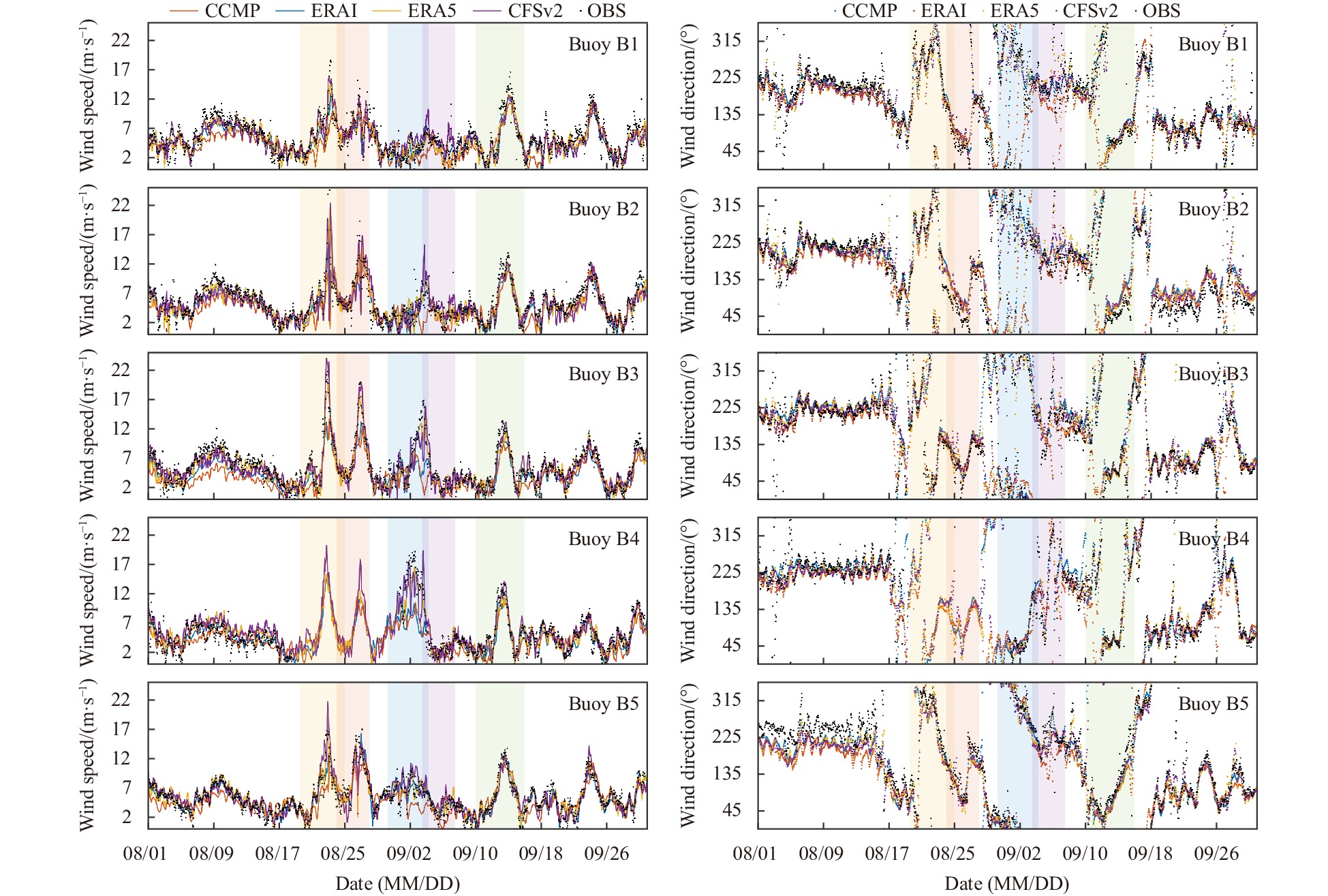
Figure 2. Time series of U10 (wind speed at 10 m height), wind direction between four wind data and corresponding buoy observations, with the time period from August 1 to September 30, 2017. The five periods of tropical cyclone (TC) occurrences are marked with a semi-transparent background color, from left to right: TC Hato, TC Pakhar, TC Mawar, TC Guchol, TC Doksuri. CCMP: Cross-Calibrated Multiplatform; ERAI: ECMWF Reanalysis-Interim; ERA5: ECMWF Reanalysis v5; CFSv2: NCEP Climate Forecast System Version 2; OBS: buoy observation.

Figure 3. Taylor diagram of wind speeds at 10 m height (U10) comparison at five buoys. The three rows from top to bottom are the entire period of this study (from August 1 to September 30, 2017), tropical cyclone (TC)-only period, and TC-free period, respectively. The Points A, B, C, D, O in the Taylor diagram represent CCMP, ERAI, ERA5, CFSv2, and buoy observations, respectively. CCMP: Cross-Calibrated Multiplatform; ERAI: ECMWF Reanalysis-Interim; ERA5: ECMWF Reanalysis v5; CFSv2: NCEP Climate Forecast System Version 2.

Figure 4. Scatter diagram of wind speeds at 10 m height (U10) obtained from four wind data and buoy observations between August 1 and September 30, 2017. The five columns from left to right represent five buoys. The x-axis represents U10 selected from the buoy observations, the y-axis represents U10 from the four wind products. The black lines represent for the perfect agreement between wind data and observations. The red lines and blue lines are fitted lines from different fitting formulas. CCMP: Cross-Calibrated Multiplatform; ERAI: ECMWF Reanalysis-Interim; ERA5: ECMWF Reanalysis v5; CFSv2: NCEP Climate Forecast System Version 2.

Figure 5. Magnitude of time-averaged wind speed in the study area. The four columns from left to right represent four wind data. The three rows from top to bottom represent the entire period, tropical cyclone (TC)-only period, and TC-free period. The black dots are the buoy positions. CCMP: Cross-Calibrated Multiplatform; ERAI: ECMWF Reanalysis-Interim; ERA5: ECMWF Reanalysis v5; CFSv2: NCEP Climate Forecast System Version 2.
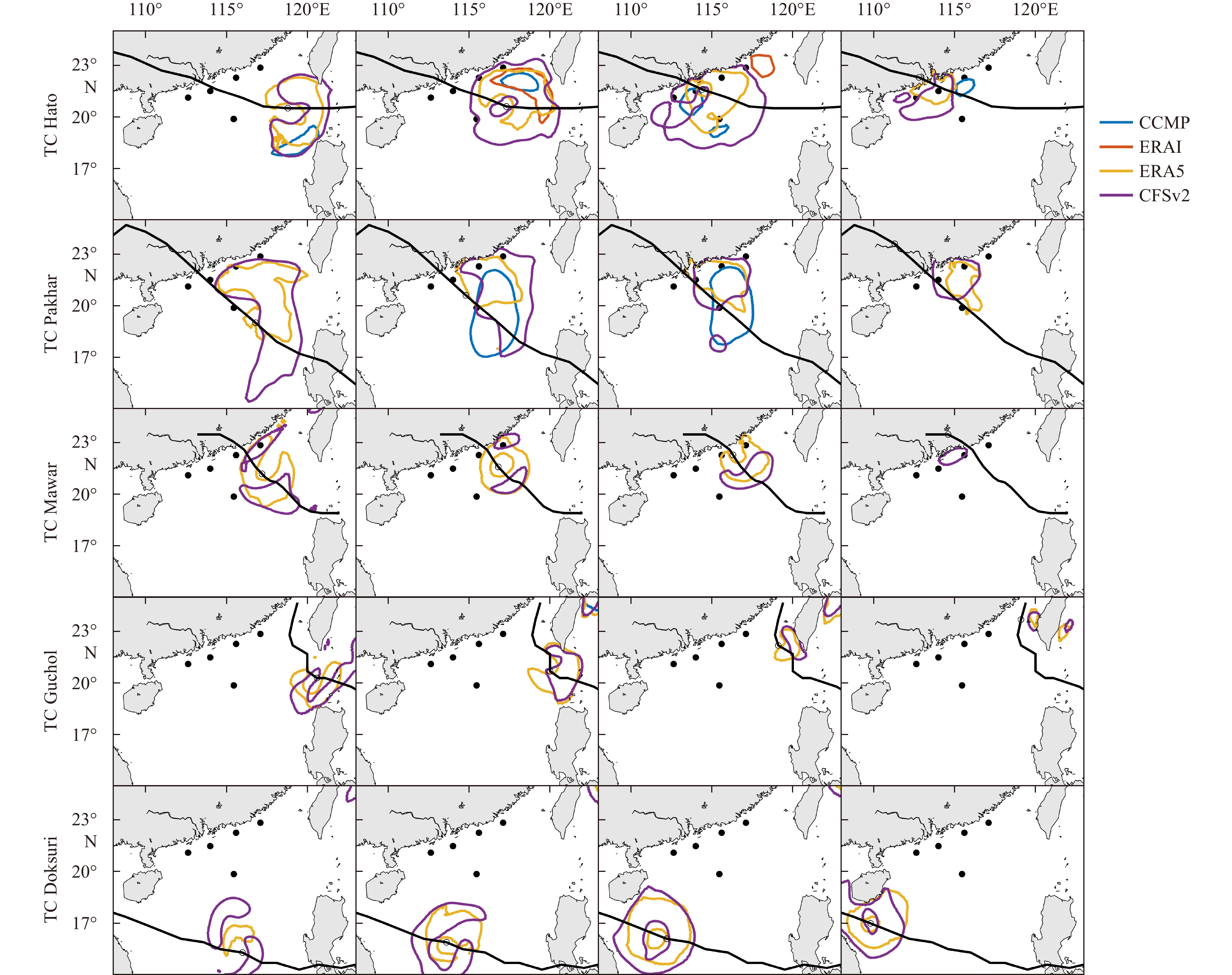
Figure 6. Contour distribution of the 99th percentile on wind speed during tropical cyclones (TCs). The five rows from top to bottom are five TC periods. The four columns are four snapshots during the TCs. The black lines are the TC tracks. The four colored contours represent four wind data. CCMP: Cross-Calibrated Multiplatform; ERAI: ECMWF Reanalysis-Interim; ERA5: ECMWF Reanalysis v5; CFSv2: NCEP Climate Forecast System Version 2.

Figure 7. Time series comparison of Hs and wave direction obtained from corresponding wave hindcast and buoy observations. The five periods of tropical cyclone occurrences are marked with a semi-transparent background color, from left to right: TC Hato, TC Pakhar, TC Mawar, TC Guchol, TC Doksuri. Hs: significant wave height; CCMP: Cross-Calibrated Multiplatform; ERAI: ECMWF Reanalysis-Interim; ERA5: ECMWF Reanalysis v5; CFSv2: NCEP Climate Forecast System Version 2; OBS: buoy observation.

Figure 8. Time series comparison of mean absolute wave period (Tm01) and peak period of variance density spectrum (Rtp) obtained from corresponding wave hindcast and buoy observations. The five periods of tropical cyclone occurrences are marked with a semi-transparent background color. Tm01: mean absolute wave period; CCMP: Cross-Calibrated Multiplatform; ERAI: ECMWF Reanalysis-Interim; ERA5: ECMWF Reanalysis v5; CFSv2: NCEP Climate Forecast System Version 2; OBS: buoy observation.

Figure 9. Taylor diagram of significant wave height comparison at five buoys. The three rows from top to bottom are the entire period, tropical cyclone (TC)-only period, and TC-period. The Points A, B, C, D, O in the Taylor diagram represent CCMP, ERAI, ERA5, CFSv2, and buoy observations, respectively. CCMP: Cross-Calibrated Multiplatform; ERAI: ECMWF Reanalysis-Interim; ERA5: ECMWF Reanalysis v5; CFSv2: NCEP Climate Forecast System Version 2.

Figure 10. Scatter plot of Hs obtained from wave hindcasts and buoy observations over the entire period. The five columns from left to right represent five buoys. The x-axis represents Hs selected from buoy observations, the y-axis represents Hs from the four wind products. The black lines represent perfect agreement between wind data and observations. The red and blue lines are fitted lines from different fitting formulas. Hs: significant wave height; CCMP: Cross-Calibrated Multiplatform; ERAI: ECMWF Reanalysis-Interim; ERA5: ECMWF Reanalysis v5; CFSv2: NCEP Climate Forecast System Version 2.

Figure 11. Magnitude of time-averaged Hs in the study area. The four columns from left to right represent four wind data. The three rows from top to bottom represent for entire period, tropical cyclone-only period, and tropical cyclone-free period. The black dots are the buoy positions. Hs: significant wave height; CCMP: Cross-Calibrated Multiplatform; ERAI: ECMWF Reanalysis-Interim; ERA5: ECMWF Reanalysis v5; CFSv2: NCEP Climate Forecast System Version 2.

Figure 12. Contour distribution of the 99th percentile of significant wave heights during tropical cyclone (TCs). The five rows from top to bottom are five TC periods. The four columns are four snapshots during the TCs. The black lines are the TC tracks. The four colored contours represent four wind data. CCMP: Cross-Calibrated Multiplatform; ERAI: ECMWF Reanalysis-Interim; ERA5: ECMWF Reanalysis v5; CFSv2: NCEP Climate Forecast System Version 2.

Figure 13. Waverose diagram of significant wave height (Hs) and wave direction obtained from experiments with different resolutions. The five rows from top to bottom correspond to the original results (Ori), spatial resolution of 0.5˚, spatial resolution of 1.0˚, temporal resolution of 3 h, and temporal resolution of 6 h, respectively. The five columns from left to right are at Buoys B1−B5. The three colors in each plot represent different ranges of Hs.

Figure 14. Contours represent the 99th percentile of significant wave height under different resolution experiments. The five rows from top to bottom are five tropical cyclone (TC) periods. The four columns are four snapshots during the TCs. The black lines are the TC tracks. CCMP: Cross-Calibrated Multiplatform; ERAI: ECMWF Reanalysis-Interim; ERA5: ECMWF Reanalysis v5; CFSv2: NCEP Climate Forecast System Version 2.
Table 1. Features of wind datasets
Data source Temporal coverage Temporal resolution/h Spatial resolution ERAI 1979−2019 3 0.25° ERA5 1979−2021 3 0.25° CFSv2 2011−present 1 0.125° CCMP 1987−present 6 0.25° Note: ERAI: ECMWF Reanalysis-Interim; ERA5: ECMWF Reanalysis v5; CFSv2: NCEP Climate Forecast System Version 2; CCMP: Cross-Calibrated Multiplatform.  下载: 导出CSV
Table 2. Features of buoys
Buoy Latitude Longitude Depth/m Number of Samples B1 21.12°N 112.63°E 50.43 1468 B2 21.50°N 114.00°E 54.02 1478 B3 22.28°N 115.60°E 49.17 1635 B4 22.87°N 117.10°E 40.60 1172 B5 19.87°N 115.46°E 1243.69 1472
下载: 导出CSV
Table 3. Average value (mean), maximum value of wind speed at 10 m height (U10) of the four wind data and corresponding hour when reaching the maximum value during each tropical cyclone period
Mean U10/(m·s−1) Maximum U10/(m·s−1) Occurrence of maximum U10/h Hato Pakhar Mawar Guchol Doksuri Hato Pakhar Mawar Guchol Doksuri Hato Pakhar Mawar Guchol Doksuri Buoy B1 6.67 7.20 3.38 3.26 6.25 18.60 15.20 7.40 11.10 16.60 92 64 113 33 104 CCMP 5.71 6.85 2.91 2.97 5.67 12.96 9.77 7.37 4.39 12.46 91 67 115 39 97 ERAI 4.69 7.30 2.29 1.60 5.70 10.05 9.97 4.71 2.97 11.67 97 64 31 42 109 ERA5 6.22 7.08 3.33 2.16 5.84 14.57 12.15 6.86 4.95 12.78 92 67 118 22 97 CFSv2 7.18 7.30 4.56 4.52 5.53 15.70 12.72 10.33 8.05 12.71 87 67 120 26 99 Buoy B2 7.41 8.11 4.09 2.94 5.54 43.40 19.30 11.10 10.60 13.90 87 69 79 39 96 CCMP 5.53 7.45 3.42 2.82 4.71 15.68 13.28 7.59 4.57 11.68 85 79 115 39 97 ERAI 4.92 7.92 2.80 1.66 5.00 12.09 11.59 5.19 3.43 10.96 97 79 43 39 97 ERA5 6.69 8.02 4.13 3.15 5.22 21.42 15.17 9.32 5.51 12.16 89 74 112 29 92 CFSv2 6.93 8.35 4.13 4.69 5.17 22.39 16.87 15.34 6.83 12.47 91 76 109 42 91 Buoy B3 6.94 8.22 7.25 2.74 5.26 21.80 20.00 16.90 5.40 13.40 83 71 107 43 80 CCMP 5.33 6.94 4.56 2.09 4.21 15.52 13.25 7.00 3.59 9.82 91 73 121 45 91 ERAI 5.16 6.81 4.16 1.23 3.98 13.91 12.25 7.65 2.12 9.45 91 76 85 45 82 ERA5 6.37 8.06 6.75 2.44 4.83 19.68 18.11 14.94 5.00 11.41 83 68 110 41 82 CFSv2 7.48 8.39 6.54 2.49 5.17 24.04 20.01 15.98 4.79 13.23 80 74 111 45 90 Buoy B4 NaN NaN 12.96 3.03 5.56 NaN NaN 19.20 5.60 13.80 NaN NaN 81 40 82 CCMP 5.54 5.74 7.30 2.45 4.56 15.29 11.31 11.13 4.80 11.32 79 73 43 45 85 ERAI 5.72 5.70 6.92 1.52 4.37 15.43 11.61 10.57 2.55 10.62 82 61 82 42 85 ERA5 5.80 6.14 10.46 3.07 5.06 15.32 13.11 16.58 6.50 11.61 78 67 80 41 80 CFSv2 6.89 6.65 10.78 2.74 5.75 20.22 17.97 19.33 6.18 14.15 80 70 105 45 85 Buoy B5 6.42 8.59 6.53 3.84 6.00 16.80 17.00 10.30 6.20 13.80 81 76 74 18 94 CCMP 6.10 8.60 6.78 4.11 5.48 13.83 16.30 8.81 5.13 11.56 91 73 25 21 97 ERAI 5.54 7.91 4.64 1.90 6.10 14.00 11.15 6.69 3.77 11.29 88 76 31 39 85 ERA5 6.60 8.50 7.07 4.52 5.70 16.38 14.52 10.04 7.16 12.47 82 58 72 40 90 CFSv2 7.35 8.36 7.71 4.99 5.53 21.72 14.59 11.20 7.58 12.92 83 73 69 18 87 Note: CCMP: Cross-Calibrated Multiplatform; ERAI: ECMWF Reanalysis-Interim; ERA5: ECMWF Reanalysis v5; CFSv2: NCEP Climate Forecast System Version 2. NaN indicates data unavailability.
下载: 导出CSV
Table 4. Statistical parameters for RMSE, r2, BIAS, SI and fitting coefficients (b and c) of wind speed at 10 m height (U10) based on four wind data and buoy observations during entire period, tropical cyclone (TC)-only period, and TC-free period
Entire period TC-only period TC-free period RMSE r2 BIAS SI b c RMSE r2 BIAS SI b c RMSE r2 BIAS SI b c Buoy B1 CCMP 0.49 0.88 0.68 0.09 0.68 0.83 0.48 0.88 0.62 0.09 0.71 0.84 0.50 0.88 0.71 0.09 0.64 0.83 ERAI 0.68 0.73 0.99 0.12 0.55 0.76 0.66 0.75 1.12 0.12 0.60 0.74 0.71 0.71 0.91 0.12 0.48 0.77 ERA5 0.49 0.87 0.46 0.09 0.76 0.88 0.46 0.89 0.39 0.08 0.78 0.89 0.53 0.85 0.50 0.08 0.75 0.88 CFSv2 0.55 0.83 0.19 0.10 0.71 0.91 0.52 0.85 −0.27 0.09 0.73 0.96 0.56 0.83 0.47 0.10 0.68 0.87 Buoy B2 CCMP 0.60 0.81 0.82 0.11 0.58 0.78 0.66 0.76 0.95 0.11 0.52 0.72 0.45 0.90 0.74 0.12 0.72 0.84 ERAI 0.74 0.67 0.97 0.13 0.47 0.73 0.77 0.64 1.27 0.13 0.43 0.65 0.67 0.75 0.79 0.15 0.59 0.80 ERA5 0.55 0.83 0.43 0.10 0.69 0.86 0.58 0.82 0.26 0.10 0.65 0.84 0.51 0.86 0.53 0.11 0.75 0.87 CFSv2 0.69 0.74 0.26 0.12 0.63 0.86 0.71 0.71 0.02 0.12 0.61 0.85 0.62 0.78 0.40 0.14 0.66 0.88 Buoy B3 CCMP 0.53 0.87 1.28 0.09 0.60 0.72 0.56 0.84 1.57 0.09 0.57 0.69 0.47 0.90 1.10 0.11 0.66 0.76 ERAI 0.65 0.76 1.61 0.12 0.52 0.66 0.65 0.76 1.89 0.10 0.53 0.65 0.68 0.73 1.44 0.13 0.47 0.67 ERA5 0.37 0.93 0.39 0.07 0.83 0.90 0.33 0.94 0.43 0.05 0.87 0.91 0.44 0.90 0.37 0.07 0.76 0.89 CFSv2 0.49 0.88 0.17 0.09 0.86 0.94 0.48 0.89 0.07 0.08 0.92 0.97 0.51 0.86 0.23 0.10 0.69 0.90 Buoy B4 CCMP 0.62 0.80 0.86 0.12 0.52 0.74 0.61 0.83 2.12 0.09 0.49 0.62 0.61 0.80 0.39 0.14 0.70 0.87 ERAI 0.65 0.78 1.09 0.13 0.48 0.69 0.61 0.82 2.36 0.09 0.48 0.59 0.71 0.71 0.62 0.14 0.54 0.80 ERA5 0.43 0.91 −0.08 0.08 0.74 0.93 0.32 0.96 0.59 0.05 0.79 0.87 0.64 0.77 −0.34 0.07 0.67 1.00 CFSv2 0.50 0.86 −0.48 0.10 0.76 0.99 0.45 0.89 0.15 0.06 0.80 0.91 0.65 0.77 −0.72 0.10 0.69 1.07 Buoy B5 CCMP 0.42 0.91 0.21 0.08 0.79 0.92 0.44 0.90 0.06 0.07 0.77 0.94 0.42 0.91 0.29 0.09 0.76 0.91 ERAI 0.64 0.76 0.57 0.12 0.59 0.83 0.64 0.77 0.92 0.10 0.61 0.80 0.68 0.73 0.37 0.13 0.56 0.86 ERA5 0.42 0.91 −0.18 0.08 0.82 0.99 0.41 0.91 −0.21 0.06 0.80 0.98 0.47 0.88 −0.17 0.08 0.80 1.00 CFSv2 0.54 0.85 −0.20 0.10 0.85 1.00 0.56 0.84 −0.52 0.09 0.84 1.02 0.54 0.85 −0.01 0.11 0.79 0.97 Note: RMSE: root mean square error; r2: correlation coefficient; SI: scatter index; CCMP: Cross-Calibrated Multiplatform; ERAI: ECMWF Reanalysis-Interim; ERA5: ECMWF Reanalysis v5; CFSv2: NCEP Climate Forecast System Version 2.
下载: 导出CSV
Table 5. The average value of significant wave height (Hs) (mean Hs), maximum value of Hs from wave hindcasts, and the corresponding time when reaching the maximum values during tropical cyclones for buoy observations and four wind data
Mean Hs/m Maximum Hs/m Occurence of maximum Hs/h Hato Pakhar Mawar Guchol Doksuri Hato Pakhar Mawar Guchol Doksuri Hato Pakhar Mawar Guchol Doksuri Buoy B1 1.05 1.60 0.70 0.60 1.39 3.20 3.10 1.00 0.80 3.50 94 70 60 1 113 CCMP 0.92 1.22 0.77 0.67 1.31 2.32 1.95 0.97 0.79 2.87 93 91 117 1 100 ERAI 0.84 1.21 0.74 0.61 1.27 1.67 1.88 0.87 0.75 2.54 97 68 75 1 110 ERA5 1.07 1.35 0.90 0.72 1.43 2.72 2.58 1.22 0.78 3.30 90 70 71 1 105 CFSv2 1.27 1.47 0.99 0.86 1.49 3.74 2.80 1.56 1.03 3.54 88 71 121 27 102 Buoy B2 1.44 1.96 1.03 0.64 1.36 8.50 5.40 1.80 0.90 3.00 87 69 82 3 99 CCMP 1.01 1.46 0.89 0.65 1.23 2.98 2.93 1.12 0.74 2.61 86 83 59 1 98 ERAI 0.96 1.36 0.86 0.60 1.22 2.34 2.29 1.05 0.72 2.34 86 65 70 1 87 ERA5 1.27 1.62 1.09 0.68 1.39 4.21 3.49 1.63 0.74 2.86 84 68 74 1 103 CFSv2 1.43 1.78 1.19 0.81 1.47 4.97 4.04 2.04 0.95 3.16 83 68 109 42 102 Buoy B3 1.47 2.13 1.85 0.61 1.22 6.10 6.00 2.90 0.80 2.60 82 70 106 36 121 CCMP 1.19 1.65 1.07 0.70 1.16 3.47 3.55 1.37 0.74 2.34 81 79 70 1 88 ERAI 1.27 1.42 1.07 0.65 1.15 3.36 2.61 1.43 0.71 2.31 82 64 87 1 84 ERA5 1.51 1.95 1.61 0.75 1.33 5.00 5.00 2.71 0.84 2.65 83 69 110 42 82 CFSv2 1.79 2.13 1.70 0.76 1.47 6.66 5.70 2.94 0.84 3.07 81 68 113 42 91 Buoy B4 NaN NaN 2.86 0.65 1.25 NaN NaN 3.90 1.10 2.90 NaN NaN 99 36 128 CCMP 1.24 1.38 1.25 0.64 1.02 3.64 2.68 1.77 0.67 2.16 80 80 44 24 86 ERAI 1.29 1.20 1.15 0.56 1.02 3.65 2.32 1.55 0.58 2.08 81 64 83 29 83 ERA5 1.38 1.53 2.04 0.71 1.16 3.82 3.09 3.14 0.84 2.28 80 67 82 42 81 CFSv2 1.62 1.78 2.14 0.70 1.33 5.07 4.70 4.29 0.79 2.75 80 71 106 45 88 Buoy B5 1.60 2.19 1.80 0.81 1.47 4.40 4.20 2.90 0.90 3.50 92 62 82 8 93 CCMP 1.21 1.83 1.34 0.84 1.40 2.77 3.76 1.72 0.90 2.81 91 75 52 1 84 ERAI 1.05 1.35 1.13 0.75 1.44 2.60 2.03 1.40 0.88 2.87 91 78 55 1 82 ERA5 1.48 1.84 1.54 0.93 1.61 3.54 3.31 2.27 1.01 3.23 84 59 73 18 95 CFSv2 1.73 1.94 1.69 0.94 1.69 4.88 3.42 2.47 1.10 3.71 86 59 71 19 96 Note: CCMP: Cross-Calibrated Multiplatform; ERAI: ECMWF Reanalysis-Interim; ERA5: ECMWF Reanalysis v5; CFSv2: NCEP Climate Forecast System Version 2. NaN indicates data unavailability.
下载: 导出CSV
Table 6. Statistical parameters of RMSE, r2, BIAS, SI and fitting coefficients (b and c) for Hs obtained from four wind data and buoy observations during entire period, tropical cyclone (TC)-only period, and TC-free period
Entire period TC-only period TC-free period RMSE r2 BIAS SI b c RMSE r2 BIAS SI b c RMSE r2 BIAS SI b c Buoy B1 CCMP 0.43 0.92 0.09 0.45 0.69 0.85 0.39 0.94 0.08 0.35 0.72 0.86 0.52 0.89 0.09 0.44 0.57 0.83 ERAI 0.55 0.86 0.12 0.58 0.57 0.79 0.48 0.91 0.13 0.44 0.61 0.80 0.70 0.73 0.12 0.54 0.44 0.78 ERA5 0.39 0.92 −0.03 0.41 0.77 0.96 0.36 0.93 −0.04 0.33 0.80 0.96 0.46 0.90 −0.03 0.41 0.66 0.95 CFSv2 0.43 0.90 −0.07 0.45 0.86 1.02 0.38 0.93 −0.16 0.35 0.91 1.07 0.48 0.88 −0.03 0.43 0.68 0.96 Buoy B2 CCMP 0.53 0.89 0.17 0.50 0.55 0.74 0.55 0.89 0.27 0.40 0.53 0.70 0.54 0.86 0.12 0.60 0.58 0.81 ERAI 0.63 0.82 0.19 0.60 0.46 0.69 0.63 0.86 0.32 0.46 0.43 0.64 0.72 0.69 0.13 0.69 0.49 0.78 ERA5 0.43 0.92 0.04 0.41 0.68 0.86 0.44 0.92 0.09 0.32 0.67 0.84 0.51 0.88 0.03 0.48 0.63 0.90 CFSv2 0.45 0.89 0.00 0.43 0.77 0.92 0.45 0.89 −0.04 0.33 0.76 0.93 0.53 0.85 0.01 0.49 0.68 0.91 Buoy B3 CCMP 0.53 0.88 0.17 0.48 0.57 0.75 0.56 0.86 0.32 0.36 0.55 0.70 0.52 0.88 0.10 0.61 0.61 0.86 ERAI 0.60 0.84 0.20 0.55 0.49 0.70 0.60 0.86 0.36 0.39 0.48 0.66 0.77 0.64 0.13 0.65 0.42 0.79 ERA5 0.30 0.96 −0.02 0.27 0.82 0.95 0.27 0.97 0.02 0.18 0.84 0.93 0.48 0.89 −0.04 0.30 0.67 0.98 CFSv2 0.35 0.94 −0.08 0.32 0.98 1.04 0.35 0.94 −0.15 0.23 1.01 1.06 0.47 0.88 −0.05 0.39 0.72 0.99 Buoy B4 CCMP 0.66 0.82 0.19 0.67 0.40 0.67 0.73 0.75 0.55 0.47 0.34 0.54 0.46 0.92 0.11 0.84 0.62 0.87 ERAI 0.71 0.78 0.24 0.72 0.34 0.62 0.73 0.76 0.59 0.47 0.32 0.52 0.72 0.71 0.16 0.85 0.40 0.78 ERA5 0.34 0.97 0.01 0.35 0.71 0.90 0.31 0.98 0.17 0.20 0.73 0.84 0.45 0.92 −0.03 0.36 0.65 0.99 CFSv2 0.43 0.91 −0.04 0.44 0.74 0.94 0.49 0.87 0.06 0.32 0.73 0.89 0.43 0.92 −0.06 0.57 0.68 1.02 Buoy B5 CCMP 0.47 0.90 0.13 0.39 0.66 0.83 0.51 0.88 0.27 0.31 0.62 0.78 0.47 0.89 0.06 0.50 0.73 0.91 ERAI 0.64 0.80 0.21 0.53 0.46 0.72 0.66 0.79 0.45 0.40 0.43 0.66 0.67 0.75 0.10 0.66 0.54 0.84 ERA5 0.37 0.94 −0.01 0.31 0.75 0.93 0.39 0.93 0.11 0.24 0.73 0.89 0.42 0.91 −0.06 0.39 0.82 1.02 CFSv2 0.35 0.94 −0.05 0.29 0.91 1.00 0.35 0.94 −0.04 0.21 0.90 1.00 0.48 0.88 −0.05 0.35 0.85 1.01 Note: Hs: significant wave height; RMSE: root mean square error; r2: correlation coefficient; SI: scatter index; CCMP: Cross-Calibrated Multiplatform; ERAI: ECMWF Reanalysis-Interim; ERA5: ECMWF Reanalysis v5; CFSv2: NCEP Climate Forecast System Version 2.
下载: 导出CSV
-
Atlas R, Hoffman R N, Bloom S C, et al. 1996. A multiyear global surface wind velocity dataset using SSM/I wind observations. Bulletin of the American Meteorological Society, 77(5): 869–882. doi: 10.1175/1520-0477(1996)077<0869:AMGSWV>2.0.CO;2 Atlas R, Hoffman R N, Ardizzone J, et al. 2011. A cross-calibrated, multiplatform ocean surface wind velocity product for meteorological and oceanographic applications. Bulletin of the American Meteorological Society, 92(2): 157–174. doi: 10.1175/2010BAMS2946.1 Battjes J A, Janssen J P F M. 1978. Energy loss and set-up due to breaking of random waves. In: Proceedings of the 16th International Conference on Coastal Engineering. Hamburg, Germany: American Society of Civil Engineers, 569–587 Becerra D, Quezada M, Díaz H. 2022. A deep water and nearshore wave height calibration of the ECOWAVES hindcasting database. Latin American Journal of Aquatic Research, 50(4): 573–595. doi: 10.3856/vol50-issue4-fulltext-2811 Booij N, Ris R C, Holthuijsen L H. 1999. A third-generation wave model for coastal regions: 1. Model description and validation. Journal of Geophysical Research: Oceans, 104(C4): 7649–7666. doi: 10.1029/98JC02622 Bourassa M A, Legler D M, O’Brien J J, et al. 2003. SeaWinds validation with research vessels. Journal of Geophysical Research: Oceans, 108(C2): 3019 Carvalho D, Rocha A, Gómez-Gesteira M, et al. 2014. Comparison of reanalyzed, analyzed, satellite-retrieved and NWP modelled winds with buoy data along the Iberian Peninsula coast. Remote Sensing of Environment, 152: 480–492. doi: 10.1016/j.rse.2014.07.017 Cavaleri L, Rizzoli P M. 1981. Wind wave prediction in shallow water: Theory and applications. Journal of Geophysical Research: Oceans, 86(C11): 10961–10973. doi: 10.1029/JC086iC11p10961 Chalikov D. 2018. Numerical modeling of surface wave development under the action of wind. Ocean Science, 14(3): 453–470. doi: 10.5194/os-14-453-2018 Chauvin F, Douville H, Ribes A. 2017. Atlantic tropical cyclones water budget in observations and CNRM-CM5 model. Climate Dynamics, 49(11): 4009–4021 Chelton D B, Freilich M H. 2005. Scatterometer-based assessment of 10-m wind analyses from the operational ECMWF and NCEP numerical weather prediction models. Monthly Weather Review, 133(2): 409–429. doi: 10.1175/MWR-2861.1 Chen Weibo, Chen Hongey, Hsiao Shihchun, et al. 2019. Wind forcing effect on hindcasting of typhoon-driven extreme waves. Ocean Engineering, 188: 106260. doi: 10.1016/j.oceaneng.2019.106260 Dee D P, Uppala S M, Simmons A J, et al. 2011. The ERA-Interim reanalysis: Configuration and performance of the data assimilation system. Quarterly Journal of the Royal Meteorological Society, 137(656): 553–597. doi: 10.1002/qj.828 Gualtieri G. 2021. Reliability of ERA5 reanalysis data for wind resource assessment: A comparison against tall towers. Energies, 14(14): 4169. doi: 10.3390/en14144169 Hasselmann K, Barnett T, Bouws E, et al. 1973. Measurements of wind-wave growth and swell decay during the Joint North Sea Wave Project (JONSWAP). In: Ergänzungsheft zur Deutschen Hydrographischen Zeitschrift. Hamburg: Deutches Hydrographisches Institut, 8: 1–95 Hasselmann S, Hasselmann K, Allender J H, et al. 1985. Computations and parameterizations of the nonlinear energy transfer in a gravity-wave spectrum. Part II: Parameterizations of the nonlinear energy transfer for application in wave models. Journal of Physical Oceanography, 15(11): 1378–1391. doi: 10.1175/1520-0485(1985)015<1378:CAPOTN>2.0.CO;2 Hawkins S, Eager D, Harrison G P. 2011. Characterising the reliability of production from future British offshore wind fleets. In: IET Conference on Renewable Power Generation (RPG 2011). Edinburgh: IET Hersbach H, Bell B, Berrisford P, et al. 2020. The ERA5 global reanalysis. Quarterly Journal of the Royal Meteorological Society, 146(730): 1999–2049. doi: 10.1002/qj.3803 Hoffman R N, Leidner S M, Henderson J M, et al. 2003. A two-dimensional variational analysis method for NSCAT ambiguity removal: Methodology, sensitivity, and tuning. Journal of Atmospheric and Oceanic Technology, 20(5): 585–605. doi: 10.1175/1520-0426(2003)20<585:ATDVAM>2.0.CO;2 Janssen P A E M. 1989. Wave-induced stress and the drag of air flow over sea waves. Journal of Physical Oceanography, 19(6): 745–754. doi: 10.1175/1520-0485(1989)019<0745:WISATD>2.0.CO;2 Jun K C, Jeong W M, Choi J Y, et al. 2015. Simulation of the extreme waves generated by typhoon Bolaven (1215) in the East China Sea and Yellow Sea. Acta Oceanologica Sinica, 34(12): 19–28. doi: 10.1007/s13131-015-0779-4 Kanwal A, Tahir Z R, Asim M, et al. 2022. Evaluation of Reanalysis and Analysis Datasets Against Measured Wind Data for Wind Resource Assessment. Bonn, Germany: World Wind Energy Association Kara A B, Wallcraft A J, Bourassa M A. 2008. Air-sea stability effects on the 10 m winds over the global ocean: Evaluations of air-sea flux algorithms. Journal of Geophysical Research: Oceans, 113(C4): C04009 Komen G J, Hasselmann K, Hasselmann K. 1984. On the existence of a fully developed wind-sea spectrum. Journal of Physical Oceanography, 14(8): 1271–1285. doi: 10.1175/1520-0485(1984)014<1271:OTEOAF>2.0.CO;2 Lavrenov I V. 2003. Wind-Waves in Oceans: Dynamics and Numerical Simulations. Berlin, Heidelberg: Springer Liu W Timothy, Tang Wenqing. 1996. Equivalent Neutral Wind. Washington, DC: National Aeronautics and Space Administration Mears C A, Smith D K, Wentz F. 2001. Comparison of Special Sensor Microwave Imager and buoy-measured wind speeds from 1987 to 1997. Journal of Geophysical Research, 106: 11719–11729. doi: 10.1029/1999JC000097 Monin A S, Obhukov A. 1954. Osnovnye zakonomernosti turbulentnogo peremeshivanija v prizemnon sloe atmosfery (Basic laws of turbulent mixing in the atmosphere near the ground). Trudy Geofizicheskogo Instituta, Akademiya Nauk SSSR, 24: 163–187 Morim J, Erikson L H, Hemer M, et al. 2022. A global ensemble of ocean wave climate statistics from contemporary wave reanalysis and hindcasts. Scientific Data, 9: 358. doi: 10.1038/s41597-022-01459-3 Peixoto J P, Oort A H. 1992. Physics of Climate. New York: American Institute of Physics Qiao Wenli, Song Jinbao, He Hailun, et al. 2019. Application of different wind field models and wave boundary layer model to typhoon waves numerical simulation in WAVEWATCH III model. Tellus A: Dynamic Meteorology and Oceanography, 71(1): 1657552. doi: 10.1080/16000870.2019.1657552 Rapizo H, Liu Qingxiang, Babanin A V. 2022. Performance of the observation-based source terms in a high-resolution wave hindcast for the North Sea. In: Proceedings of the 41st International Conference on Ocean, Offshore and Arctic Engineering: Volume 2: Structures, Safety, and Reliability. Hamburg, Germany: ASME Ruti P M, Marullo S, D’Ortenzio F, et al. 2008. Comparison of analyzed and measured wind speeds in the perspective of oceanic simulations over the Mediterranean basin: Analyses, QuikSCAT and buoy data. Journal of Marine Systems, 70(1–2): 33–48 Saha S, Moorthi S, Wu Xingren, et al. 2014. The NCEP Climate Forecast System version 2. Journal of Climate, 27(6): 2185–2208. doi: 10.1175/JCLI-D-12-00823.1 Snyder R L, Dobson F W, Elliott J A, et al. 1981. Array measurements of atmospheric pressure fluctuations above surface gravity waves. Journal of Fluid Mechanics, 102: 1–59. doi: 10.1017/S0022112081002528 Stopa J E. 2018. Wind forcing calibration and wave hindcast comparison using multiple reanalysis and merged satellite wind datasets. Ocean Modelling, 127: 55–69. doi: 10.1016/j.ocemod.2018.04.008 Taylor K E. 2005. Taylor diagram primer. https://pcmdi.llnl.gov/staff/taylor/CV/Taylor_diagram_primer.pdf[2005-01-23/2023-05-28] Van Vledder G P, Akpınar A. 2015. Wave model predictions in the Black Sea: Sensitivity to wind fields. Applied Ocean Research, 53: 161–178. doi: 10.1016/j.apor.2015.08.006 Wang Guo-sen, Wang Xidong, Wang Hui, et al. 2020. Evaluation on monthly sea surface wind speed of four reanalysis data sets over the China seas after 1988. Acta Oceanologica Sinica, 39(1): 83–90. doi: 10.1007/s13131-019-1525-0 Weintrit A. 2009. Marine Navigation and Safety of Sea Transportation (1st ed. ). London: CRC Press Wu Wenfang, Li Pieliang, Zhai Fanggou, et al. 2020. Evaluation of different wind resources in simulating wave height for the Bohai, Yellow, and East China Seas (BYES) with SWAN model. Continental Shelf Research, 207: 104217. doi: 10.1016/j.csr.2020.104217 Xie Shangping, Chang Chueh-hsin, Xie Qiang, et al. 2007. Intraseasonal variability in the summer South China Sea: Wind jet, cold filament, and recirculations. Journal of Geophysical Research: Oceans, 112(C10): C10008. doi: 10.1029/2007JC004238 -


 DownLoad:


 点击查看大图
计量
- 文章访问数: 776
- HTML全文浏览量: 346
- PDF下载量: 55
- 被引次数: 0

