

Rapid environmental assessment in the South China Sea: Improved inversion of sound speed profile using remote sensing data
-
Abstract: Complex perturbations in the profile and the sparsity of samples often limit the validity of rapid environmental assessment (REA) in the South China Sea (SCS). In this paper, the remote sensing data were used to estimate sound speed profile (SSP) with the self-organizing map (SOM) method in the SCS. First, the consistency of the empirical orthogonal functions was examined by using k-means clustering. The clustering results indicated that SSPs in the SCS have a similar perturbation nature, which means the inverted grid could be expanded to the entire SCS to deal with the problem of sparsity of the samples without statistical improbability. Second, a machine learning method was proposed that took advantage of the topological structure of SOM to significantly improve their accuracy. Validation revealed promising results, with a mean reconstruction error of 1.26 m/s, which is 1.16 m/s smaller than the traditional single empirical orthogonal function regression (sEOF-r) method. By violating the constraints of linear inversion, the topological structure of the SOM method showed a smaller error and better robustness in the SSP estimation. The improvements to enhance the accuracy and robustness of REA in the SCS were offered. These results suggested a potential utilization of REA in the SCS based on satellite data and provided a new approach for SSP estimation derived from sea surface data.
-
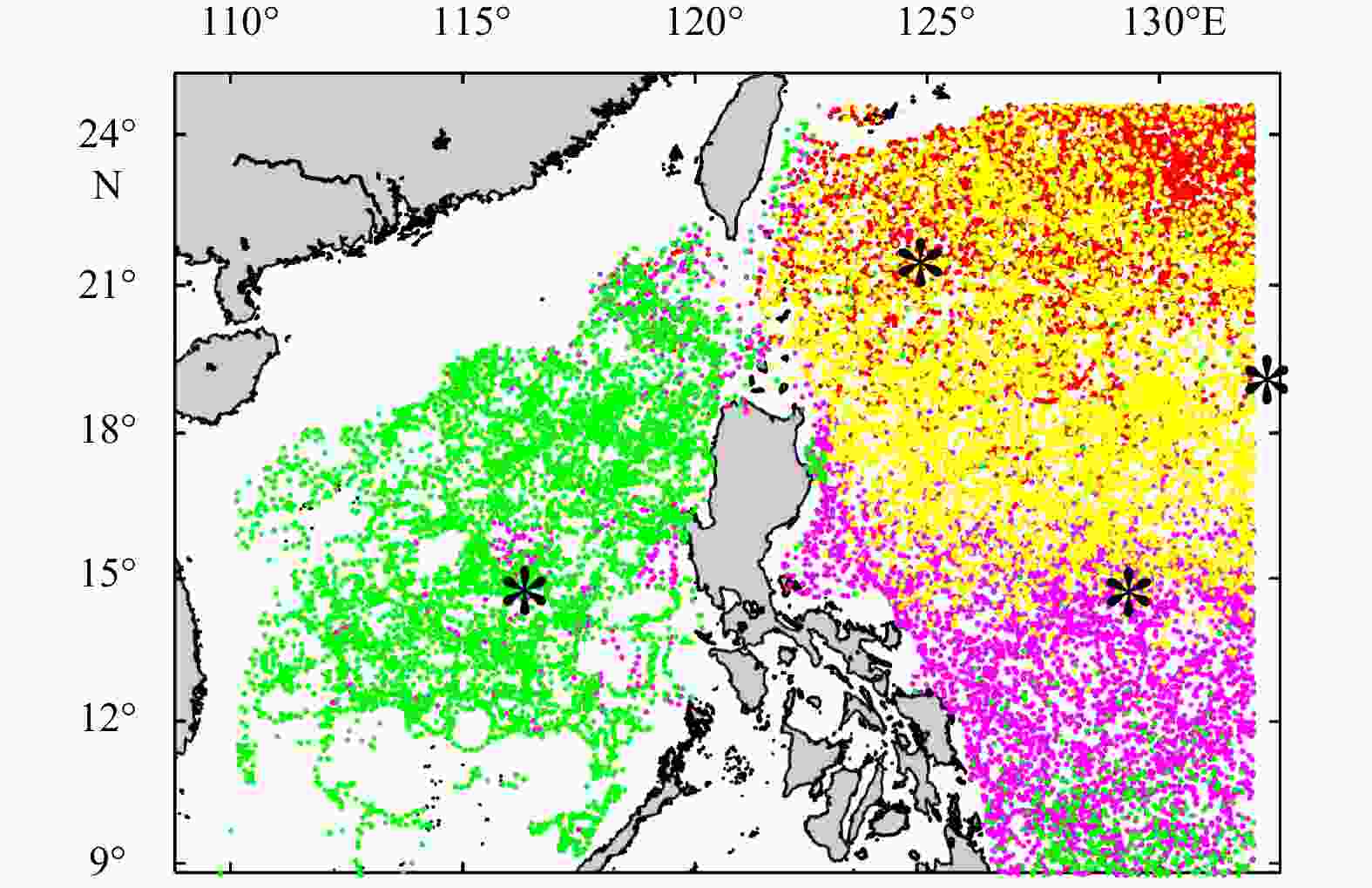
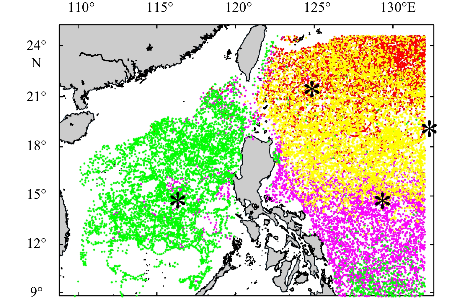
Figure 2. Distribution of clustered samples when five-order empirical orthogonal function coefficients were clustered into four classes. The class centers are marked by asterisks.
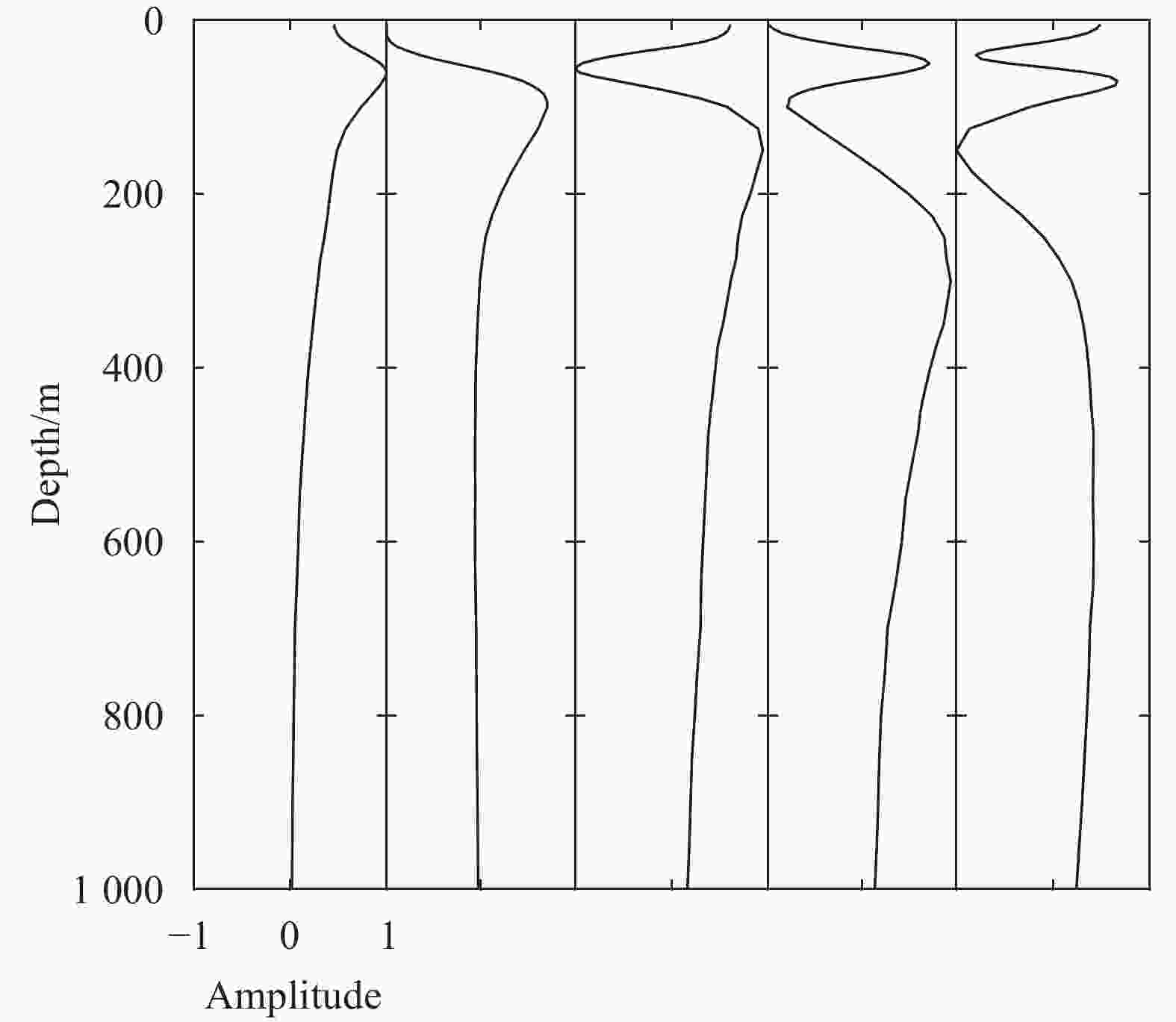
Figure 3. First five orders of the empirical orthogonal function. From left to right are, in order, the first to the fifth order.

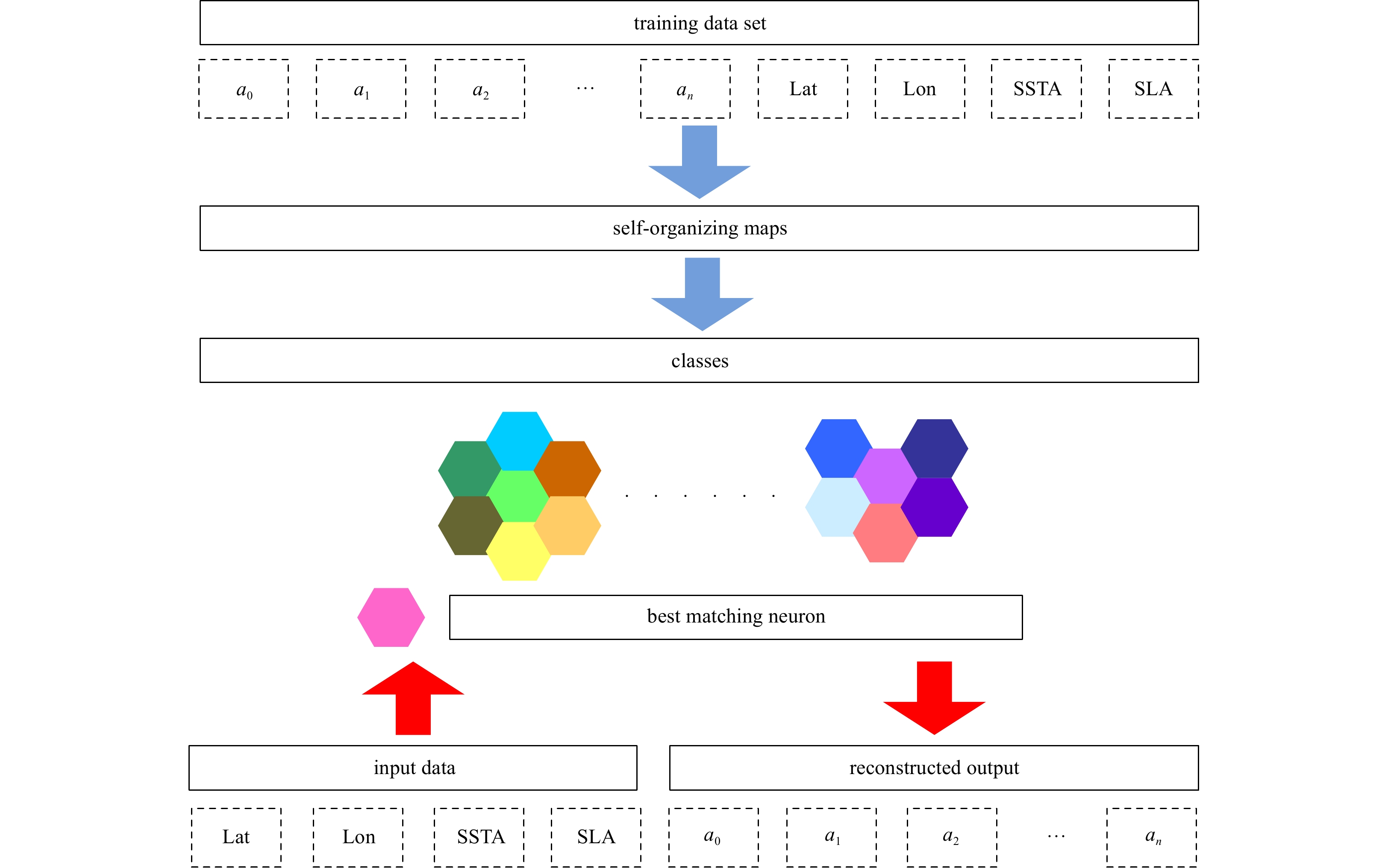
Figure 4. Schematics of the training of the map (blue arrows) and reconstruction of the sound speed profile (red arrows) using self-organizing map-based inversion. Lat: latitude; Lon: longitude; SSTA: sea surface temperature anomaly; SLA: sea level anomaly.
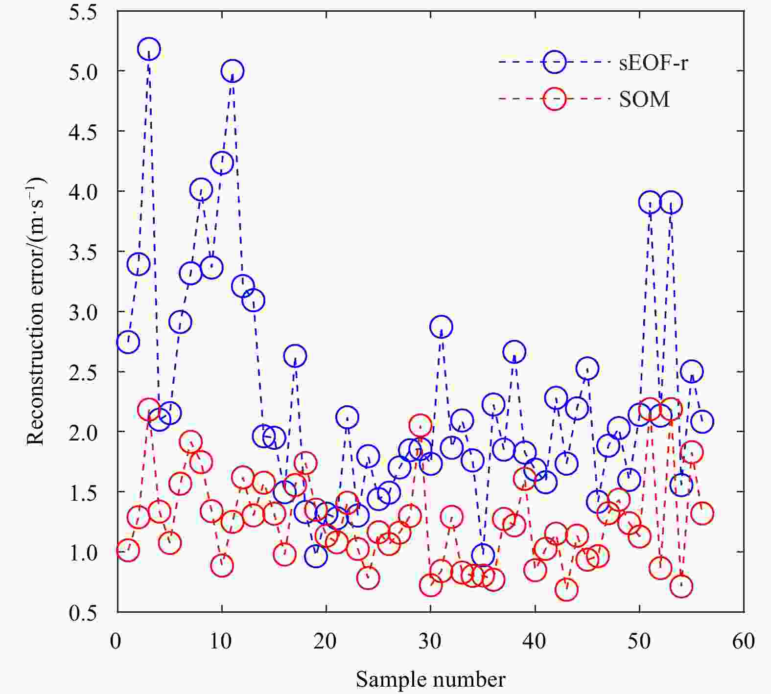
Figure 5. Errors of reconstruction for different sample numbers. EOF: empirical orthogonal function; SOM: self-organizing map.
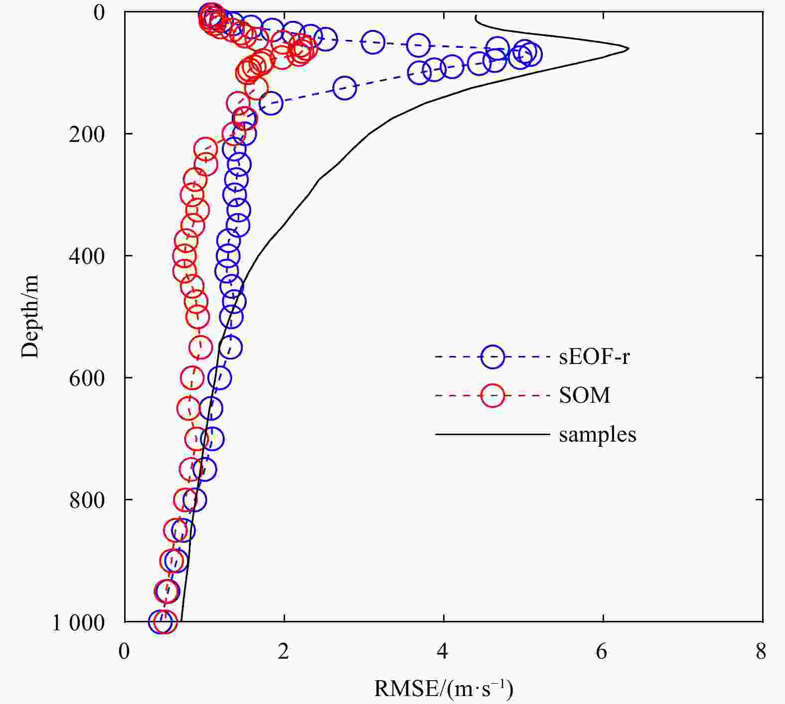
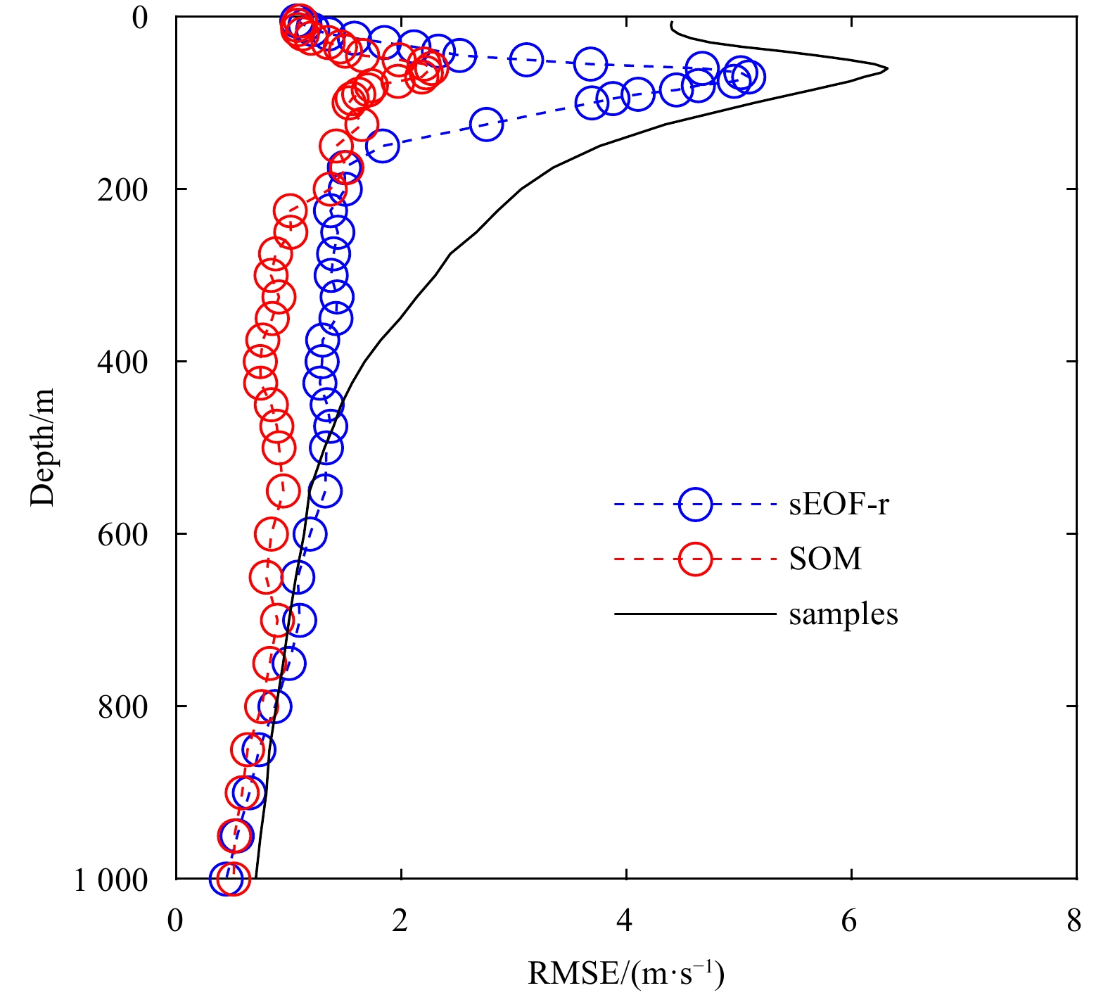
Figure 6. Reconstruction errors at different depths. EOF: empirical orthogonal function; SOM: self-organizing map.
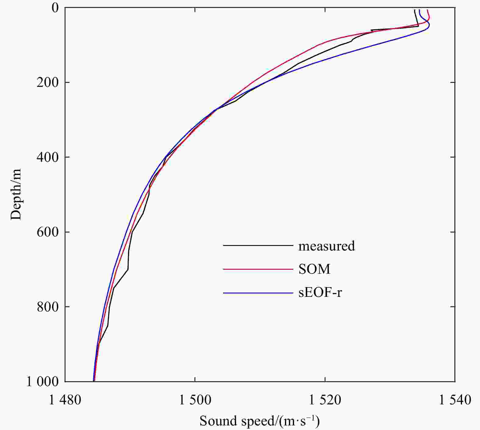
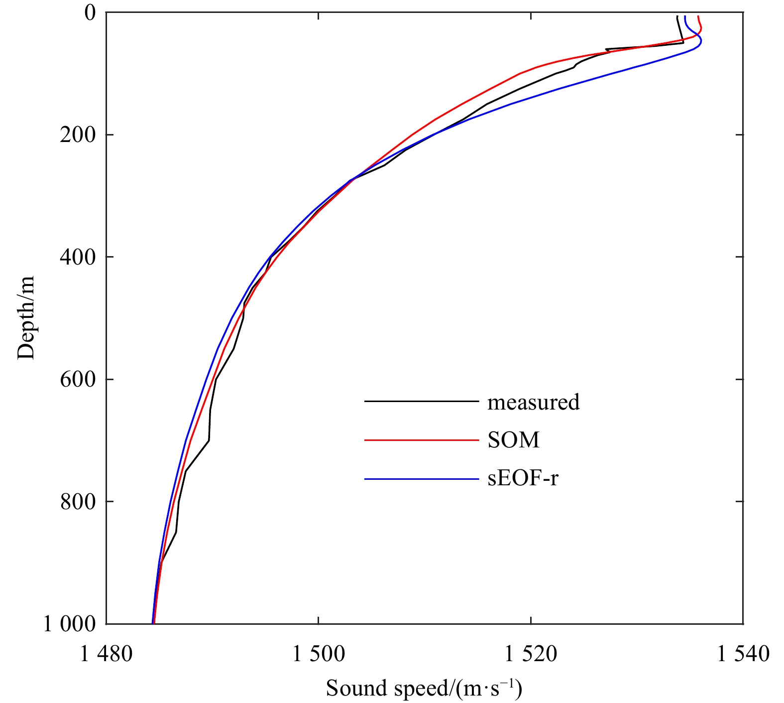
Figure 7. An example of sound speed profile reconstruction. The sample used had the largest error in self-organizing map (SOM) reconstruction. EOF: empirical orthogonal function.
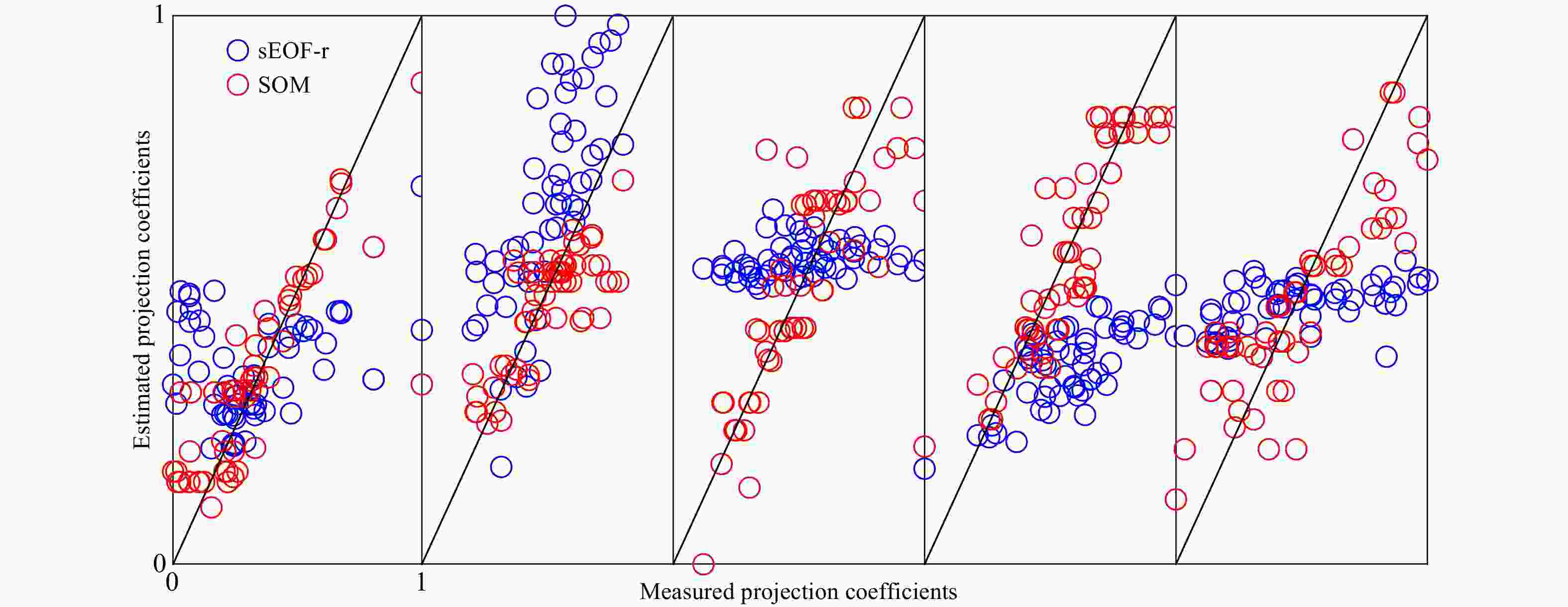
Figure 8. Results of inversion of the normalized projection coefficients of the first five orders. The straight line indicates perfect inversion. From left to right are, in order, the first to the fifth order. EOF: empirical orthogonal function; SOM: self-organizing map.
Table 1. Properties of reconstruction of different orders of the empirical orthogonal function (EOF)
EOF1 EOF2 EOF3 EOF4 EOF5 Variance contribution/% 74.0 13.7 4.7 2.9 1.4 Cumulative variance contribution/% 74.0 87.7 92.4 95.3 96.7 Reconstruction error/(m·s−1) 2.00 1.38 1.09 0.85 0.72  下载: 导出CSV
-
[1] Bao Senliang, Zhang Ren, Wang Huizan, et al. 2019. Salinity profile estimation in the Pacific Ocean from satellite surface salinity observations. Journal of Atmospheric and Oceanic Technology, 36(1): 53–68. doi: 10.1175/JTECH-D-17-0226.1 [2] Bianco M J, Gerstoft P. 2017. Dictionary learning of sound speed profiles. The Journal of the Acoustical Society of America, 141(3): 1749–1758. doi: 10.1121/1.4977926 [3] Carnes M R, Mitchell J L, de Witt P W. 1990. Synthetic temperature profiles derived from Geosat altimetry: Comparison with air-dropped expendable bathythermograph profiles. Journal of Geophysical Research, 95(C10): 17979–17992. doi: 10.1029/JC095iC10p17979 [4] Carnes M R, Teague W J, Mitchell J L. 1994. Inference of subsurface thermohaline structure from fields measurable by satellite. Journal of Atmospheric and Oceanic Technology, 11(2): 551–566. doi: 10.1175/1520-0426(1994)011<0551:IOSTSF>2.0.CO;2 [5] Chapman C, Charantonis A A. 2017. Reconstruction of subsurface velocities from satellite observations using iterative self-organizing maps. IEEE Geoscience and Remote Sensing Letters, 14(5): 617–620. doi: 10.1109/LGRS.2017.2665603 [6] Charantonis A A, Testor P, Mortier l, et al. 2015. Completion of a sparse GLIDER database using multi-iterative Self-Organizing Maps (ITCOMP SOM). Procedia Computer Science, 51: 2198–2206. doi: 10.1016/j.procs.2015.05.496 [7] Chen Cheng, Ma Yuanliang, Liu Ying. 2018. Reconstructing sound speed profiles worldwide with sea surface data. Applied Ocean Research, 77: 26–33. doi: 10.1016/j.apor.2018.05.002 [8] Del Grosso V A. 1974. New equation for the speed of sound in natural waters (with comparisons to other equations). The Journal of the Acoustical Society of America, 56(4): 1084–1091. doi: 10.1121/1.1903388 [9] Fox D N, Teague W J, Barron C N, et al. 2002. The modular ocean data assimilation system (MODAS). Journal of Atmospheric and Oceanic Technology, 19(2): 240–252. doi: 10.1175/1520-0426(2002)019<0240:TMODAS>2.0.CO;2 [10] Frederick C, Villar S, Michalopoulou Z H. 2020. Seabed classification using physics-based modeling and machine learning. The Journal of the Acoustical Society of America, 148(2): 859–872. doi: 10.1121/10.0001728 [11] Hjelmervik K T, Hjelmervik K. 2013. Estimating temperature and salinity profiles using empirical orthogonal functions and clustering on historical measurements. Ocean Dynamics, 63(7): 809–821. doi: 10.1007/s10236-013-0623-3 [12] Hjelmervik K, Hjelmervik K T. 2014. Time-calibrated estimates of oceanographic profiles using empirical orthogonal functions and clustering. Ocean Dynamics, 64(5): 655–665. doi: 10.1007/s10236-014-0704-y [13] Jain S, Ali M M. 2006. Estimation of sound speed profiles using artificial neural networks. IEEE Geoscience and Remote Sensing Letters, 3(4): 467–470. doi: 10.1109/LGRS.2006.876221 [14] LeBlanc L R, Middleton F H. 1980. An underwater acoustic sound velocity data model. The Journal of the Acoustical Society of America, 67(6): 2055–2062. doi: 10.1121/1.384448 [15] Li Zhaoqin, Liu Zenghong, Lu Shaolei. 2020. Global Argo data fast receiving and post-quality-control system. IOP Conference Series: Earth and Environmental Science, 502: 012012. doi: 10.1088/1755-1315/502/1/012012 [16] Meijers A J S, Bindoff N L, Rintoul S R. 2011. Estimating the four-dimensional structure of the Southern Ocean using satellite altimetry. Journal of Atmospheric and Oceanic Technology, 28(4): 548–568. doi: 10.1175/2010JTECHO790.1 [17] Rahaman H, Behringer B W, Penny S G, et al. 2016. Impact of an upgraded model in the NCEP Global Ocean Data Assimilation System: The tropical Indian Ocean. Journal of Geophysical Research: Oceans, 121(11): 8039–8062. doi: 10.1002/2016JC012056 [18] Su Hua, Yang Xin, Lu Wenfang, et al. 2019. Estimating subsurface thermohaline structure of the global ocean using surface remote sensing observations. Remote Sensing, 11(13): 1598. doi: 10.3390/rs11131598 -


 点击查看大图
计量
- 文章访问数: 293
- HTML全文浏览量: 82
- PDF下载量: 24
- 被引次数: 0

