

Submesoscale-enhanced filaments and frontogenetic mechanism within mesoscale eddies of the South China Sea
-
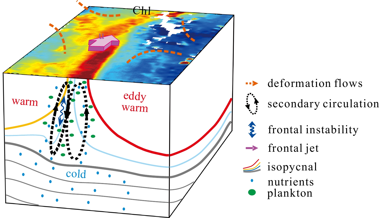
Abstract: Submesoscale activity in the upper ocean has received intense studies through simulations and observations in the last decade, but in the eddy-active South China Sea (SCS) the fine-scale dynamical processes of submesoscale behaviors and their potential impacts have not been well understood. This study focuses on the elongated filaments of an eddy field in the northern SCS and investigates submesoscale-enhanced vertical motions and the underlying mechanism using satellite-derived observations and a high-resolution (~500 m) simulation. The satellite images show that the elongated highly productive stripes with a typical lateral scale of ~25 km and associated filaments are frequently observed at the periphery of mesoscale eddies. The diagnostic results based on the 500 m-resolution realistic simulation indicate that these submesoscale filaments are characterized by cross-filament vertical secondary circulations with an increased vertical velocity reaching O(100 m/d) due to submesoscale instabilities. The vertical advections of secondary circulations drive a restratified vertical buoyancy flux along filament zones and induce a vertical heat flux up to 110 W/m2. This result implies a significant submesoscale-enhanced vertical exchange between the ocean surface and interior in the filaments. Frontogenesis that acts to sharpen the lateral buoyancy gradients is detected to be conducive to driving submesoscale instabilities and enhancing secondary circulations through increasing the filament baroclinicity. The further analysis indicates that the filament frontogenesis detected in this study is not only derived from mesoscale straining of the eddy, but also effectively induced by the subsequent submesoscale straining due to ageostrophic convergence. In this context, these submesoscale filaments and associated frontogenetic processes can provide a potential interpretation for the vertical nutrient supply for phytoplankton growth in the high-productive stripes within the mesoscale eddy, as well as enhanced vertical heat transport.
-
Key words:
- submesoscale process /
- vertical exchange /
- frontogenesis /
- South China Sea
-
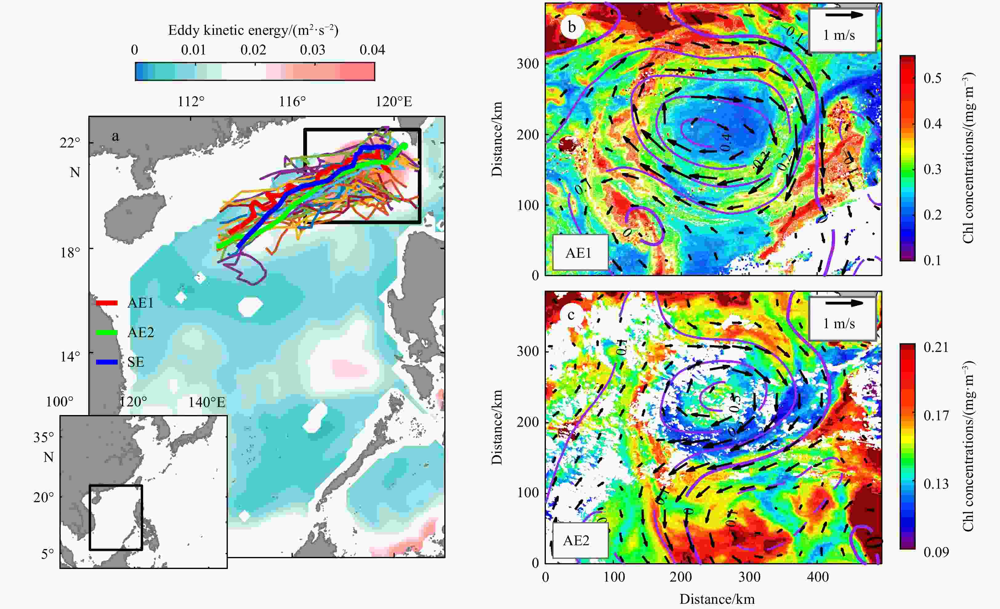
Figure 1. Climatological map of eddy kinetic energy (shading) and the trajectory of mesoscale eddies (color lines) in winter (December, January, February) from 1993 to 2020 in the South China Sea (a); satellite-observed chlorophyll (Chl) concentrations for the AE1 on December 4, 2013 (b) and the AE2 on November 8, 2015 (c). The data in the shelf (<500 m) have been removed. The red, green, and blue bold lines in a show the eddy case trajectory of AE1, AE2 and simulated eddy SE, respectively. Purple contours denote the sea level anomaly and vectors show the geostrophic velocity anomaly. AE1, AE2: anticyclonic eddies.
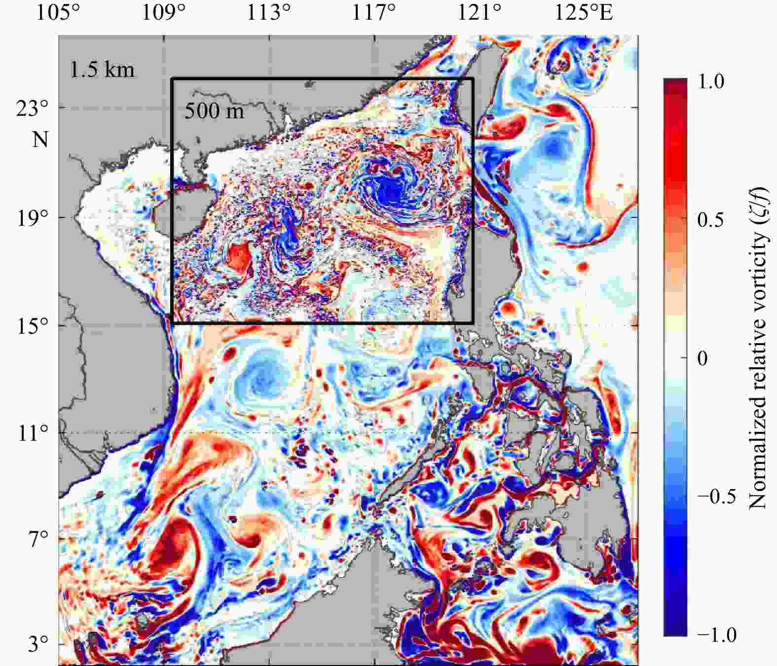
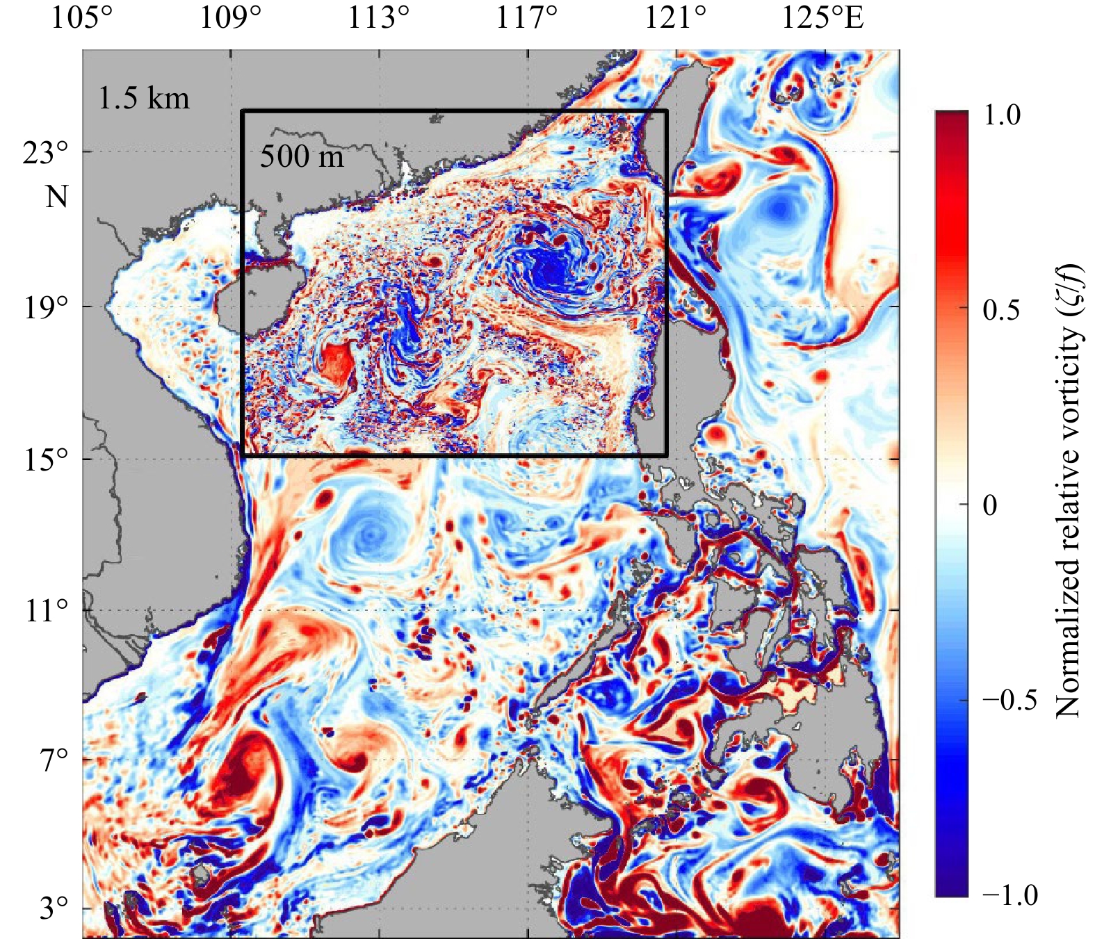
Figure 2. Snapshot of surface Rossby number (
$Ro{\text{ = }}\text{ζ} {\text{/}}f$ ) in the nested South China Sea winter simulations. The resolution of ROMS1 is 1.5 km. The boundary of the second nested domain with ∆x=500 m is delineated by a black box.
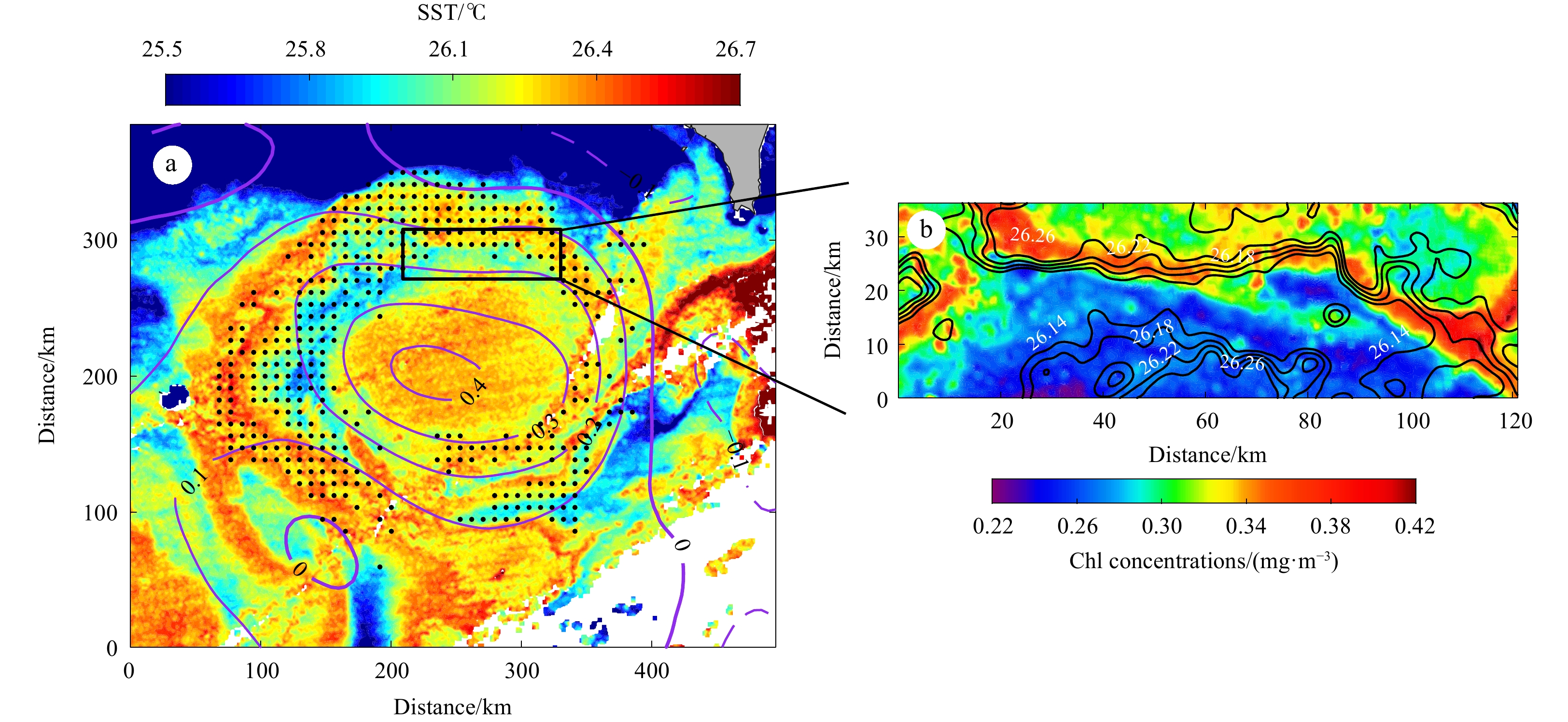
Figure 3. Observed sea surface temperature (SST) field at the time of Fig. 1b (a); snapshot of chlorophyll (Chl) (shading) and SST (contours at an interval of 0.04°C) for the submesoscale filaments (b). Purple contours denote the sea level anomaly. Black spots show the distribution of high-productive filaments (>0.3 mg/m3).
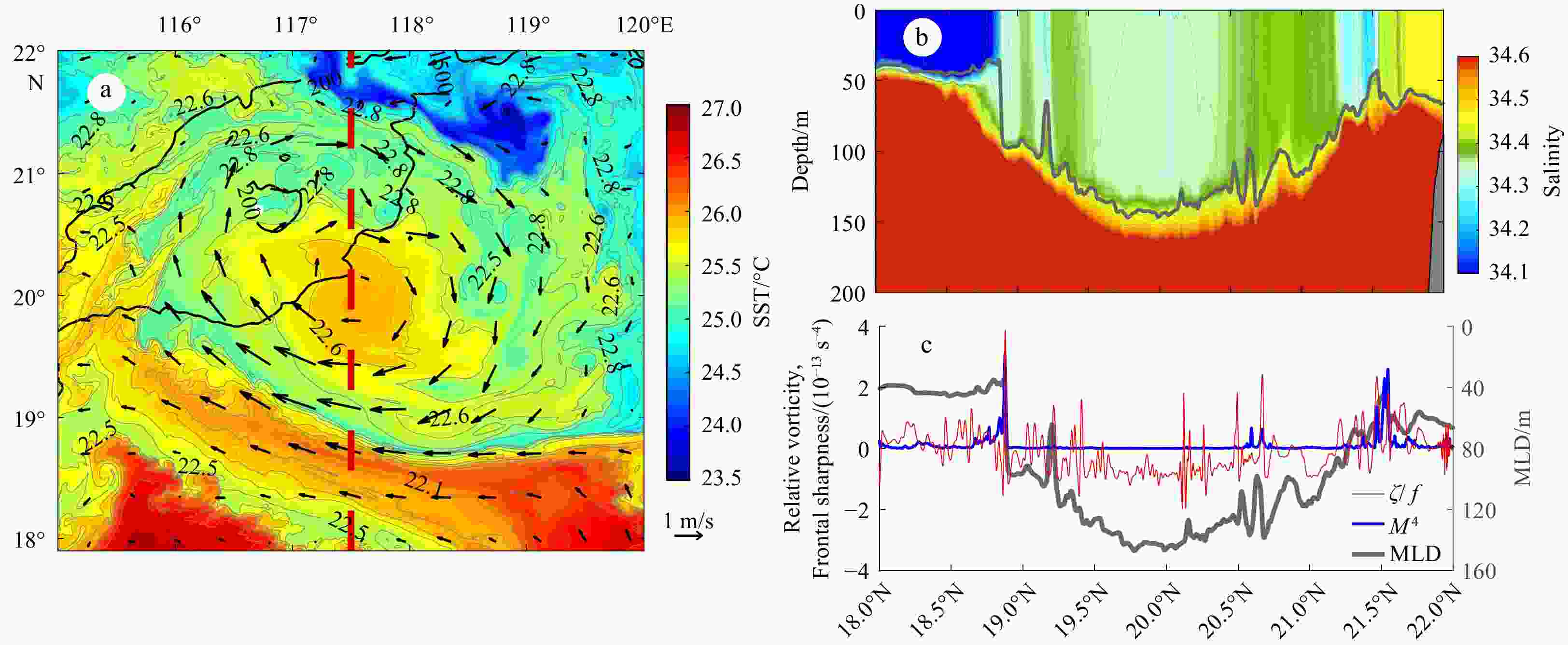
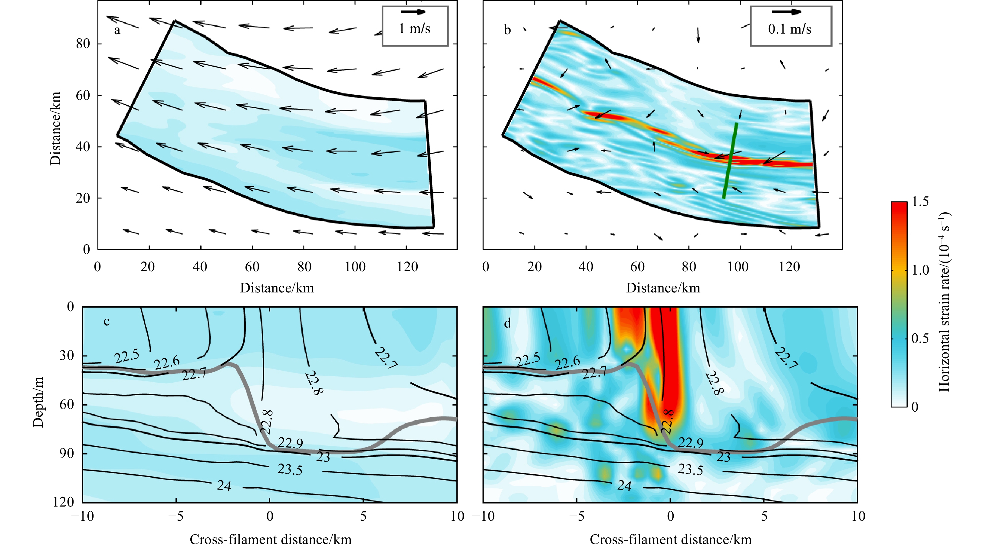
Figure 4. Simulated sea surface temperature (SST) with horizontal velocity (vectors) (a) and a cross-eddy slice of salinity along the 117.5°E section (red dashed lines) (b) on December 18; cross-eddy profiles of normalized relative vorticity
$(\text{ζ} {\text{/}}f)$ and frontal sharpness (M4) averaged over the mixed layer depth (MLD) (c). The isobaths at 200 m and 1 500 m are shown by black contours. Gray contours denote the potential density at an interval of 0.1 kg/m3. The thick gray line denotes the MLD.
Figure 5. Frontal sharpness
$ {M^4} $ (a), strain rate$ St $ (b), relative vorticity$ \zeta $ normalized by$ f $ (c), and normalized divergence${\text{δ} \mathord{\left/ {\vphantom {\delta f}} \right. } f}$ (d) at the surface for the mesoscale eddy shown in Fig. 4. Black contours denote the isobaths at 200 m and 1 500 m. A segment of the strongest filament is outlined by the black box.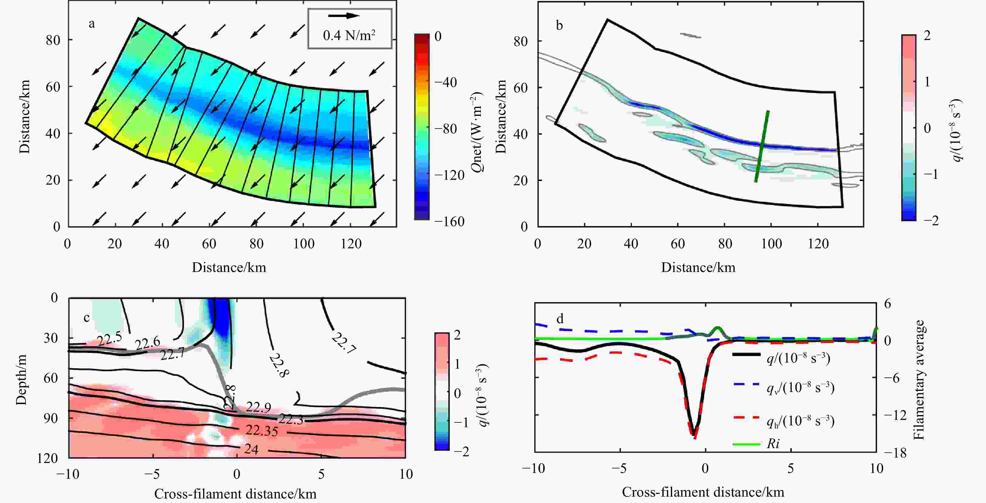
Figure 6. Surface heat flux Qnet (shading) with surface wind stress (vectors) (a); snapshot (b) and vertical section (c) of Ertel potential vorticity (PV)
$ q $ ; filament-averaged profiles of the Ertel PV terms and Richardson number Ri (d). The cross-filament transects (shown at an interval of 30 transects) is represented by cross-filament lines in a. The filament axis is defined by the strongest frontal sharpness. Thin gray contours show the fields of frontal sharpness >1×10⁻¹³ s−4. The isopycnal surfaces are shown by black contours (kg/m3) and the mixed layer depth is denoted by the gray line in c. The segments of$0.25 < Ri < 0.95$ and$Ri > 1$ are shown in dark green and green, respectively.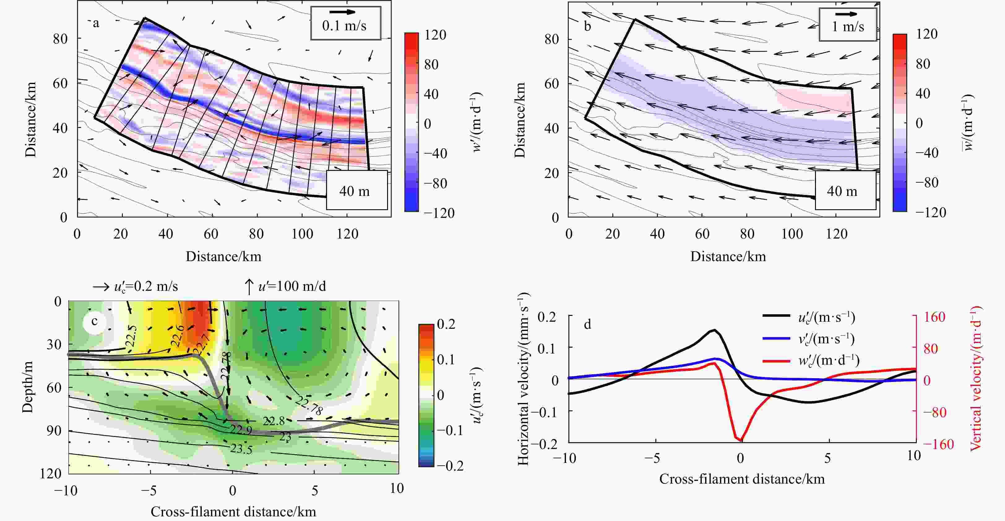
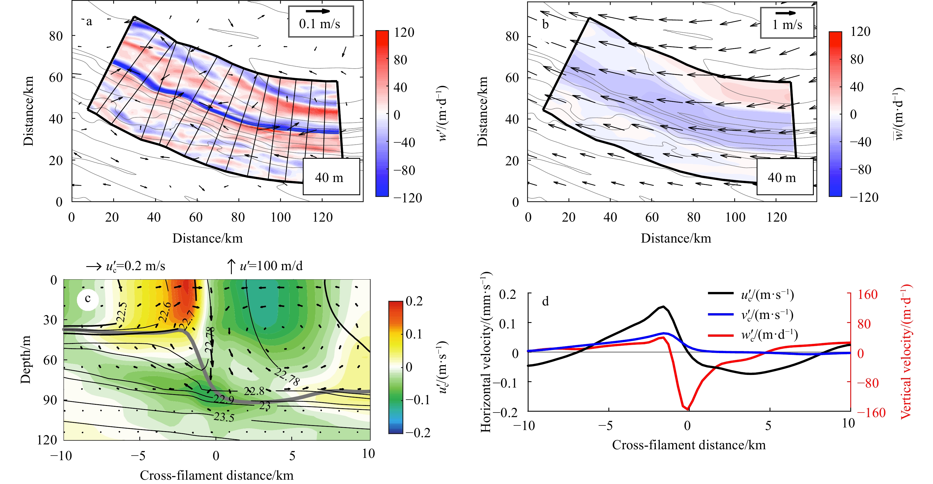
Figure 7. Submesoscale vertical velocity
$ w' $ (a) and mesoscale vertical velocity$\overline w$ (b) at a depth of 40 m; vertical section of submesoscale along-filament velocity$ {u'_{\text{c}}} $ averaged along the filament (c); submesoscale velocity profiles averaged over the mixed layer depth (MLD) in the filamentary region (d). Vectors in a and b denote the surface submesoscale and mesoscale flow, respectively. Gray contours show the potential density at an interval of 0.1 kg/m3. Black contours show the isopycnal surfaces and the gray line denotes the MLD. Vectors at the section show the cross-filament$ {v'_{\text{c}}} $ and vertical velocities$ w' $ at submesoscale.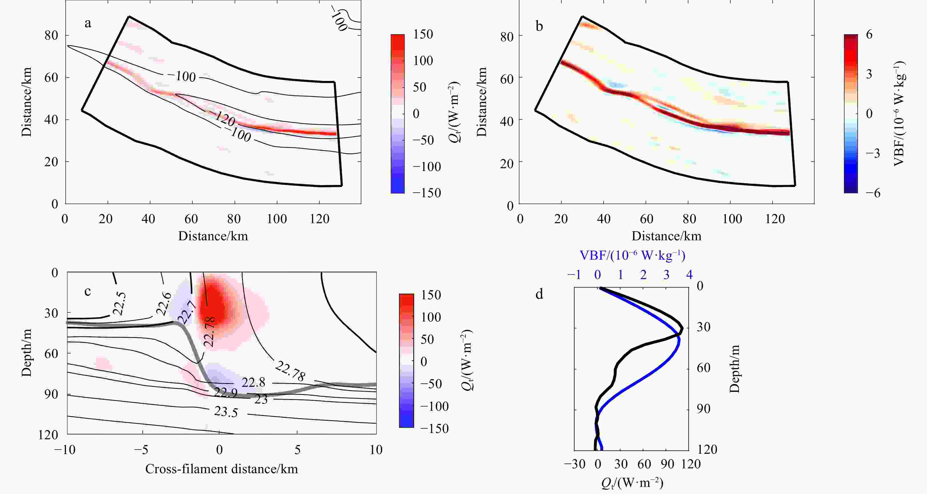
Figure 8. Vertical heat flux
$ {Q_{\text{t}}} $ (a) and vertical buoyancy flux (VBF) (b) averaged over the mixed layer; vertical section of$ {Q_{\text{t}}} $ (shading), potential density (black contours; kg/m3) and the mixed layer depth (gray line) averaged along the filament (c); vertical profiles of$ {Q_{\text{t}}} $ and VBF averaged horizontally in the filamentary region (d). Contours in a denote the surface heat loss$ {Q_{{\text{net}}}} $ .
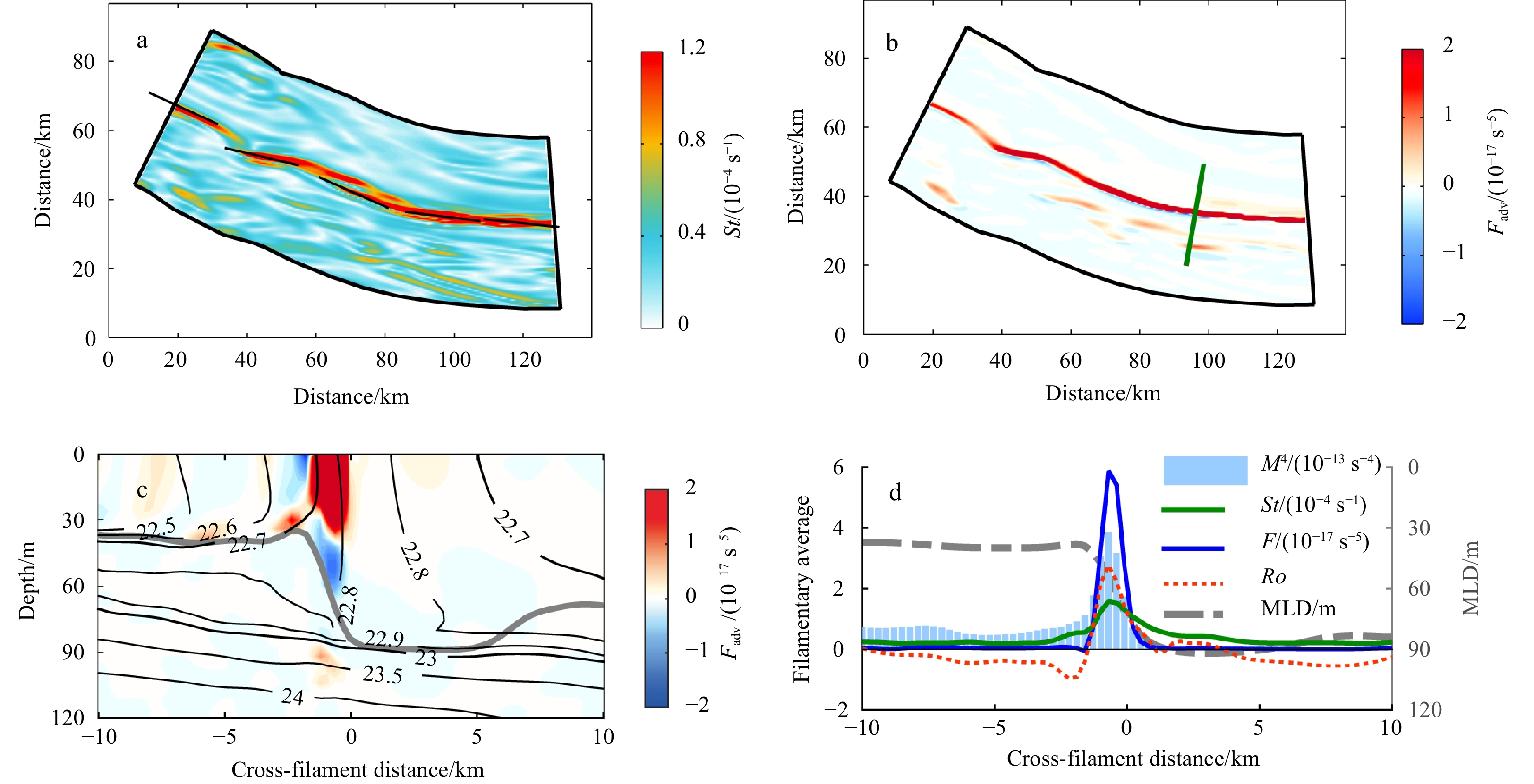
Figure 9. Horizontal strain rate
$ St $ (a) and frontogenetic tendency$ {F_{{\text{adv}}}} $ (b) at the surface; vertical distribution of frontogenetic tendency (shading) and potential density (black contours; kg/m3) along a cross-filament section (the green line in b) (c); instantaneous filament-averaged profiles for the parameters (d). Black lines in a show the direction of the principal strain axis$ {\theta _{\text{p}}} $ . The gray line denotes the mixed layer depth (MLD).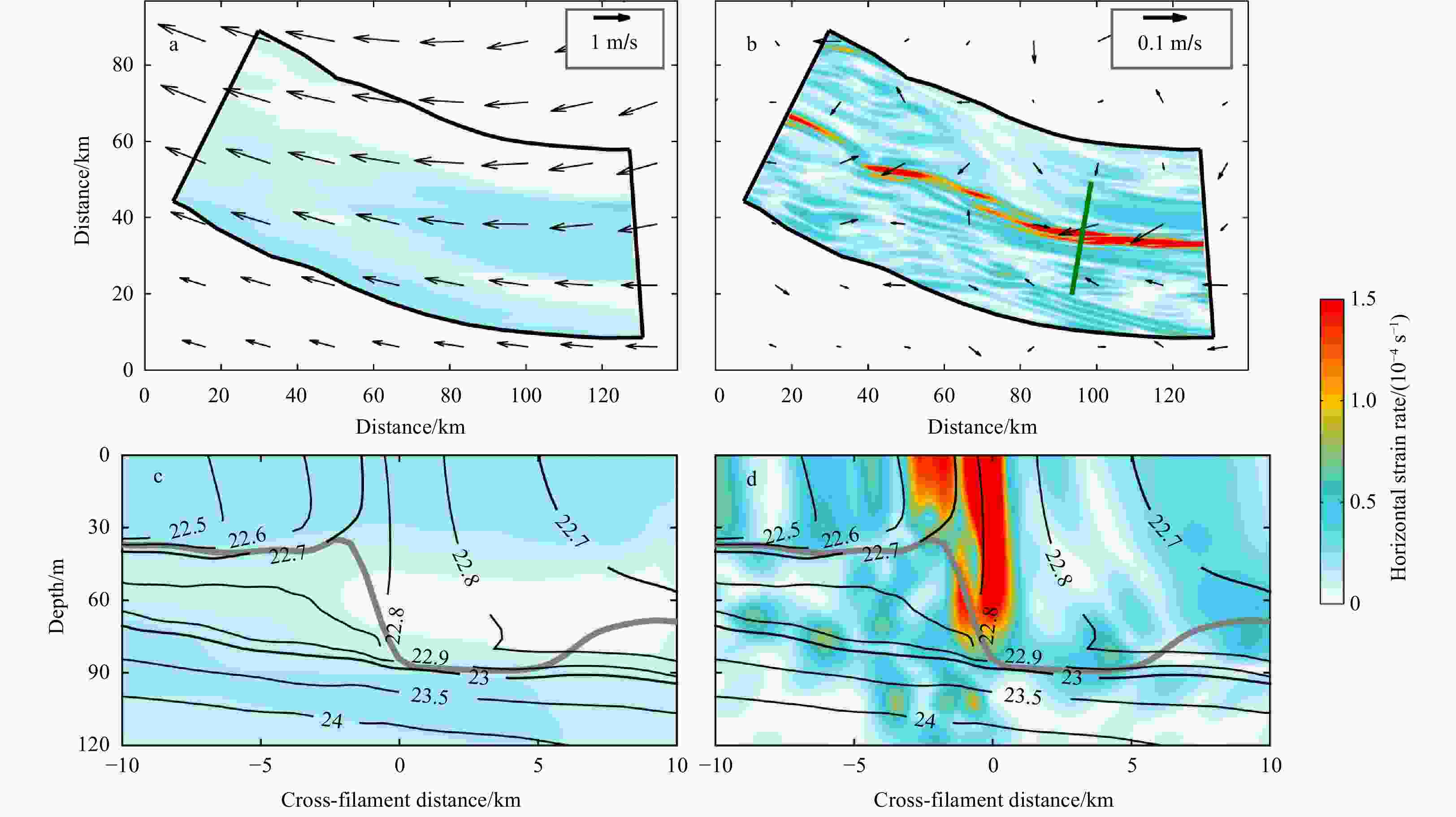
Figure 10. Surface horizontal strain rate associated with mesoscale flows
$ S{t_{\text{m}}} $ (a) and submesoscale flows$ S{t_{\text{s}}} $ (b); cross-filament slices of the$ S{t_{\text{m}}} $ (c) and$ S{t_{\text{s}}} $ (d). The horizontal mesoscale flows and submesoscale perturbations are shown by vectors. Black contours denote the isopycnal surfaces (kg/m3). The mixed layer depth is denoted by the thick gray line.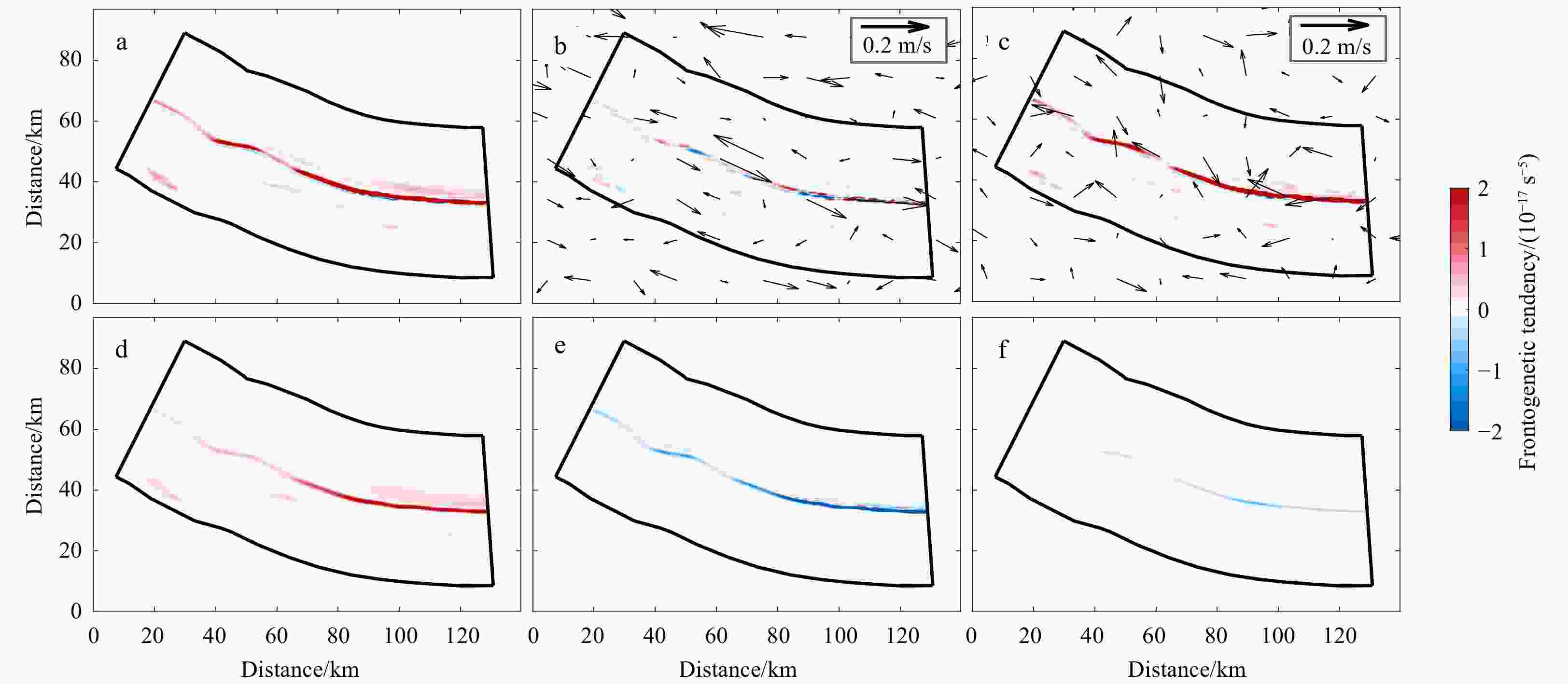
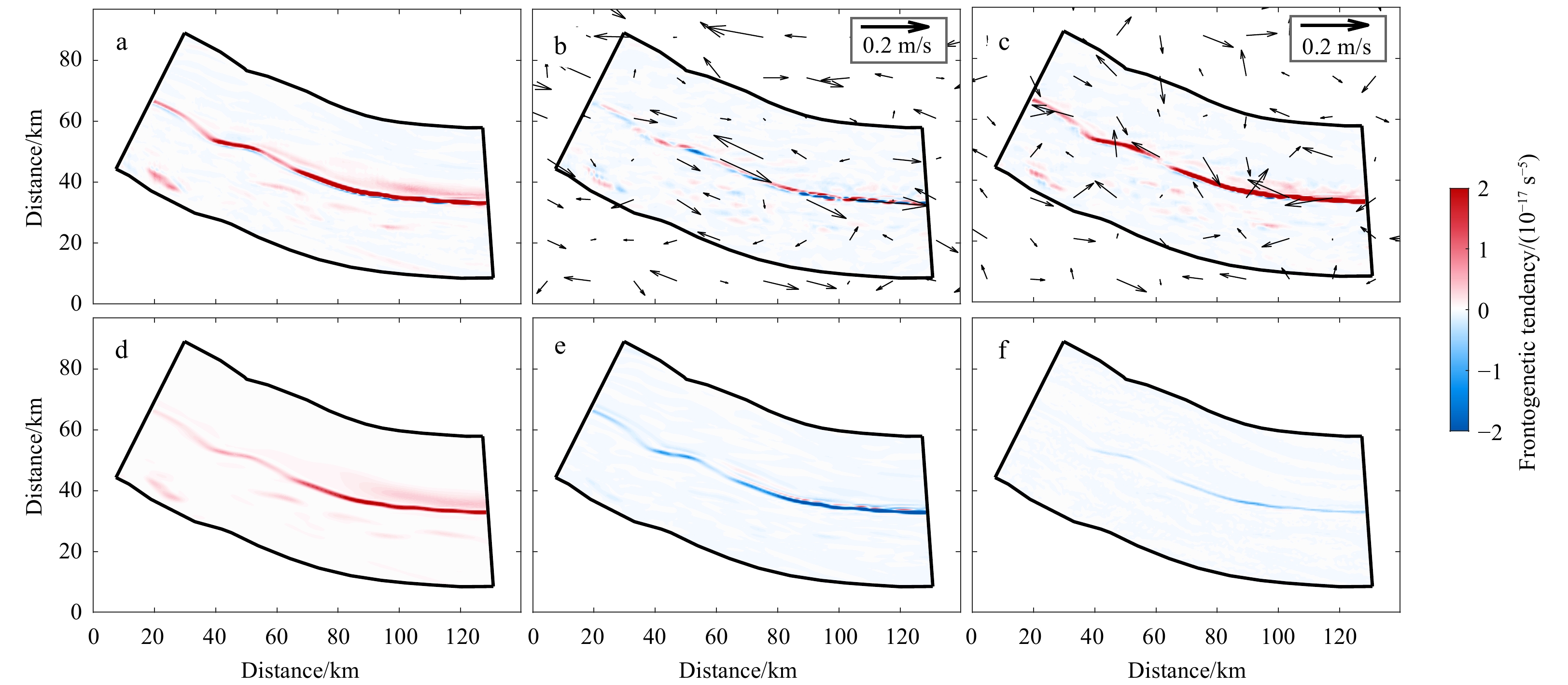
Figure 11. Mixed layer-averaged total frontogenetic tendency F (a) and its terms caused by geostrophic self-straining
${F_{\rm{g}}}$ (b), ageostrophic horizontal advection$ {F_u} $ (c), external straining deformation${F_{{\text{α}}}}$ (d), ageostrophic vertical advection$ {F_w} $ (e), and vertical mixing${F_{{\kappa _{\rm{v}}}}}$ (f). Vectors in b and c show the submesoscale geostrophic and ageostrophic flows, respectively. -
[1] Adams K A, Hosegood P, Taylor J R, et al. 2017. Frontal circulation and submesoscale variability during the formation of a Southern Ocean mesoscale eddy. Journal of Physical Oceanography, 47(7): 1737–1753. doi: 10.1175/JPO-D-16-0266.1 [2] Bachman S D, Fox-Kemper B, Taylor J R, et al. 2017. Parameterization of frontal symmetric instabilities. I: theory for resolved fronts. Ocean Modelling, 109: 72–95. doi: 10.1016/j.ocemod.2016.12.003 [3] Boccaletti G, Ferrari R, Fox-Kemper B. 2007. Mixed layer instabilities and restratification. Journal of Physical Oceanography, 37(9): 2228–2250. doi: 10.1175/JPO3101.1 [4] Brannigan L, Marshall D P, Naveira-Garabato A, et al. 2015. The seasonal cycle of submesoscale flows. Ocean Modelling, 92: 69–84. doi: 10.1016/j.ocemod.2015.05.002 [5] Bryden H L, Brady E C. 1989. Eddy momentum and heat fluxes and their effects on the circulation of the equatorial Pacific Ocean. Journal of Marine Research, 47(1): 55–79. doi: 10.1357/002224089785076389 [6] Capet X, McWilliams J C, Molemaker M J, et al. 2008. Mesoscale to submesoscale transition in the California current system. Part II: Frontal processes. Journal of Physical Oceanography, 38(1): 44–64. doi: 10.1175/2007JPO3672.1 [7] Carton J A, Giese B S. 2008. A reanalysis of ocean climate using simple ocean data assimilation (SODA). Monthly Weather Review, 136(8): 2999–3017. doi: 10.1175/2007MWR1978.1 [8] Chelton D B, DeSzoeke R A, Schlax M G, et al. 1998. Geographical variability of the first baroclinic Rossby radius of deformation. Journal of Physical Oceanography, 28(3): 433–460. doi: 10.1175/1520-0485(1998)028<0433:GVOTFB>2.0.CO;2 [9] Chelton D B, Gaube P, Schlax M G, et al. 2011a. The Influence of nonlinear mesoscale eddies on near-surface oceanic chlorophyll. Science, 334(6054): 328–332. doi: 10.1126/science.1208897 [10] Chelton D B, Schlax M G, Samelson R M. 2011b. Global observations of nonlinear mesoscale eddies. Progress in Oceanography, 91(2): 167–216. doi: 10.1016/j.pocean.2011.01.002 [11] Chen Gengxin, Hou Yijun, Chu Xiaoqing. 2011. Mesoscale eddies in the South China Sea: mean properties, spatiotemporal variability, and impact on thermohaline structure. Journal of Geophysical Research: Oceans, 116(C6): C06018 [12] da Silva A M, Young C C, Levitus S. 1994. Atlas of surface marine data 1994, volume 1: algorithms and procedures. Washington, DC: U. S. Department of Commerce, NOAA, NESDIS [13] D’Asaro E, Lee C, Rainville L, et al. 2011. Enhanced turbulence and energy dissipation at ocean fronts. Science, 332(6027): 318–322. doi: 10.1126/science.1201515 [14] Dauhajre D P, McWilliams J C, Uchiyama Y. 2017. Submesoscale coherent structures on the continental shelf. Journal of Physical Oceanography, 47(12): 2949–2976. doi: 10.1175/JPO-D-16-0270.1 [15] Dong Changming, McWilliams J C, Liu Yu, et al. 2014. Global heat and salt transports by eddy movement. Nature Communications, 5(1): 3294. doi: 10.1038/ncomms4294 [16] Dong Jihai, Zhong Yisen. 2018. The spatiotemporal features of submesoscale processes in the northeastern South China Sea. Acta Oceanologica Sinica, 37(11): 8–18. doi: 10.1007/s13131-018-1277-2 [17] Dong Jihai, Zhong Yisen. 2020. Submesoscale fronts observed by satellites over the northern South China Sea shelf. Dynamics of Atmospheres and Oceans, 91: 101161. doi: 10.1016/j.dynatmoce.2020.101161 [18] Fox-Kemper B, Ferrari R, Hallberg R. 2008. Parameterization of mixed layer eddies. Part I: theory and diagnosis. Journal of Physical Oceanography, 38(6): 1145–1165. doi: 10.1175/2007JPO3792.1 [19] Gula J, Molemaker M J, McWilliams J C. 2014. Submesoscale cold filaments in the Gulf Stream. Journal of Physical Oceanography, 44(10): 2617–2643. doi: 10.1175/JPO-D-14-0029.1 [20] Guo Lin, Xiu Peng, Chai Fei, et al. 2017. Enhanced chlorophyll concentrations induced by Kuroshio intrusion fronts in the northern South China Sea. Geophysical Research Letters, 44(22): 11565–11572. doi: 10.1002/2017GL075336 [21] Hosegood P J, Gregg M C, Alford M H. 2013. Wind-driven submesoscale subduction at the north Pacific subtropical front. Journal of Geophysical Research: Oceans, 118(10): 5333–5352. doi: 10.1002/jgrc.20385 [22] Hoskins B J. 1974. The role of potential vorticity in symmetric stability and instability. Quarterly Journal of the Royal Meteorological Society, 100(425): 480–482. doi: 10.1002/qj.49710042520 [23] Hoskins B J. 1982. The mathematical theory of frontogenesis. Annual Review of Fluid Mechanics, 14: 131–151. doi: 10.1146/annurev.fl.14.010182.001023 [24] Jing Zhiyou, Fox-Kemper B, Cao Haijin, et al. 2021. Submesoscale fronts and their dynamical processes associated with symmetric instability in the northwest Pacific subtropical ocean. Journal of Physical Oceanography, 51(1): 83–100. doi: 10.1175/JPO-D-20-0076.1 [25] Klein P, Lapeyre G. 2009. The oceanic vertical pump induced by mesoscale and submesoscale turbulence. Annual Review of Marine Science, 1: 351–375. doi: 10.1146/annurev.marine.010908.163704 [26] Klein P, Lapeyre G, Roullet G, et al. 2011. Ocean turbulence at meso and submesoscales: connection between surface and interior dynamics. Geophysical & Astrophysical Fluid Dynamics, 105(4−5): 421–437 [27] Klymak J M, Shearman R K, Gula J, et al. 2016. Submesoscale streamers exchange water on the north wall of the Gulf Stream. Geophysical Research Letters, 43(3): 1226–1233. doi: 10.1002/2015GL067152 [28] Lapeyre G, Klein P. 2006. Dynamics of the upper oceanic layers in terms of surface quasigeostrophy theory. Journal of Physical Oceanography, 36(2): 165–176. doi: 10.1175/JPO2840.1 [29] Large W G, McWilliams J C, Doney S C. 1994. Oceanic vertical mixing: a review and a model with a nonlocal boundary layer parameterization. Reviews of Geophysics, 32(4): 363–403. doi: 10.1029/94RG01872 [30] Lévy M, Klein P, Treguier A M. 2001. Impact of sub-mesoscale physics on production and subduction of phytoplankton in an oligotrophic regime. Journal of Marine Research, 59(4): 535–565. doi: 10.1357/002224001762842181 [31] Li Jiajun, Jiang Xin, Li Gang, et al. 2017. Distribution of picoplankton in the northeastern South China Sea with special reference to the effects of the Kuroshio intrusion and the associated mesoscale eddies. Science of the Total Environment, 589: 1–10. doi: 10.1016/j.scitotenv.2017.02.208 [32] Li Ruihuan, Xu Jie, Cen Xianrong, et al. 2021. Nitrate fluxes induced by turbulent mixing in dipole eddies in an oligotrophic ocean. Limnology and Oceanography, 66(7): 2842–2854. doi: 10.1002/lno.11794 [33] Lin Hongyang, Liu Zhiyu, Hu Jianyu, et al. 2020. Characterizing meso- to submesoscale features in the South China Sea. Progress in Oceanography, 188: 102420. doi: 10.1016/j.pocean.2020.102420 [34] Mahadevan A. 2016. The impact of submesoscale physics on primary productivity of plankton. Annual Review of Marine Science, 8: 161–184. doi: 10.1146/annurev-marine-010814-015912 [35] Martin A P. 2003. Phytoplankton patchiness: the role of lateral stirring and mixing. Progress in Oceanography, 57(2): 125–174. doi: 10.1016/S0079-6611(03)00085-5 [36] Mason E, Pascual A, McWilliams J C. 2014. A new sea surface height-based code for oceanic mesoscale eddy tracking. Journal of Atmospheric and Oceanic Technology, 31(5): 1181–1188. doi: 10.1175/JTECH-D-14-00019.1 [37] McGillicuddy D J Jr. 2016. Mechanisms of physical-biological-biogeochemical interaction at the oceanic mesoscale. Annual Review of Marine Science, 8: 125–159. doi: 10.1146/annurev-marine-010814-015606 [38] McGillicuddy D J Jr, Anderson L A, Doney S C, et al. 2003. Eddy-driven sources and sinks of nutrients in the upper ocean: results from a 0.1° resolution model of the North Atlantic. Global Biogeochemical Cycles, 17(2): 1035 [39] McWilliams J C. 2017. Submesoscale surface fronts and filaments: secondary circulation, buoyancy flux, and frontogenesis. Journal of Fluid Mechanics, 823: 391–432. doi: 10.1017/jfm.2017.294 [40] McWilliams J C, Colas F, Molemaker M J. 2009a. Cold filamentary intensification and oceanic surface convergence lines. Geophysical Research Letters, 36(18): L18602. doi: 10.1029/2009GL039402 [41] McWilliams J C, Gula J, Molemaker M J, et al. 2015. Filament frontogenesis by boundary layer turbulence. Journal of Physical Oceanography, 45(8): 1988–2005. doi: 10.1175/JPO-D-14-0211.1 [42] McWilliams J C, Molemaker M J, Olafsdottir E I. 2009b. Linear fluctuation growth during frontogenesis. Journal of Physical Oceanography, 39(12): 3111–3129. doi: 10.1175/2009JPO4186.1 [43] Munk W, Armi L, Fischer K, et al. 2000. Spirals on the sea. Proceedings of the Royal Society A: Mathematical, Physical and Engineering Sciences, 456(1997): 1217–1280 [44] Nan Feng, Xue Huijie, Xiu Peng, et al. 2011. Oceanic eddy formation and propagation southwest of Taiwan. Journal of Geophysical Research: Oceans, 116(C12): C12045. doi: 10.1029/2011JC007386 [45] Omand M M, D’Asaro E A, Lee C M, et al. 2015. Eddy-driven subduction exports particulate organic carbon from the spring bloom. Science, 348(6231): 222–225. doi: 10.1126/science.1260062 [46] Penven P, Debreu L, Marchesiello P, et al. 2006. Evaluation and application of the ROMS 1-way embedding procedure to the central california upwelling system. Ocean Modelling, 12(1–2): 157–187. doi: 10.1016/j.ocemod.2005.05.002 [47] Qiu Bo, Chen Shuiming. 2010. Interannual variability of the North Pacific Subtropical Countercurrent and its associated mesoscale eddy field. Journal of Physical Oceanography, 40(1): 213–225. doi: 10.1175/2009JPO4285.1 [48] Read J F, Pollard R T, Allen J T. 2007. Sub-mesoscale structure and the development of an eddy in the subantarctic front north of the Crozet Islands. Deep-Sea Research Part II: Topical Studies in Oceanography, 54(18–20): 1930–1948. doi: 10.1016/j.dsr2.2007.06.013 [49] Risien C M, Chelton D B. 2008. A global climatology of surface wind and wind stress fields from eight years of QuikSCAT scatterometer data. Journal of Physical Oceanography, 38(11): 2379–2413. doi: 10.1175/2008JPO3881.1 [50] Shakespeare C J, Taylor J R. 2013. A generalized mathematical model of geostrophic adjustment and frontogenesis: uniform potential vorticity. Journal of Fluid Mechanics, 736: 366–413. doi: 10.1017/jfm.2013.526 [51] Shchepetkin A F, McWilliams J C. 2005. The regional oceanic modeling system (ROMS): a split-explicit, free-surface, topography-following-coordinate oceanic model. Ocean Modelling, 9(4): 347–404. doi: 10.1016/j.ocemod.2004.08.002 [52] Spall M A. 1995. Frontogenesis, subduction, and cross-front exchange at upper ocean fronts. Journal of Geophysical Research: Oceans, 100(C2): 2543–2557. doi: 10.1029/94JC02860 [53] Stone P H. 1966. On non-geostrophic baroclinic stability. Journal of the Atmospheric Sciences, 23(4): 390–400. doi: 10.1175/1520-0469(1966)023<0390:ONGBS>2.0.CO;2 [54] Su Zhan, Torres H, Klein P, et al. 2020. High-frequency submesoscale motions enhance the upward vertical heat transport in the global ocean. Journal of Geophysical Research: Oceans, 125(9): e2020JC016544 [55] Su Zhan, Wang Jinbo, Klein P, et al. 2018. Ocean submesoscales as a key component of the global heat budget. Nature Communications, 9(1): 775. doi: 10.1038/s41467-018-02983-w [56] Sullivan P P, McWilliams J C. 2018. Frontogenesis and frontal arrest of a dense filament in the oceanic surface boundary layer. Journal of Fluid Mechanics, 837: 341–380. doi: 10.1017/jfm.2017.833 [57] Tang Qunshu, Jing Zhiyou, Lin Jianmin, et al. 2021. Diapycnal mixing in the subthermocline of the Mariana Ridge from high-resolution seismic images. Journal of Physical Oceanography, 51(4): 1283–1300. doi: 10.1175/JPO-D-20-0120.1 [58] Tarry D R, Essink S, Pascual A, et al. 2021. Frontal convergence and vertical velocity measured by drifters in the Alboran Sea. Journal of Geophysical Research: Oceans, 126(4): e2020JC016614 [59] Taylor J R, Ferrari R. 2009. On the equilibration of a symmetrically unstable front via a secondary shear instability. Journal of Fluid Mechanics, 622: 103–113. doi: 10.1017/S0022112008005272 [60] Thomas L N, Taylor J R, Ferrari R, et al. 2013. Symmetric instability in the Gulf Stream. Deep-Sea Research Part II: Topical Studies in Oceanography, 91: 96–110. doi: 10.1016/j.dsr2.2013.02.025 [61] Thompson A F, Lazar A, Buckingham C, et al. 2016. Open-ocean submesoscale motions: a full seasonal cycle of mixed layer instabilities from gliders. Journal of Physical Oceanography, 46(4): 1285–1307. doi: 10.1175/JPO-D-15-0170.1 [62] Wang Dongxiao, Xu Hongzhou, Lin Jing, et al. 2008. Anticyclonic eddies in the northeastern South China Sea during winter 2003/2004. Journal of Oceanography, 64(6): 925–935. doi: 10.1007/s10872-008-0076-3 [63] Woodruff S D, Worley S J, Lubker S J, et al. 2011. ICOADS Release 2.5: extensions and enhancements to the surface marine meteorological archive. International Journal of Climatology, 31(7): 951–967. doi: 10.1002/joc.2103 [64] Yang Qingxuan, Nikurashin M, Sasaki H, et al. 2019. Dissipation of mesoscale eddies and its contribution to mixing in the northern South China Sea. Scientific Reports, 9(1): 556. doi: 10.1038/s41598-018-36610-x [65] Yang Qingxuan, Zhao Wei, Liang Xinfeng, et al. 2017. Elevated mixing in the periphery of mesoscale eddies in the South China Sea. Journal of Physical Oceanography, 47(4): 895–907. doi: 10.1175/JPO-D-16-0256.1 [66] Zhang Yanwei, Liu Zhifei, Zhao Yulong, et al. 2014. Mesoscale eddies transport deep-sea sediments. Scientific Reports, 4: 5937 [67] Zhang Zhengguang, Qiu Bo. 2020. Surface chlorophyll enhancement in mesoscale eddies by submesoscale spiral bands. Geophysical Research Letters, 47(14): e2020GL088820 [68] Zhang Zhiwei, Tian Jiwei, Qiu Bo, et al. 2016. Observed 3D structure, generation, and dissipation of oceanic mesoscale eddies in the South China Sea. Scientific Reports, 6(1): 24349. doi: 10.1038/srep24349 [69] Zhang Zhiwei, Zhang Yuchen, Qiu Bo, et al. 2020. Spatiotemporal characteristics and generation mechanisms of submesoscale currents in the northeastern South China Sea revealed by numerical simulations. Journal of Geophysical Research: Oceans, 125(2): e2019JC015404 [70] Zheng Quanan, Xie Lingling, Xiong Xuejun, et al. 2020. Progress in research of submesoscale processes in the South China Sea. Acta Oceanologica Sinica, 39(1): 1–13. doi: 10.1007/s13131-019-1521-4 [71] Zhong Yisen, Bracco A, Tian Jiwei, et al. 2017. Observed and simulated submesoscale vertical pump of an anticyclonic eddy in the South China Sea. Scientific Reports, 7(1): 44011. doi: 10.1038/srep44011 -

 下载:
下载:


 点击查看大图

计量
- 文章访问数: 1231
- HTML全文浏览量: 467
- PDF下载量: 145
- 被引次数: 0

