

-
Abstract: Time series measurements (2010–2017) from the Research Moored Array for African–Asian–Australian Monsoon Analysis and Prediction (RAMA) moorings at 15°N, 90°E and 12°N, 90°E are used to investigate the effect of the seasonal barrier layer (BL) on the mixed-layer heat budget in the Bay of Bengal (BoB). The mixed-layer temperature tendency (∂T/∂t) is primarily controlled by the net surface heat flux that remains in the mixed layer (
${Q}^{{'}}$ ) from March to October, while both${Q}^{{'}}$ and the vertical heat flux at the base of the mixed layer ($ {Q}_{h} $ ), estimated as the residual of the mixed-layer heat budget, dominate during winter (November–February). An inverse relation is observed between the BL thickness and the mixed-layer temperature ($ \mathrm{M}\mathrm{L}\mathrm{T} $ ). Based on the estimations at the moorings, it is suggested that when the BL thickness is ≥25 m, it exerts a considerable influence on ∂T/∂t through the modulation of$ {Q}_{h} $ (warming) in the BoB. The cooling associated with$ {Q}_{h} $ is strongest when the BL thickness is ≤10 m with the$ \mathrm{M}\mathrm{L}\mathrm{T} $ exceeding 29°C, while the contribution from$ {Q}_{h} $ remains nearly zero when the BL thickness varies between 10 m and 25 m. Temperature inversion is evident in the BoB during winter when the BL thickness remains ≥25 m with an average MLT<28.5°C. Furthermore,$ {Q}_{h} $ follows the seasonal cycle of the BL at these RAMA mooring locations, with r>0.72 at the 95% significance level.-
Key words:
- barrier layer /
- vertical heat flux /
- temperature inversion /
- Bay of Bengal
-
1. Introduction
The Bay of Bengal (BoB) is a semi-enclosed basin with unique characteristics due to the influence of the Asian monsoon and freshwater influx. It is distinguished by a strongly stratified surface layer and seasonally reversing circulation (Shetye et al., 1996; Schott and McCreary, 2001; Jinadasa et al., 2020) and remote forcing by seasonal winds and waves in the equatorial Indian Ocean (McCreary et al., 1993; Chen et al., 2015). The BoB receives a large quantity of fresh water (~1 030 km3/a) via precipitation and river runoff that exceeds evaporation (Harenduprakash and Mitra, 1988). This freshening makes the surface layer buoyant and maintains the strong stratification in the BoB (Shetye et al., 1996; Agarwal et al., 2012). This strong stratification maintains the stability in the surface layer (Chowdary et al., 2016) and supports the formation of a barrier layer (BL), a unique layer between the base of the mixed layer and the top of the thermocline (Lukas and Lindstrom, 1991; Sprintall and Tomczak, 1992). The formation and variability of the BL have been attributed to the changes related to the shoaling thermocline, Ekman pumping (Thadathil et al., 2008), mixed-layer depth (MLD) (Vinayachandran et al., 2002), and wave propagation in the BoB (Girishkumar et al., 2011). Wind stress acts against the formation of a thicker BL (Bosc et al., 2009) by deepening the mixed layer, whereas the freshwater flux facilitates a thicker BL (Cronin and McPhaden, 2002) by reducing the MLD through stratification at the surface. The presence of a BL restricts the mixing within the mixed layer and affects the sea surface temperature (SST) by reducing the mixing of cool thermocline water in the mixed layer (Vialard and Delecluse, 1998b; Foltz and McPhaden, 2009). Hence, the BL has an important role in the surface mixed-layer heat balance (Lukas and Lindstrom, 1991). Using a model simulation, de Boyer Montegut et al. (2007) suggested that thicker BLs are linked to positive SST anomalies in the northern Indian Ocean. Thus, understanding of BL (seasonal) formation and its variability is important to explain the mixed-layer energy balance in the BoB.
Generally, SST in the BoB remains higher than 28°C (Shenoi et al., 2002) and during the pre-summer monsoon it exceeds 29°C (Pathirana et al., 2020; Pathirana and Priyadarshani, 2020). The seasonality in the BoB is strong and the climatology of SST, MLD, barrier-layer thickness (BLT), and top of thermocline depth (TTD) is presented in Figs 1a and b. SST which also represents the mixed-layer temperature (
$ \mathrm{M}\mathrm{L}\mathrm{T} $ ) is at maximum, with a thinner mixed layer during pre-summer monsoon (March–May). However, the mixed layer is deepest during summer (June–August) in seasonal climatology (Fig. 1a). TTD remains shallow with a thinner barrier-layer during both pre- and post-summer monsoon (September–November), where they reach to maximum during winter (December–February) (Fig. 1b). Thus, the strong seasonality exists in the BoB may play an important role in regulating the heat in the region. Many studies have suggested that the net surface heat flux (${Q}_\mathrm{net}$ ) dominates the mixed-layer heat budget, and McPhaden and Foltz (2013) pointed out the importance of the radiative heat flux, which dominates in${Q}_\mathrm{net}$ in the tropics. In general,${Q}_\mathrm{net}$ in the BoB completes its annual cycle with two positive peaks during the pre- and post-summer monsoon. The heat change in the mixed layer due to the variations in${Q}_\mathrm{net}$ is balanced by the other terms in the mixed-layer heat budget—the horizontal mixed-layer heat advection ($ \mathrm{H}\mathrm{A}\mathrm{d}\mathrm{v} $ ) and the combination of entrainment and vertical turbulent heat fluxes at the base of the mixed layer ($ {Q}_{h} $ ) (Girishkumar et al., 2013). Though there are many studies addressing the mixed-layer heat budget in the BoB (Shenoi et al., 2002; Girishkumar et al., 2013), accurate estimation of$ {Q}_{h} $ still remains as a challenge due to the inconsistency of accurate subsurface observations. Warner et al. (2016) suggested that the subsurface turbulent heat flux during summer cools the surface layer at rates greater than three times that measured during winter in the BoB. Using the Research Moored Array for African–Asian–Australian Monsoon Analysis and Prediction (RAMA) mooring data in the southern BoB (8°N, 90°E), Girishkumar et al. (2011, 2013) suggested that the vertical process (entrainment and vertical diffusion) can warm the mixed layer during winter with the presence of temperature inversion associated with a thicker BL. However, such studies did not discuss in detail the seasonal changes in$ {Q}_{h} $ and its influence on the seasonal mixed-layer heat budget in the BoB. Also, due to the lack of systemic measurements with high temporal resolution in the BoB, previous studies have not examined in detail the seasonal influence of the BL on the mixed-layer heat budget and their relationship. Figure 1. Seasonal climatology of mixed-layer depth (contours, m) (de Boyer Montegut et al., 2004) and sea surface temperature (SST) (colored shading) (Huang et al., 2017) in the Bay of Bengal (BoB) (a); seasonal climatology of barrier-layer thickness (contours, m) and top of thermocline depth (TTD) (colored shading) in the BoB (de Boyer Montegut et al., 2004) (b).
In this study, we provide a more comprehensive description of the effect of the seasonal BL on the mixed-layer heat budget in the BoB, with respect to
$ \mathrm{M}\mathrm{L}\mathrm{T} $ , temperature inversion ($ -\Delta T $ ),$ {Q}_{h} $ , and entrainment using observations at two RAMA mooring stations (12°N, 90°E and 15°N, 90°E) (McPhaden et al., 2009) from January 2010 to December 2017 (Fig. 2). The remainder of this paper is organized as follows. In Section 2, the data and methods used in the analysis are described. Results and discussion are presented in Section 3, followed by a summary in Section 4. Figure 2. Location of the selected RAMA moorings in the Bay of Bengal (a) and the number of Argo profiles at 15°N, 90°E (area marked with red box) (b), 12°N, 90°E (area marked with blue box) (c) used in the present study.
2. Data and methods
Data from multiple sources are used in this study. Daily time series data from January 2010 to December 2017 obtained from the RAMA moorings (
https://www.pmel.noaa.gov/tao/drupal/disdel/ ) deployed at 15°N, 90°E and 12°N, 90°E (Fig. 2) are used to estimate the daily MLD, TTD, BLT, 23°C isothermal layer depth (D23), and the terms in mixed-layer heat budget. The two RAMA moorings are selected based on the data availability compared with the other RAMA moorings located along 90°E in the BoB. Measurements include SST, subsurface temperature and salinity, air temperature, sea-level pressure, wind velocity, relative humidity, and shortwave and longwave radiation. Ocean temperature is measured at 1 m, 5 m, 10 m, 13 m, 20 m, 40 m, 43 m, 60 m, 80 m, 100 m, 120 m, 140 m, 180 m, 300 m, and 500 m. Salinity data are collected at 1 m, 5 m, 10 m, 20 m, 40 m, 60 m, 100 m, and 140 m. During the analysis, we considered the values between 0°C and 36°C for temperature and 20 and 38 for salinity and all the values outside of these ranges were considered as missing values (RAMA data quality control information is available athttps://www.pmel.noaa.gov/gtmba/data-quality-control ). The data for the upper 120 m are interpolated vertically to 1 m intervals using a spline interpolation technique to facilitate the analysis. Furthermore, we utilize data from Argo (http://www.argodatamgt.org/ ), Hybrid Coordinate Ocean Model (HYCOM) (http://apdrc.soest.hawaii.edu/dods/public_data/Model_output/HYCOM/ ), Ocean General Circulation Model for the Earth Simulator (OFES) (Masumoto et al., 2004), climatology (de Boyer Montegut et al., 2004), Optimally-interpolated SST (OISST) (https://www.ncdc.noaa.gov/oisst ), Ocean Surface Current Analysis Real-time (OSCAR) (https://podaac-opendap.jpl.nasa.gov/opendap/allData/oscar/preview/L4/oscar_third_deg/ ), and TropFlux (Kumar et al., 2012) to examine the mixed-layer heat budget at the moorings. The seasonal cycles of each parameter are estimated using a fast Fourier transform analysis technique. The calculated correlation values between different parameters are based on the 95% significance level ($\alpha = 0.05$ ) and the confidence intervals are given within square brackets with correlation values in the text.2.1 Mixed-layer depth and barrier-layer thickness
Assuming that the upper layer of the tropical ocean can undergo significant temperature changes in its diurnal cycle and may influence the thickness of the mixed layer, we estimated the MLD as the depth where the density change is equivalent to a 0.2°C temperature criterion starting from a reference depth of 10 m (de Boyer Montegut et al., 2004). Hence, the estimated MLD is always deeper than 10 m in our results, but it is possible to observe MLDs shallower than 10 m in the BoB, particularly during the months of March–April. However, as we mainly focus on the mean seasonal cycle, we assume that the error introduced at times when the MLD is shallower than 10 m is not significant. The TTD is calculated as the depth where the temperature is 0.2°C lower than the temperature at the 10 m reference depth. Thus our calculation of MLD and TTD is based on a fixed threshold in temperature profiles (de Boyer Montegut et al., 2004). BLT is defined as the difference between TTD and ML (
$\mathrm{B}\mathrm{L}\mathrm{T} = \mathrm{T}\mathrm{T}\mathrm{D} - \mathrm{M}\mathrm{L}\mathrm{D}$ ) (Sprintall and Tomczak, 1992). The Argo data in the selected two regions (14°–16°N, 89°–91°E and 11°–13°N, 89°–91°E, Fig. 2) are averaged to produce the monthly means of MLD and BLT to compare with the observations at the RAMA moorings.2.2 Mixed-layer heat budget
Air–sea fluxes at the mooring locations are computed from the daily winds extrapolated to 10 m height, SST, air temperature, and relative humidity. Latent (
${Q}_\mathrm{L}$ ) and sensible (${Q}_\mathrm{S}$ ) heat fluxes are estimated using the Coupled Ocean-Atmosphere Response Experiment bulk algorithms (Fairall et al., 2003). As only the mooring at 15°N, 90°E had longwave radiation (${Q}_\mathrm{LW}$ ) measurements, net longwave radiation from the TropFlux is used (Kumar et al., 2012) for the mooring at 12°N, 90°E. Net shortwave radiation (${Q}_\mathrm{SW}$ ) is estimated from downwelling shortwave radiation measured at the mooring sites, corrected for albedo (6%) at the surface. Finally, the net heat flux (${Q}_\mathrm{net}$ ) is estimated using Eq. (1) given below:$$ {Q}_\mathrm{net}={Q}_\mathrm{SW}+{Q}_\mathrm{LW}+{Q}_\mathrm{L}+{Q}_\mathrm{S}, $$ (1) with the convention that the heat flux into the ocean is positive. The amount of heat flux that remains in the mixed layer due to air–sea exchange is estimated as
${Q}^{{'}}$ , where${Q}^{{'}} = {Q}_\mathrm{net} - {Q}_\mathrm{pen}$ . Here we consider the penetrative solar radiation (${Q}_\mathrm{pen}$ ) and${Q}_\mathrm{net}$ during the estimation of${Q}^{{'}}$ , and assume that it does not introduce error. The penetrating shortwave radiation below the mixed layer is estimated considering${Q}_\mathrm{pen} = 0.47 \times {Q}_\mathrm{SW}.\mathrm{e}^{-k\cdot\mathrm{MLD}}$ (Jouanno et al., 2011) and a constant e-folding depth of 25 m (k = 0.04).To address the seasonal variability of the mixed-layer heat balance at each mooring location, we consider the following expression (Rao and Sivakumar, 2000; Foltz and McPhaden, 2009; Girishkumar et al., 2013):
$$ \frac{\partial T}{\partial t}=\frac{{{Q}^{{'}}}_{}}{\rho {C}_{p}\cdot\mathrm{MLD}}-\left[u\frac{\partial T}{\partial x}+v\frac{\partial T}{\partial y}\right]+{Q}_{h} . $$ (2) The terms in Eq. (2) represent, from left to right, mixed-layer temperature tendency (
$\partial T/\partial t$ ), net surface heat flux that remains in the mixed layer, horizontal mixed-layer$ \mathrm{H}\mathrm{A}\mathrm{d}\mathrm{v} $ , and the combination of entrainment and vertical turbulent heat fluxes at the base of the mixed layer ($ {Q}_{h} $ ). However, when$ {Q}_{h} $ is estimated as the residual of the mixed-layer heat budget, the term also includes errors in the estimation of the other terms in Eq. (2), which are associated with data sources and unrepresented/unresolved physical processes (Foltz and McPhaden, 2009). In Eq. (2),$ T $ is the averaged$ \mathrm{M}\mathrm{L}\mathrm{T} $ ,$ \rho $ is density of seawater ($\rho =$ $1\;024\;\mathrm{k}\mathrm{g}/\mathrm{m}^{3}$ ),$ {C}_{p} $ is specific heat capacity of seawater (${C}_{p} = 4\;000\;\mathrm{J}/ $ $\left({\mathrm{kg} \cdot \mathrm{K}}\right)$ ), and$ t $ is time.${Q}^{{'}}$ at the mooring locations are estimated using the terms in Eq. (1) and${Q}_\mathrm{pen}$ .$ \mathrm{H}\mathrm{A}\mathrm{d}\mathrm{v} $ is estimated using the zonal (u) and meridional (v) components of the surface current measurements from OSCAR with OISST. OISST and$ \mathrm{M}\mathrm{L}\mathrm{T} $ at 12°N (15°N), 90°E shows a reasonably good agreement with a correlation of$r = 0.97$ and a confidence interval of [0.96, 0.98] at the 95% significance level ($r = 0.98$ [0.97, 0.99]), and root mean square difference ($ \mathrm{R}\mathrm{M}\mathrm{S}\mathrm{E} $ ) of 0.2 (0.18)°C. OISST averaged over 50 km on either side of the mooring locations is used to estimate the horizontal gradient of SST (Vialard et al., 2008). The direct estimation of$ {Q}_{h} $ is tricky due to the uncertainties associated with the vertical resolution of temperature observations, the choice of thermocline depth, and the vertical diffusion coefficient. Hence, we estimate$ {Q}_{h} $ as the difference between the observed$\partial T/\partial t$ and the sum of${Q}^{{'}}/\rho {C}_{p}\cdot \text{MLD}$ and horizontal advection (Foltz and McPhaden, 2009). However, to identify the influence of BLT on$ {Q}_{h} $ , we examine the change in entrainment and vertical velocity at the moorings.2.3 Entrainment and vertical velocity
To determine the importance of entrainment in the mixed-layer heat budget, we used the expression
${Q}_{h} = H\left[{W}_{h}+\dfrac{\mathrm{d}h}{\mathrm{d}t}\right]\times \dfrac{\mathrm{MLT}-{T}_{h}}{\mathrm{MLD}} + \varepsilon$ following Girishkumar et al. (2013), where$ {W}_{h} $ is the rate of change of thermocline depth and$\dfrac{\mathrm{d}h}{\mathrm{d}t}$ is the rate of change in MLD,$ {T}_{h} $ is the temperature below 5 m from the MLD, and$\varepsilon$ represents the summation of vertical diffusion and other unresolved processes.$ H $ is the logical operator, which is set to one if${W}_{h}+\dfrac{\text{d}h}{\text{d}t} > 0$ , otherwise it is set to zero, when considering only the upward movement of subsurface water. Entrainment is estimated considering two depth levels,${W}_{h} = \mathrm{T}\mathrm{T}\mathrm{D}$ and${W}_{h} = \mathrm{D}23$ , to examine the variations associated with the selection of thermocline depth. Seasonal change in vertical velocity at the base of the mixed layer,$ \mathrm{T}\mathrm{T}\mathrm{D} $ , and$ \mathrm{D}23 $ are examined using daily data (2010–2014) from OFES. As we are focusing on only the upward movement of the water (entrainment), the negative vertical velocity values are removed before estimating the seasonal cycle.3. Results and discussion
3.1 Seasonal MLD and BLT at the RAMA moorings
The accuracy of the estimated seasonal MLD and BLT is important to enhance the accuracy of the calculated mixed-layer heat budget terms at the RAMA moorings. Therefore, the estimated MLD and BLT from the mooring data are compared with the estimations from Argo, HYCOM, and climatology from de Boyer Montegut et al. (2004), and the results are presented in Fig. 3. However, here we mainly focused on the correlation values rather than the
$ \mathrm{R}\mathrm{M}\mathrm{S}\mathrm{E} $ . At 15°N, 90°E, the MLD correlations are positive, in which the highest correlation ($r = 0.86 \left[0.58, 0.96\right]$ ) is observed between the MLDs from RAMA and Argo with a$\mathrm{R}\mathrm{M}\mathrm{S}\mathrm{E} = 3.7\;\mathrm{m}$ (Fig. 3a). Though a good positive correlation ($r = 0.77 \left[0.35,0.93\right]$ ) exists between MLDs from RAMA and the climatology, from July to December the RAMA mooring at 15°N, 90°E underestimates the MLD compared with the climatology, leading to a$\mathrm{R}\mathrm{M}\mathrm{S}\mathrm{E} = 11.7\;\mathrm{m}$ . The BLT at 15°N, 90°E is strongly positively correlated between each dataset, and the highest correlation ($r = 0.96 \left[0.86,0.98\right]$ ) is between the BLT from RAMA and the climatology with$\mathrm{R}\mathrm{M}\mathrm{S}\mathrm{E} = 5.7\;\mathrm{m}$ (Fig. 3b). At 12°N, 90°E, MLD shows a strong postive correlation ($r > 0.80$ ), but compared with MLD from Argo and climatology, the MLD from HYCOM shows the best agreement ($r = 0.90 \left[0.67,0.97\right]$ ) with MLD from RAMA ($\mathrm{R}\mathrm{M}\mathrm{S}\mathrm{E} = 4\;\mathrm{m}$ ). Similar to that at 15°N, 90°E from July to December, the RAMA mooring at 12°N, 90°E underestimates the MLD compared with the climatology, leading to a$\mathrm{R}\mathrm{M}\mathrm{S}\mathrm{E} = 11.8\;\mathrm{m}$ (Fig. 3c). However, the differences in MLDs from RAMA and climatology during July to December could be attributed to the changes in vertical salinity distribution rather than temperature at the moorings. The BLT at 12°N, 90°E is also strongly positively correlated between each dataset, and the highest correlation ($r = 0.95 $ $\left[0.82,0.98\right]$ ) is between the BLT from RAMA and HYCOM with$\mathrm{R}\mathrm{M}\mathrm{S}\mathrm{E} = 5\;\mathrm{m}$ (Fig. 3d). Thus, the good correlations for MLD and BLT calculated using RAMA data compared with Argo and climatology enhance the validity of using RAMA data in this study (Table 1). Figure 3. Comparison of estimated mixed-layer depth (MLD) (a, b) and the barrier-layer thickness (BLT) (c, d) using observations at the RAMA moorings, Argo, HYCOM, and monthly climatology at 15°N, 90°E (a, c) and 12°N, 90°E (b, d). The numbers represent the correlation (r) values between the RAMA estimations with Argo (red), HYCOM (blue), and climatology (green). The standard deviations of the RAMA observations are: ±6.5 (a), ±8.6 (b), ±16 (c), and ±7.4 (d).Table 1. Correlations at the 95% significance level between the estimations from RAMA data and other data sources
Parameter Data source 15°N, 90°E 12°N, 90°E r RMSE r RMSE MLD RAMA-Argo 0.86 [0.58, 0.96] 3.70 0.82 [0.48, 0.94] 8.00 RAMA-HYCOM 0.42 [0.36, 0.52] 7.20 0.90 [0.67, 0.97] 4.00 RAMA-Climatology 0.77 [0.35, 0.93] 11.75 0.80 [0.42, 0.94] 11.80 BLT RAMA-Argo 0.95 [0.85, 0.98] 5.60 0.77 [0.36, 0.93] 4.90 RAMA-HYCOM 0.85 [0.55, 0.95] 12.50 0.95 [0.82, 0.98] 5.00 RAMA-Climatology 0.96 [0.86, 0.98] 5.70 0.88 [0.63, 0.97] 7.40 MLT RAMA-Argo 0.98 [0.95, 0.99] 0.19 0.88 [0.62, 0.97] 0.70 RAMA-HYCOM 0.98 [0.93, 0.99] 0.51 0.92 [0.73, 0.98] 0.62 RAMA-OISST 0.98 [0.97, 0.99] 0.18 0.97 [0.96, 0.98] 0.20 MLS RAMA-Argo 0.81 [0.45, 0.94] 0.23 0.89 [0.65, 0.97] 0.32 RAMA-HYCOM 0.62 [0.08, 0.88] 0.30 0.91 [0.71, 0.97] 0.20 Note: The confidence intervals are noted in square brackets. MLD: mixed-layer depth; BLT: barrier-layer thickness; MLT: mixed-layer temperature; MLS: mixed-layer salinity. | Show Table DownLoad:
CSV
DownLoad:
CSV
The MLD follows a strong seasonal cycle at the moorings with deepening (summer and winter monsoon) and shoaling (pre- and post-summer monsoon) responding to the seasonal changes. However, a strong seasonality of BLT is observed only at 15°N, 90°E compared with the change in BLT at 12°N, 90°E. The change in the seasonal cycle of BLT at 15°N, 90°E is ~60 m, which is relatively large compared with that at 12°N, 90°E (~30 m) (Thadathil et al., 2007). The differences in BLT at the moorings are relatively large during the winter monsoon (November–February) and this highlights the possible influence from temperature changes in the upper waters. A shallow MLD and a weaker BL are evident during the pre- and post-summer monsoon at both locations, but they are still prominent during the pre-summer monsoon. At the times when the summer monsoon peaks (month of July), the MLD reaches its maximum depth in the seasonal cycle with an average BLT of around 10 m. In agreement with Narvekar and Kumar (2006), the estimated MLD (~40 m) is relatively deep with a thinner BL (~20 m) at 12°N, 90°E compared to that at 15°N, 90°E during winter. In agreement with previous studies (Girishkumar et al., 2011; Felton et al., 2014), the variations in the seasonal cycles of MLD and BLT at the RAMA moorings indicate the relative importance of subsurface temperature and salinity distribution, and surface winds in the BoB. Hence, the relative importance of the seasonality in
$ \mathrm{M}\mathrm{L}\mathrm{T} $ and mixed-layer salinity ($ \mathrm{M}\mathrm{L}\mathrm{S} $ ) at the moorings are discussed in the next section.3.2 Seasonal MLT and MLS at the RAMA moorings
The correct estimation of the seasonal MLT is important as it is used to calculate the
$\partial T/\partial t $ . The accuracy of the estimated MLT could influence$ {Q}_{h} $ , when it is estimated as the residual of the mixed-layer heat budget. Furthermore, the correct estimations of both seasonal MLT and MLS will enhance the validity of using observations at the RAMA moorings to examine the effect of the seasonal BL on the mixed-layer heat budget. Hence, we compare the MLT and MLS at the RAMA moorings with other data sources and the results are presented in Fig. 4. Similar to Section 3.1, here we mainly focus on correlation values. The MLT estimated using mooring data is strongly positively correlated ($r > 0.98 \left[0.96,0.99\right]$ ) with Argo and OISST, where the RMSE (0.18 and 0.20 (°C)) shows relatively good agreement between RAMA MLT and OISST. Further, the MLS estimated from RAMA data shows relatively good agreement with Argo data at 12°N, 90°E ($r = 0.89 \left[0.65,0.97\right],\mathrm{R}\mathrm{M}\mathrm{S}\mathrm{E} = 0.32$ ) and 15°N, 90°E ($r = 0.81 [0.45, 0.94], \mathrm{R}\mathrm{M}\mathrm{S}\mathrm{E} = 0.23$ ). Thus, the observed good correlations for MLT and MLS between RAMA data and Argo data confirm the validity of using RAMA data in this study (Table 1). Figure 4. Comparison of estimated seasonal cycle of mixed-layer temperature (MLT) (a, b) and mixed-layer salinity (MLS) (c, d) using observations at the RAMA moorings, Argo, HYCOM, and OISST at 15°N, 90°E (a, c) and 12°N, 90°E (b, d). The standard deviations of the RAMA observations are: ±0.9 (a), ±0.7 (b), ±0.2 (c), and ±0.3 (d).
The observed seasonality in
$ \mathrm{M}\mathrm{L}\mathrm{T} $ at 15°N, 90°E is relatively strong compared with that at 12°N, 90°E. The seasonal changes in$ \mathrm{M}\mathrm{L}\mathrm{T} $ indicate the presence of a warmer mixed layer during pre- to post-summer monsoon and a cooler mixed layer during winter at the moorings. Furthermore, the$ \mathrm{M}\mathrm{L}\mathrm{T} $ change within the seasonal cycle is obvious from post- to pre-summer monsoon, where the change in$ \mathrm{M}\mathrm{L}\mathrm{T} $ remains almost zero during the summer monsoon. The$ \mathrm{M}\mathrm{L}\mathrm{T} $ , which remains around 29°C between July and September, indicates that the variability of the mixed-layer heat budget terms are limited to post- to pre-summer monsoon in the BoB (Figs 4a, b). The seasonality of$ \mathrm{M}\mathrm{L}\mathrm{S} $ is relatively strong at 15°N, 90°E, where it peaks during late-summer monsoon and remains at a minimum during the pre-summer monsoon in the BoB (Figs 4c, d). Furthermore, it is evident from the results that the$ \mathrm{M}\mathrm{L}\mathrm{S} $ is positively correlated with the MLD, while the$ \mathrm{M}\mathrm{L}\mathrm{T} $ is significantly negatively correlated with the BLT at the moorings (Table 2). Thus, based on the correlations, it is noted that the$ \mathrm{M}\mathrm{L}\mathrm{T} $ is linked with the seasonality of the BLT at 15°N, 90°E, while both$ \mathrm{M}\mathrm{L}\mathrm{T} $ and$ \mathrm{M}\mathrm{L}\mathrm{S} $ are linked with the seasonal cycle of the BLT at 12°N, 90°E in the BoB. The relationship between the BLT and entrainment cooling/heating in the heat budget has been well discussed for the western Pacific (Vialard and Delecluse, 1998b) and tropical North Atlantic (Foltz and McPhaden, 2009). The effect of the seasonal BL on the mixed-layer heat budget in the BoB, with respect to$ \mathrm{M}\mathrm{L}\mathrm{T} $ , temperature inversion ($ -\Delta T $ ),$ {Q}_{h} $ , and entrainment, is discussed in the next section.Table 2. Correlations at the 95% significance level between the estimated barrier-layer thickness (BLT) and several selected parameters at the RAMA moorings15°N, 90°E 12°N, 90°E BLT-MLT −0.86 [−0.88, −0.83] −0.96 [−0.97, −0.95] BLT-HAdv −0.54 [−0.61, −0.47] −0.11 [−0.21, −0.01] BLT-Qh 0.72 [0.67, 0.77] 0.78 [0.74, 0.82] BLT-(Wh=TTD) 0.98 [0.97, 0.99] 0.88 [0.85, 0.90] BLT-(Wh=D23) 0.97 [0.96, 0.98] 0.79 [0.74, 0.83] BLT-(–ΔT) 0.94 [0.93, 0.95] 0.94 [0.92, 0.96] Note: The confidence intervals are noted in square brackets. MLT: mixed-layer temperature; TTD: top of thermocline depth. | Show TableDownLoad:
CSV
3.3 Seasonal mixed-layer heat budget at the RAMA moorings
Consistent with previous studies,
${Q}_\text{net}$ dominates in the mixed-layer heat budget in the BoB (McPhaden and Foltz, 2013). Considering the seasonality of the mixed-layer heat budget terms and based on the data availability we have selected two RAMA moorings. The results are presented in Fig. 5. In general,${Q}_\text{SW}$ and${Q}_\text{L}$ play a primary role in heat gain and loss in${Q}_\text{net}$ compared with that of${Q}_\text{LW}\,\,\mathrm{a}\mathrm{n}\mathrm{d}\,\,{Q}_\text{S}$ . The contribution of${Q}_\text{SW}$ to${Q}_\text{net}$ is deepest during pre- and post-summer monsoon. At 15°N, 90°E,${Q}_\text{SW}$ peaks during pre- and post-summer monsoon with a positive heat gain while the heat loss from${Q}_\text{pen}$ increases compared with that of${Q}_\text{L}$ , which may be attributed to the seasonality of MLD (thin) and surface winds (weak) (Fig. 5a) (Girishkumar et al., 2013). Such seasonal changes are not prominent at 12°N, 90°E except during the pre-summer monsoon, and this further highlights the weakening of seasonality towards the southern BoB (Fig. 5b). Figure 5. Seasonal cycles of turbulent and radiative heat fluxes (a, b) and mixed-layer heat budget terms (c, d) at 15°N, 90°E (a, c) and 12°N, 90°E (b, d) in the Bay of Bengal. The specific terms and their color notations are given in the legend. The standard deviations of the estimated heat budget terms are:
$\partial T/ \partial t = \pm 0.02,{Q}^{{'}} = \pm 0.06,\mathrm{H}\mathrm{A}\mathrm{d}\mathrm{v} = \pm 0.006,\;\mathrm{a}\mathrm{n}\mathrm{d}\;{Q}_{h} = \pm 0.04$ (c), and$\partial T/ \partial t = \pm 0.02,{Q}^{{'}} = \pm 0.03, $ $ \mathrm{H}\mathrm{A}\mathrm{d}\mathrm{v} = \pm 0.007,\;\mathrm{a}\mathrm{n}\mathrm{d}\;{Q}_{h} = \pm 0.02$ (d).The mixed-layer heat budget terms at 15°N, 90°E illustrate a strong seasonality compared with that at 12°N, 90°E (Figs 5c, d). At 15°N, 90°E,
$\partial T/ \partial t $ remains positive (heat gain) during pre- to early summer (March–June), and deviates around zero (~0°C/d) during summer to post-summer monsoon (July–October). Then negative values during winter (November–February) complete its annual cycle. The seasonality of$\partial T/ \partial t $ is relatively weak at 12°N, 90°E and the contribution from$ \mathrm{H}\mathrm{A}\mathrm{d}\mathrm{v} $ at the mooring is also weak. This indicates that the seasonal cycle of the mixed-layer heat budget is mainly influenced by${Q}_\text{net}$ and${Q}_h$ in the BoB. The magnitudes (°C/d) of the mixed-layer heat budget terms remain almost the same during pre- to post-summer monsoon at the moorings, while${Q}^{{'}}/ \rho {C}_{p}.\; \text{MLD}$ varies by ~1°C/d during winter. The influence of${Q}_h$ on the mixed-layer heat budget is higher (positive) during winter and it strengthens towards the northern BoB. The${Q}_h$ , which represents the vertical heat exchange at the base of the mixed layer (entrainment and vertical diffusion), shows positive and negative contributions during November–December and March–June, respectively. As the positive relation between BLT and${Q}_\text{h}$ has been discussed in previous studies (Vialard and Delecluse, 1998a; Foltz and McPhaden, 2009; Girishkumar et al., 2013), it highlights the relative importance of examining the effects of the seasonal BL on the mixed-layer heat budget in the BoB with respect to oceanic process.3.4 Effect of seasonal BLT on
$ \boldsymbol{M}\boldsymbol{L}\boldsymbol{T} $ ,$ \boldsymbol{H}\boldsymbol{A}\boldsymbol{d}\boldsymbol{v} $ and${{{\boldsymbol{Q}}}}_{{{\boldsymbol{h}}}}$ The seasonal cycle of SST (or its proxy,
$ \mathrm{M}\mathrm{L}\mathrm{T} $ ) is driven primarily by the seasonal winds over the BoB, as shown by de Boyer Montegut et al. (2007). Furthermore, they show that the absence or weaker upwelling is another major factor for the observed warmer SSTs in the region. Such findings highlight the presence of stable water layers in the BoB, which is also evident from the variations in the BLT. The average BLT and its seasonality increases towards the northern BoB along 90°E (Thadathil et al., 2007), which also suggests an increase in water column stability. Hence, the spatial and temporal variability of BLT could exert a considerable effect on the mixed-layer heat budget terms in the BoB.BLT shows a significant negative correlation with
$ \mathrm{M}\mathrm{L}\mathrm{T} $ , compared to that with$ \mathrm{M}\mathrm{L}\mathrm{S} $ at the RAMA moorings and the results are presented in Fig. 6a and Table 2. However, from pre- to post-summer,$ \mathrm{M}\mathrm{L}\mathrm{T} $ at the moorings does not show larger differences similar to the changes in BLT. Thus, the observed$ \mathrm{M}\mathrm{L}\mathrm{T} $ variability during pre- to post-summer monsoon may be due to the atmospheric forcing, while oceanic processes (entrainment and vertical diffusion) may play an important role determining the$ \mathrm{M}\mathrm{L}\mathrm{T} $ variability during winter. The relationship between the seasonal cycle of BLT and$ \mathrm{H}\mathrm{A}\mathrm{d}\mathrm{v} $ remains less significant at the moorings (Fig. 6b, Table 2) and indicates that the influence of stratification below the mixed layer on$ \mathrm{H}\mathrm{A}\mathrm{d}\mathrm{v} $ is negligible at the moorings. However, there is a lack of zonal and meridional current observations at the moorings to support examination of the influence of stratification on$ \mathrm{H}\mathrm{A}\mathrm{d}\mathrm{v} $ . Figure 6. Seasonal variability of barrier-layer thickness (BLT) and mixed-layer temperature (MLT) (a), mixed-layer
$ \mathrm{H}\mathrm{A}\mathrm{d}\mathrm{v} $ (b), and$ {Q}_{h} $ (c) at 15°N, 90°E (solid lines) and 12°N, 90°E (dashed lines) in the Bay of Bengal. Shaded area represents the ±1σ.The weaker contribution from
$ \mathrm{H}\mathrm{A}\mathrm{d}\mathrm{v} $ highlights the importance of$ {Q}_{h} $ followed by${Q}^{{'}}$ to the mixed-layer heat budget at the moorings. The$ {Q}_{h} $ , which is estimated as the residual of the mixed-layer heat budget, indicates warming (positive heat flux) during winter and cooling (negative heat flux) during pre-summer.$ {Q}_{h} $ remains almost zero duirng summer to post-summer monsoon and completes its annual cycle. Consistent with previous studies (Vialard and Delecluse, 1998a; Foltz and McPhaden, 2009; Girishkumar et al., 2013), the positive correlation between$ {Q}_{h} $ and BLT is evident at the moorings (Fig. 6c, Table 2). The positive relation between BLT and$ {Q}_{h} $ shows spatial variability in the BoB and the magnitude of$ {Q}_{h} $ decreases towards the southern BoB during winter. The quantification of processes in$ {Q}_{h} $ in the BoB has been challenging due to lack of high-resolution systematic measurements and the uncertainties in the available data sources. However, despite the coarse vertical resolution, the continuous observations (daily) provided the opportunity to examine the seasonal variations of entrainment heat flux and temperature inversion at the two RAMA moorings. Owing to the uncertainties associated with the estimations of the vertical diffusion coefficient, we considered the heat exchange due to vertical diffusion as the residual term in$ {Q}_{h} $ . However, as the magnitude of heat change due to vertical diffusion in each season is relatively low, we assume that the error introduced to the estimations by neglecting vertical diffusion is not significant.3.5 Effect of seasonal BLT on entrainment and temperature inversion
The entrainment at the moorings is estimated based on two criteria and the results are presented in Fig. 7 and Table 2. The absolute difference of entrainment estimated considering
${W}_{h} = \mathrm{T}\mathrm{T}\mathrm{D}$ and${W}_{h} = \mathrm{D}23$ remains low throughout the seasonal cycle. However, the difference is relatively high during the winter compared with the other seasons (Figs 7a, c). Entrainment at 15°N, 90°E contributes to warming the mixed layer during winter while it remains negative (cooling) during pre- to post-summer monsoon and agrees with the seasonality of$ {Q}_{h} $ at 15°N, 90°E. The entrainment at 12°N, 90°E remains negative in all seasons and contributes to cooling the mixed layer throughout the year. Similar to$ {Q}_{h} $ , the seasonality of entrainment decreases towards the southern BoB (Fig. 8). The differences between$ {Q}_{h} $ and entrainment at the moorings during winter could be due to either the accuracy of the estimated temperature inversion or the contribution from vertical diffusion, which we do not quantify in this analysis. Furthermore, a strong positive correlation between the seasonal cycle of BLT and entrainment exists at the moorings, similar to that between BLT and$ {Q}_{h} $ . The relationship between BLT and entrainment is significant ($r > 0.97$ ) at 15°N, 90°E compared with that ($r < 0.88$ ) at 12°N, 90°E in the BoB (Table 2). Thus, the results indicate that the variations in$ {Q}_{h} $ and entrainment are linked with the seasonal variability (spatial and temporal) of the BLT in the BoB. Generation of temperature inversion ($ -\Delta T $ ) below the mixed layer and its seasonality at the moorings is examined. Similar to the relation between BLT and$ {Q}_{h} $ , significant positive correlation exists between the BLT and$ -\Delta T $ ($r = 0.94$ ) at the moorings (Figs 7b, d).$ -\Delta T $ varies between −0.60°C/d and 0.30°C/d at the moorings while the seasonality is strong at 15°N, 90°E. This highlights the possible northward increase in the seasonal cycle of$ -\Delta T $ linked with BLT in the BoB. Similar to the findings of Shee et al. (2019) in the northern BoB, our results at the moorings indicate that the warming associated with$ -\Delta T $ is possible during only winter in the BoB. Figure 7. Seasonal variability of barrier-layer thickness (BLT) and entrainment (a, c), and the seasonal variability of BLT and temperature inversion at 15°N, 90°E (a, b) and 12°N, 90°E (c, d) in the BoB. In the upper panels, the red lines represent entrainment estimated considering
${W}_{h} = \mathrm{T}\mathrm{T}\mathrm{D}$ (solid line) and${W}_{h} = \mathrm{D}23$ (dashed line). In the upper (lower) panels, the dahsed lines (black) represent the zero lines for entrainment (temperature inversion). The standard deviation of the estimated parameters are: ±0.02 (red solid) and ±0.01 (red dashed) (a), ±0.23 (green) (b), ±0.01 (red solid) and ±0.008 (red dahsed) (c), and ±0.14 (green) (d). Figure 8. Seasonal variability of
$ {Q}_{h} $ and entrainment,${W}_{h} = \mathrm{T}\mathrm{T}\mathrm{D}$ and${W}_{h} = \mathrm{D}23$ at RAMA stations. Figures represent the average data for 8 years (2010–2017) that have been filtered using a 15-day running mean filter.Thus, we show that the variability of the BLT influences the mixed-layer heat budget in the BoB, in terms of
$ {Q}_{h} $ , entrainment, and$ -\Delta T $ . The long term in situ observations at the two RAMA moorings represent the actual conditions in the BoB and are therefore more valid than the results obtained from model simulations. Hence, based on the differences in the seasonal cycle of BLT,$ {Q}_{h} $ , and$ -\Delta T $ at the moorings, we show the presence of a relationship between the BLT and$ \mathrm{M}\mathrm{L}\mathrm{T} $ in the BoB, which could influence the seasonal contribution of$ {Q}_{h} $ (or processes in it) to the mixed-layer heat budget. Considering the observed relationship between BLT and$ \mathrm{M}\mathrm{L}\mathrm{T} $ in the BoB (Figs 4 and 7) we highlight two main points: (1) Temperature inversion occurs and the contribution from$ {Q}_{h} $ is warming (positive heat flux) when$\mathrm{M}\mathrm{L}\mathrm{T} < 28.5$ °C and$\mathrm{B}\mathrm{L}\mathrm{T} \geqslant 25\mathrm{ }\mathrm{m}$ ; (2) the contribution from$ {Q}_{h} $ is cooling (negative heat flux) and it is strongest when$\mathrm{M}\mathrm{L}\mathrm{T} \geqslant 29$ °C and$\mathrm{B}\mathrm{L}\mathrm{T} \leqslant 10\mathrm{ }\mathrm{m}$ . Furthermore, we highlight the presence of$ -\Delta T $ during winter and absence of$ -\Delta T $ during the pre-summer monsoon in the BoB with respect to BLT and$ \mathrm{M}\mathrm{L}\mathrm{T} $ . Shee et al. (2019) pointed out that during winter, a thicker BL exists in the northern BoB due to the deepening of the thermocline, and there is a significant temperature inversion ($ ~2.5 $ °C) in the subsurface BL. The temperature inversion diffuses and distributes heat within the mixed layer, facilitating deep penetration of${Q}_\text{SW}$ through the mixed layer during spring and enhancing the thermal stratification in the mixed layer, resulting in the warmest$ \mathrm{M}\mathrm{L}\mathrm{T} $ . Thus, the findings in the northern BoB presented in Shee et al. (2019) strengthen our results obtained from the observations at the RAMA moorings.During times when the BLT fluctuates between 10 m and 25 m with a
$ \mathrm{M}\mathrm{L}\mathrm{T} $ around 28.5°C to 29°C, the presence of$ -\Delta T $ is not evident and the contribution from$ {Q}_{h} $ to the mixed-layer heat budget remains around zero at the moorings. Shee et al. (2019) suggested that during summer, the$ \mathrm{M}\mathrm{L}\mathrm{T} $ in the northern BoB is mostly governed by horizontal advection and wind-driven mixing and neither BL nor temperature inversion influence the$ \mathrm{M}\mathrm{L}\mathrm{T} $ . However, as the calculated RMSE of$ \mathrm{M}\mathrm{L}\mathrm{T} $ is 0.2°C, we do not intend to draw any major conclusions except the two main points discussed based on the average seasonal cycles (8 a) of BLT and$ \mathrm{M}\mathrm{L}\mathrm{T} $ . A thicker BL does not solely influence either generation of temperature inversion or positive heat flux from$ {Q}_{h} $ , and this is well observed at the moorings (Fig. 7). Therefore, the combined effects of the BLT and$ \mathrm{M}\mathrm{L}\mathrm{T} $ are required to control the seasonal contribution of$ {Q}_{h} $ to the mixed-layer heat budget in the BoB. Thus, in this study, we show the effect of the seasonal BL on the mixed-layer heat budget in the BoB and highlight the appropriate conditions for warming/cooling associated with$ {Q}_{h} $ . To extend the observed relationships at the moorings to the entire BoB region, more systematic measurements are needed to validate the relationship identified between BLT and$ \mathrm{M}\mathrm{L}\mathrm{T} $ .Furthermore, we have examined the variations of
$ {Q}_{h} $ at four RAMA stations located along 90°E in the BoB (Fig. 8) and the results indicate that the seasonality of$ {Q}_{h} $ decreases towards the southern BoB and that the seasonal warming due to$ {Q}_{h} $ is weakening. Considering the strong postive correlations (Fig. 3), the findings at the two RAMA moorings (12°N, 90°E; 15°N, 90°E) have been tested for the entire BoB region using OISST and BLT climatology. The strongest cooling associated with$ {Q}_{h}, $ likely to appear in the southeastern BoB during March, occupies the entire BoB during April–May, then propagates towards the northwestern region and disapears during November. Furthermore, the regions where$ {Q}_{h} $ remains nearly zero seem to be related to the seasonal BLT rather than the seasonal$ \mathrm{M}\mathrm{L}\mathrm{T} $ . Nevertheless, we do not draw any conclusion for the entire BoB region based on only the relationships identified at the two RAMA moorings. It will be important to validate the effect of BLT and$ \mathrm{M}\mathrm{L}\mathrm{T} $ on the$ {Q}_{h} $ using more time series data.4. Summary
The observations (2010–2017) at the two RAMA moorings (12°N, 90°E; 15°N, 90°E) have been used to examine the effect of the seasonal BL on the mixed-layer heat budget, with respect to
$ \mathrm{M}\mathrm{L}\mathrm{T} $ ,$ -\Delta T $ ,$ {Q}_{h} $ , and entrainment in the BoB. Data have been vertically interpolated using a spline interpolation technique to minimize the effect of the coarse vertical resolution of the data, and the estimated results have been validated with respect to other available data sources (Table 1). The$\partial T/\partial t$ is primarily controlled by${Q}^{{'}}$ from March to October, while both${Q}^{{'}}$ and$ {Q}_{h} $ dominate during winter (November–February). Consistent with previous studies, the positive correlation between$ {Q}_{h} $ and BLT is evident at the moorings with r>0.72 [0.67, 0.82] at the 95% significance level. Owing to the lack of high-resolution systematic measurements, we focus only on the entrainment based on two depth criteria (${W}_{h} = \mathrm{T}\mathrm{T}\mathrm{D}$ and${W}_{h} = \mathrm{D}23$ ) and consider the heat exchange due to vertical diffusion as the residual in$ {Q}_{h} $ . A strong positive correlation between the seasonal cycle of BLT and entrainment exists at the moorings, similar to that evident between BLT and$ {Q}_{h} $ . A significant positive correlation between BLT and$ -\Delta T $ ($r = 0.94$ ) is evident, which varies between −0.60°C/d and 0.30°C/d. Furthermore, in the mean seasonal cycle, the warming associated with$ -\Delta T $ is possible during only the winter monsoon and indicates a spatial variability linked with BLT in the BoB. Considering the relationships between BLT,$ {Q}_{h} $ , and$ -\Delta T $ at the moorings, two arguments have been suggested in terms of average$ \mathrm{M}\mathrm{L}\mathrm{T} $ and BLT. During times when a thicker BL (≥25 m) coincides with$\mathrm{M}\mathrm{L}\mathrm{T} < 28.5$ °C, the BL exerts a considerable influence on$ \partial T/\partial t$ through the modulation of$ {Q}_{h} $ (warming) in the BoB. Furthermore, when the BL thickness is ≤10 m and coincides with$\mathrm{M}\mathrm{L}\mathrm{T} \geqslant 29$ °C, the cooling associated with$ {Q}_{h} $ is strongest and temperature inversion is not possible. The relationship between$ \mathrm{M}\mathrm{L}\mathrm{T} $ and BLT will be important to identify the contribution (spatial and temporal) of$ {Q}_{h} $ to the mixed-layer heat budget and the regions with$ -\Delta T $ in the BoB. To extend the relationship found at the moorings to the entire BoB region, more systematic observations are needed. Hence, we expect to continue this study further, to quantify the processes in$ {Q}_{h} $ and validate the effect of the seasonal BL on the mixed-layer heat budget in the BoB.Acknowledgements
We thank two reviewers for very helpful comments on an earlier version of this manuscript. The encouragement and the facilities provided by the China-Sri Lanka Joint Centre for Education and Research (CSL-CER) are gratefully acknowledged. All the information related to the data sources used in this study can be accessed using the links provided in the text.
-

Figure 1. Seasonal climatology of mixed-layer depth (contours, m) (de Boyer Montegut et al., 2004) and sea surface temperature (SST) (colored shading) (Huang et al., 2017) in the Bay of Bengal (BoB) (a); seasonal climatology of barrier-layer thickness (contours, m) and top of thermocline depth (TTD) (colored shading) in the BoB (de Boyer Montegut et al., 2004) (b).
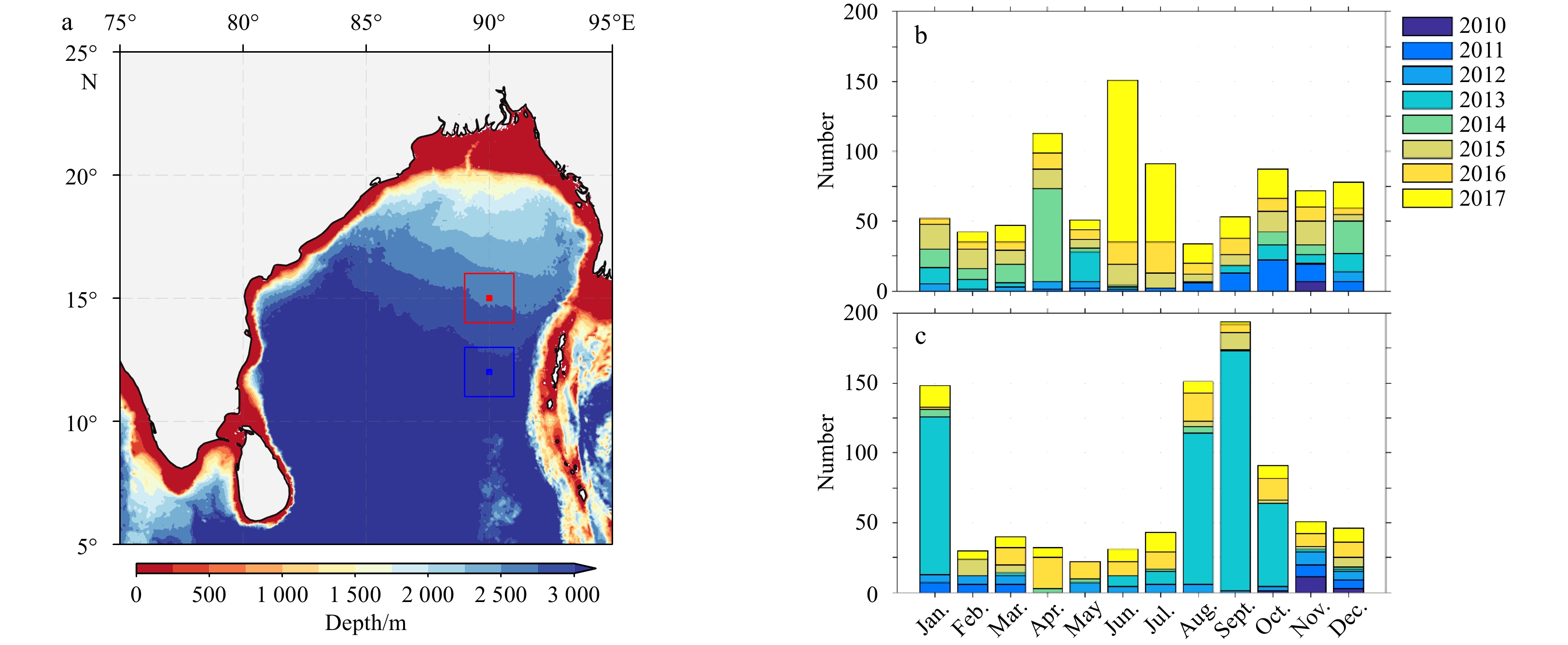
Figure 2. Location of the selected RAMA moorings in the Bay of Bengal (a) and the number of Argo profiles at 15°N, 90°E (area marked with red box) (b), 12°N, 90°E (area marked with blue box) (c) used in the present study.

Figure 3. Comparison of estimated mixed-layer depth (MLD) (a, b) and the barrier-layer thickness (BLT) (c, d) using observations at the RAMA moorings, Argo, HYCOM, and monthly climatology at 15°N, 90°E (a, c) and 12°N, 90°E (b, d). The numbers represent the correlation (r) values between the RAMA estimations with Argo (red), HYCOM (blue), and climatology (green). The standard deviations of the RAMA observations are: ±6.5 (a), ±8.6 (b), ±16 (c), and ±7.4 (d).

Figure 4. Comparison of estimated seasonal cycle of mixed-layer temperature (MLT) (a, b) and mixed-layer salinity (MLS) (c, d) using observations at the RAMA moorings, Argo, HYCOM, and OISST at 15°N, 90°E (a, c) and 12°N, 90°E (b, d). The standard deviations of the RAMA observations are: ±0.9 (a), ±0.7 (b), ±0.2 (c), and ±0.3 (d).

Figure 5. Seasonal cycles of turbulent and radiative heat fluxes (a, b) and mixed-layer heat budget terms (c, d) at 15°N, 90°E (a, c) and 12°N, 90°E (b, d) in the Bay of Bengal. The specific terms and their color notations are given in the legend. The standard deviations of the estimated heat budget terms are:
$\partial T/ \partial t = \pm 0.02,{Q}^{{'}} = \pm 0.06,\mathrm{H}\mathrm{A}\mathrm{d}\mathrm{v} = \pm 0.006,\;\mathrm{a}\mathrm{n}\mathrm{d}\;{Q}_{h} = \pm 0.04$ (c), and$\partial T/ \partial t = \pm 0.02,{Q}^{{'}} = \pm 0.03, $ $ \mathrm{H}\mathrm{A}\mathrm{d}\mathrm{v} = \pm 0.007,\;\mathrm{a}\mathrm{n}\mathrm{d}\;{Q}_{h} = \pm 0.02$ (d).
Figure 6. Seasonal variability of barrier-layer thickness (BLT) and mixed-layer temperature (MLT) (a), mixed-layer
$ \mathrm{H}\mathrm{A}\mathrm{d}\mathrm{v} $ (b), and$ {Q}_{h} $ (c) at 15°N, 90°E (solid lines) and 12°N, 90°E (dashed lines) in the Bay of Bengal. Shaded area represents the ±1σ.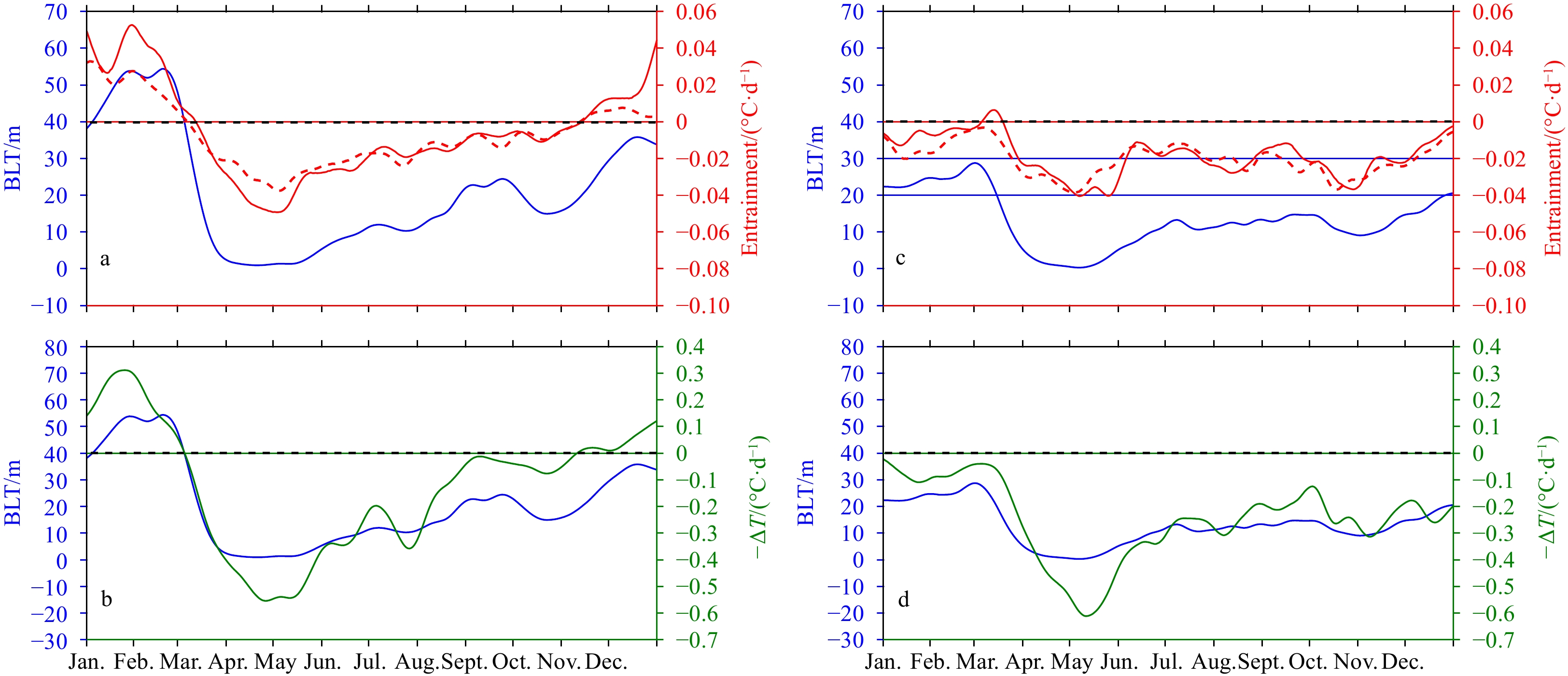
Figure 7. Seasonal variability of barrier-layer thickness (BLT) and entrainment (a, c), and the seasonal variability of BLT and temperature inversion at 15°N, 90°E (a, b) and 12°N, 90°E (c, d) in the BoB. In the upper panels, the red lines represent entrainment estimated considering
${W}_{h} = \mathrm{T}\mathrm{T}\mathrm{D}$ (solid line) and${W}_{h} = \mathrm{D}23$ (dashed line). In the upper (lower) panels, the dahsed lines (black) represent the zero lines for entrainment (temperature inversion). The standard deviation of the estimated parameters are: ±0.02 (red solid) and ±0.01 (red dashed) (a), ±0.23 (green) (b), ±0.01 (red solid) and ±0.008 (red dahsed) (c), and ±0.14 (green) (d).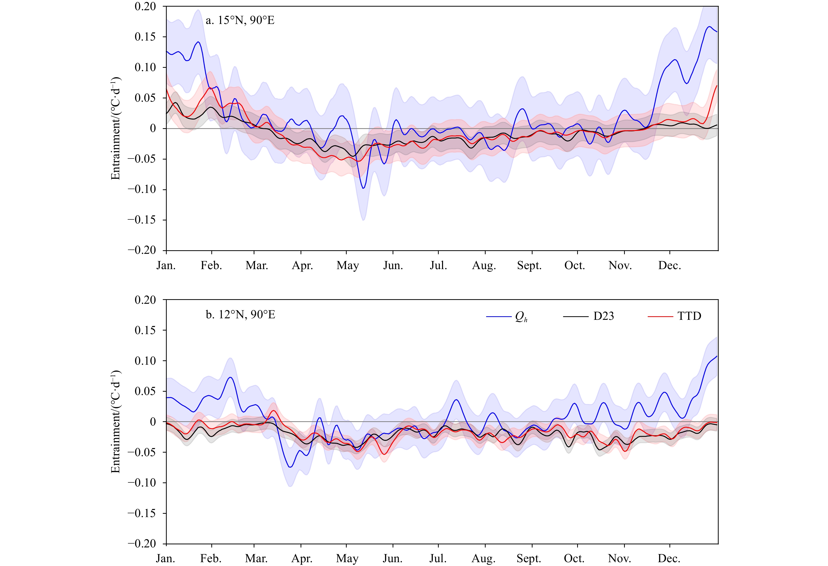
Figure 8. Seasonal variability of
$ {Q}_{h} $ and entrainment,${W}_{h} = \mathrm{T}\mathrm{T}\mathrm{D}$ and${W}_{h} = \mathrm{D}23$ at RAMA stations. Figures represent the average data for 8 years (2010–2017) that have been filtered using a 15-day running mean filter.Table 1. Correlations at the 95% significance level between the estimations from RAMA data and other data sources
Parameter Data source 15°N, 90°E 12°N, 90°E r RMSE r RMSE MLD RAMA-Argo 0.86 [0.58, 0.96] 3.70 0.82 [0.48, 0.94] 8.00 RAMA-HYCOM 0.42 [0.36, 0.52] 7.20 0.90 [0.67, 0.97] 4.00 RAMA-Climatology 0.77 [0.35, 0.93] 11.75 0.80 [0.42, 0.94] 11.80 BLT RAMA-Argo 0.95 [0.85, 0.98] 5.60 0.77 [0.36, 0.93] 4.90 RAMA-HYCOM 0.85 [0.55, 0.95] 12.50 0.95 [0.82, 0.98] 5.00 RAMA-Climatology 0.96 [0.86, 0.98] 5.70 0.88 [0.63, 0.97] 7.40 MLT RAMA-Argo 0.98 [0.95, 0.99] 0.19 0.88 [0.62, 0.97] 0.70 RAMA-HYCOM 0.98 [0.93, 0.99] 0.51 0.92 [0.73, 0.98] 0.62 RAMA-OISST 0.98 [0.97, 0.99] 0.18 0.97 [0.96, 0.98] 0.20 MLS RAMA-Argo 0.81 [0.45, 0.94] 0.23 0.89 [0.65, 0.97] 0.32 RAMA-HYCOM 0.62 [0.08, 0.88] 0.30 0.91 [0.71, 0.97] 0.20 Note: The confidence intervals are noted in square brackets. MLD: mixed-layer depth; BLT: barrier-layer thickness; MLT: mixed-layer temperature; MLS: mixed-layer salinity.  下载: 导出CSV
Table 2. Correlations at the 95% significance level between the estimated barrier-layer thickness (BLT) and several selected parameters at the RAMA moorings
15°N, 90°E 12°N, 90°E BLT-MLT −0.86 [−0.88, −0.83] −0.96 [−0.97, −0.95] BLT-HAdv −0.54 [−0.61, −0.47] −0.11 [−0.21, −0.01] BLT-Qh 0.72 [0.67, 0.77] 0.78 [0.74, 0.82] BLT-(Wh=TTD) 0.98 [0.97, 0.99] 0.88 [0.85, 0.90] BLT-(Wh=D23) 0.97 [0.96, 0.98] 0.79 [0.74, 0.83] BLT-(–ΔT) 0.94 [0.93, 0.95] 0.94 [0.92, 0.96] Note: The confidence intervals are noted in square brackets. MLT: mixed-layer temperature; TTD: top of thermocline depth.
下载: 导出CSV
-
[1] Agarwal N, Sharma R, Parekh A, et al. 2012. Argo observations of barrier layer in the tropical Indian Ocean. Advances in Space Research, 50(5): 642–654. doi: 10.1016/j.asr.2012.05.021 [2] Bosc C, Delcroix T, Maes C. 2009. Barrier layer variability in the western Pacific warm pool from 2000 to 2007. Journal of Geophysical Research, 114(C6): C06023. doi: 10.1029/2008JC005187 [3] Chen Gengxin, Han Weiqing, Li Yuanlong, et al. 2015. Seasonal-to-Interannual time-scale dynamics of the equatorial undercurrent in the Indian Ocean. Journal of Physical Oceanography, 45(6): 1532–1553. doi: 10.1175/jpo-d-14-0225.1 [4] Chowdary J S, Srinivas G, Fousiya T S, et al. 2016. Representation of bay of bengal upper-ocean salinity in general circulation models. Oceanography, 29(2): 38–49. doi: 10.5670/oceanog.2016.37 [5] Cronin M F, McPhaden M J. 2002. Barrier layer formation during westerly wind bursts. Journal of Geophysical Research, 107(C12): 8020. doi: 10.1029/2001JC001171 [6] de Boyer Montegut C, Madec G, Fischer A S, et al. 2004. Mixed layer depth over the global ocean: an examination of profile data and a profile-based climatology. Journal of Geophysical Research, 109(C12): C12003. doi: 10.1029/2004JC002378 [7] de Boyer Montegut C, Vialard J, Shenoi S S C, et al. 2007. Simulated seasonal and interannual variability of the mixed layer heat budget in the northern Indian Ocean. Journal of Climate, 20(13): 3249–3268. doi: 10.1175/JCLI4148.1 [8] Fairall C W, Bradley E F, Hare J E, et al. 2003. Bulk parameterization of air-sea fluxes: updates and verification for the COARE algorithm. Journal of Climate, 16(4): 571–591. doi: 10.1175/1520-0442(2003)016<0571:BPOASF>2.0.CO;2 [9] Felton C S, Subrahmanyam B, Murty V S N, et al. 2014. Estimation of the barrier layer thickness in the Indian Ocean using Aquarius Salinity. Journal of Geophysical Research, 119(7): 4200–4213. doi: 10.1002/2013JC009759 [10] Foltz G R, McPhaden M J. 2009. Impact of barrier layer thickness on SST in the central tropical North Atlantic. Journal of Climate, 22(2): 285–299. doi: 10.1175/2008JCLI2308.1 [11] Girishkumar M S, Ravichandran M, McPhaden M J. 2013. Temperature inversions and their influence on the mixed layer heat budget during the winters of 2006–2007 and 2007–2008 in the Bay of Bengal. Journal of Geophysical Research, 118(5): 2426–2437. doi: 10.1002/jgrc.20192 [12] Girishkumar M S, Ravichandran M, McPhaden M J, et al. 2011. Intraseasonal variability in barrier layer thickness in the south central Bay of Bengal. Journal of Geophysical Research, 116(C3): C03009. doi: 10.1029/2010JC006657 [13] Harenduprakash L, Mitra A K. 1988. Vertical turbulent mass flux below the sea surface and air-sea interaction—monsoon region of the Indian Ocean. Deep-Sea Research Part A. Oceanographic Research Papers, 35(3): 333–346. doi: 10.1016/0198-0149(88)90014-3 [14] Huang Boyin, Thorne P W, Banzon V F, et al. 2017. Extended reconstructed sea surface temperature, version 5 (ERSSTv5): upgrades, validations, and intercomparisons. Journal of Climate, 30(20): 8179–8205. doi: 10.1175/JCLI-D-16-0836.1 [15] Jinadasa S U P, Pathirana G, Ranasinghe P N, et al. 2020. Monsoonal impact on circulation pathways in the Indian Ocean. Acta Oceanologica Sinica, 39(3): 103–112. doi: 10.1007/s13131-020-1557-5 [16] Jouanno J, Marin F, du Penhoat Y, et al. 2011. Seasonal heat balance in the upper 100 m of the equatorial Atlantic Ocean. Journal of Geophysical Research, 116(C9): C09003. doi: 10.1029/2010JC006912 [17] Kumar B P, Vialard J, Lengaigne M, et al. 2012. TropFlux: air-sea fluxes for the global tropical oceans—description and evaluation. Climate Dynamics, 38(7): 1521–1543. doi: 10.1007/s00382-011-1115-0 [18] Lukas R, Lindstrom E. 1991. The mixed layer of the western equatorial Pacific Ocean. Journal of Geophysical Research, 96(S01): 3343–3357. doi: 10.1029/90JC01951 [19] Masumoto Y, Sasaki H, Kagimoto T, et al. 2004. A fifty-year eddy-resolving simulation of the world ocean—Preliminary outcomes of OFES (OGCM for the Earth Simulator). Journal of the Earth Simulator, 1: 35–56 [20] McCreary J P Jr, Kundu P K, Molinari R L. 1993. A numerical investigation of dynamics, thermodynamics and mixed-layer processes in the Indian Ocean. Progress in Oceanography, 31(3): 181–244. doi: 10.1016/0079-6611(93)90002-U [21] McPhaden M J, Foltz G R. 2013. Intraseasonal variations in the surface layer heat balance of the central equatorial Indian Ocean: the importance of zonal advection and vertical mixing. Geophysical Research Letters, 40(11): 2737–2741. doi: 10.1002/grl.50536 [22] McPhaden M J, Meyers G, Ando K, et al. 2009. RAMA: the research moored array for African-Asian-Australian monsoon analysis and prediction. Bulletin of the American Meteorological Society, 90(4): 459–480. doi: 10.1175/2008BAMS2608.1 [23] Narvekar J, Kumar S P. 2006. Seasonal variability of the mixed layer in the central Bay of Bengal and associated changes in nutrients and chlorophyll. Deep-Sea Research Part I: Oceanographic Research Papers, 53(5): 820–835. doi: 10.1016/j.dsr.2006.01.012 [24] Pathirana G, Priyadarshani K. 2020. A mini-warm pool during spring in the Bay of Bengal. Journal of the National Science Foundation of Sri Lanka, 48(4): 345–355. doi: 10.4038/jnsfsr.v48i4.9256 [25] Pathirana G, Priyadarshani K, Wang Dongxiao, et al. 2020. Effect of spring mini-warm pool on the tropical cyclones in the Bay of Bengal: case studies. Journal of Nanjing University of Information Science and Technology (Natural Science Edition), 12(4): 460–471 [26] Rao R R, Sivakumar R. 2000. Seasonal variability of near-surface thermal structure and heat budget of the mixed layer of the tropical Indian Ocean from a new global ocean temperature climatology. Journal of Geophysical Research, 105(C1): 995–1015. doi: 10.1029/1999JC900220 [27] Schott F A, McCreary J P Jr. 2001. The monsoon circulation of the Indian Ocean. Progress in Oceanography, 51(1): 1–123. doi: 10.1016/S0079-6611(01)00083-0 [28] Shee A, Sil S, Gangopadhyay A, et al. 2019. Seasonal evolution of oceanic upper layer processes in the northern Bay of Bengal following a single Argo float. Geophysical Research Letters, 46(10): 5369–5377. doi: 10.1029/2019GL082078 [29] Shenoi S S C, Shankar D, Shetye S R. 2002. Differences in heat budgets of the near-surface Arabian Sea and Bay of Bengal: implications for the summer monsoon. Journal of Geophysical Research, 107(C6): 3052. doi: 10.1029/2000JC000679 [30] Shetye S R, Gouveia A D, Shankar D, et al. 1996. Hydrography and circulation in the western Bay of Bengal during the northeast monsoon. Journal of Geophysical Research, 101(C6): 14011–14025. doi: 10.1029/95JC03307 [31] Sprintall J, Tomczak M. 1992. Evidence of the barrier layer in the surface layer of the tropics. Journal of Geophysical Research, 97(C5): 7305–7316. doi: 10.1029/92JC00407 [32] Thadathil P, Muraleedharan P M, Rao R R, et al. 2007. Observed seasonal variability of barrier layer in the Bay of Bengal. Journal of Geophysical Research, 112(C2): C02009. doi: 10.1029/2006JC003651 [33] Thadathil P, Thoppil P, Rao R R, et al. 2008. Seasonal variability of the observed barrier layer in the Arabian Sea. Journal of Physical Oceanography, 38(3): 624–638. doi: 10.1175/2007JPO3798.1 [34] Vialard J, Delecluse P. 1998a. An OGCM study for the TOGA decade. Part I: role of salinity in the physics of the Western Pacific fresh pool. Journal of Physical Oceanography, 28(6): 1071–1088. doi: 10.1175/1520-0485(1998)028<1071:AOSFTT>2.0.CO;2 [35] Vialard J, Delecluse P. 1998b. An OGCM study for the TOGA decade. Part II: barrier-layer formation and variability. Journal of Physical Oceanography, 28(6): 1089–1106. doi: 10.1175/1520-0485(1998)028<1089:AOSFTT>2.0.CO;2 [36] Vialard J, Foltz G R, McPhaden M J, et al. 2008. Strong Indian Ocean sea surface temperature signals associated with the Madden-Julian Oscillation in late 2007 and early 2008. Geophysical Research Letters, 35(19): L19608. doi: 10.1029/2008GL035238 [37] Vinayachandran P N, Murty V S N, Babu V R. 2002. Observations of barrier layer formation in the Bay of Bengal during summer monsoon. Journal of Geophysical Research, 107(C12): 8018. doi: 10.1029/2001JC000831 [38] Warner S J, Becherer J, Pujiana K, et al. 2016. Monsoon mixing cycles in the Bay of Bengal: a year-long subsurface mixing record. Oceanography, 29(2): 158–169. doi: 10.5670/oceanog.2016.48 期刊类型引用(1)
1. Wenshu Lin, Yun Qiu, Xutao Ni, et al. Evolution characteristics and mechanisms of the spring warm pool in the Bay of Bengal. Frontiers in Marine Science, 2024, 11  必应学术
必应学术其他类型引用(0)
-


 DownLoad:


 必应学术
必应学术 点击查看大图
计量
- 文章访问数: 1265
- HTML全文浏览量: 470
- PDF下载量: 95
- 被引次数: 1
目录
1. Introduction
2. Data and methods
2.1 Mixed-layer depth and barrier-layer thickness
2.2 Mixed-layer heat budget
2.3 Entrainment and vertical velocity
3. Results and discussion
3.1 Seasonal MLD and BLT at the RAMA moorings
3.2 Seasonal MLT and MLS at the RAMA moorings
3.3 Seasonal mixed-layer heat budget at the RAMA moorings
3.4 Effect of seasonal BLT on
$ \boldsymbol{M}\boldsymbol{L}\boldsymbol{T} $ ,$ \boldsymbol{H}\boldsymbol{A}\boldsymbol{d}\boldsymbol{v} $ and${{{\boldsymbol{Q}}}}_{{{\boldsymbol{h}}}}$ 3.5 Effect of seasonal BLT on entrainment and temperature inversion
4. Summary
Acknowledgements


