

Tropical cyclone genesis over the western North Pacific simulated by Coupled Model Intercomparison Project Phase 6 models
-
Abstract: Threatening millions of people and causing billions of dollars in losses, tropical cyclones (TCs) are among the most severe natural hazards in the world, especially over the western North Pacific. However, the response of TCs to a warming or changing climate has been the subject of considerable research, often with conflicting results. In this study, the abilities of Coupled Model Intercomparison Project (CMIP) Phase 6 (CMIP6) models to simulate TC genesis are assessed through historical simulations. The results indicate that a systematic humidity bias persists in most CMIP6 models from corresponding CMIP Phase 5 models, which leads to an overestimation of climatological TC genesis. However, the annual cycle of TC genesis is well captured by CMIP6 models. The abilities of 25 models to simulate the geographical patterns of TC genesis vary significantly. In addition, seven models are identified as well simulated models, but seven models are identified as poorly simulated ones. A comparison of the environmental variables for TC genesis in the well-simulated group and the poorly simulated group identifies moisture in the mid-troposphere as a key factor in the realistic simulation of El Niño-Southern Oscillation (ENSO) impacts on TC genesis. In contrast with the observations, the poorly simulated group does not reproduce the suppressing effect of negative moisture anomalies on TC genesis in the northwestern region (20°–30°N, 120°–145°E) during El Niño years. Given the interaction between TC and ENSO, these results provide a guidance for future TC projections under climate change by CMIP6 models.
-
Key words:
- CMIP6 /
- tropical cyclone /
- genesis potential index /
- relative humidity
-
1. Introduction
Tropical cyclones (TCs) are a major natural disaster that causes large casualties and extensive socioeconomic damage every year (Shultz et al., 2005). The western North Pacific (WNP) experiences the most TCs, accounting for almost one third of global TCs. TCs over the WNP exhibit significant variabilities in both frequency and intensity (Klotzbach, 2014; Liu and Chan, 2008; Maloney and Hartmann, 2001; Wang and Chan, 2002; Wang and Liu, 2016). They are subject to multi-scale climate phenomena, such as the Madden-Julian Oscillation (Li and Zhou, 2013), El Niño-Southern Oscillation (ENSO; Chia and Ropelewski, 2002; Wu et al., 2021), and Pacific Decadal Oscillation (Aiyyer and Thorncroft, 2011; Wang et al., 2010). Hence, future projections of TCs continue to be challenged (Knutson et al., 2010).
As the dominant source of interannual variability, ENSO has a pronounced influence on weather and climate variations worldwide (McPhaden et al., 2006). As ENSO can effectively change large-scale atmospheric circulations and oceanic processes, it can also significantly modulate global TC activities (Aiyyer and Thorncroft, 2011; Chan, 1985; Wang et al., 2010). For example, during El Niño years, TCs tend to form closer to the international dateline (Bell et al., 2014). Therefore, ENSO-associated TC teleconnections are essential for the seasonal forecasting of TCs and long-term TC projections under climate change (Mori et al., 2013). Further, the ability of current climate models to simulate the connections between TCs and ENSO should be evaluated.
Previous studies have suggested that TC genesis location can affect the metrics of TCs, such as track, intensity, and duration (Chan and Liu, 2004; Lin and Chan, 2015; Yonekura and Hall, 2011, 2014). Despite the lack of a quantitative theory, empirical indices have been developed to quantify TC genesis numbers (TCGNs) based on the large-scale environment (Emanuel and Nolan, 2004; Gray, 1979; Watterson et al., 1995). Estimates of long-term TC genesis variations in global models are commonly achieved using three methods: (1) direct simulation, (2) dynamical downscaling, and (3) genesis indices (Emanuel, 2013). The direct simulation is sensitive to horizontal resolutions, reproduces much lower TC frequencies, and leads to significant deficiencies in the geographical patterns of TC formation in Coupled Model Intercomparison Project (CMIP) Phase 5 (CMIP5; Camargo, 2013). A climate model with a low horizontal resolution do not has the ability to reproduce TC genesis (Camargo et al., 2014). Dynamical downscaling is able to reconstruct local TCs. However, it suffers from a mismatch between regional models and global models and a lack of feedbacks to the global system (Knutson et al., 2008). Conversely, genesis indices have a strong empirical foundation and account for both global climate variabilities and feedbacks. Thus, they can effectively reproduce TC genesis, given TC intensity and track are not considered (Emanuel, 2013).
As an international endeavor to understand future climate changes, the CMIP Phase 6 (CMIP6) provides state-of-art global models to project TC activities under climate change over the WNP. However, the reliability of the large-scale environment for TC genesis in each coupled model should be evaluated prior to projection, especially considering the considerable bias in climate models such as CMIP5 (Knutson et al., 2013). Moreover, Camargo et al. (2007b) reported an overestimation of the simulated genesis potential index in five atmospheric climate models. Previous studies have indicated that CMIP Phase 3 (CMIP3) and CMIP5 models typically produce higher relative humidity, an important factor for TC genesis, when compared to observations (Song et al., 2015; Walsh et al., 2013). Furthermore, with respect to the spatial patterns of TC genesis, Shen et al. (2020) discovered an eastward bias in TC genesis locations in downscaling experiments using the Community Atmosphere Model (version 5) of CMIP5 datasets. Considering significant improvements in resolution and parametrization from CMIP5 to CMIP6 (Eyring et al., 2016), it is essential to assess the CMIP6 model performances in reproducing TC genesis over the WNP.
The remainder of this paper is organized as follows. Section 2 introduces the observation, reanalysis datasets, CMIP6 models and methods including the genesis potential index (GPI) used in this study. Section 3 examines simulations of TC genesis based on the GPI. Section 4 evaluates and interprets the TC genesis simulation performance of 25 CMIP6 models. Finally, the discussion and conclusions are presented in Section 5.
2. Data and methods
2.1 Observations and reanalysis products
TC best-track historical data are obtained from the International Best Track Archive for Climate Stewardship (IBTrACS) Project, version 4 (Knapp et al., 2010). The dataset combines information from numerous TC datasets, such as TC locations and maximum sustained wind speeds from the U.S. Joint Typhoon Warning Center and Hong Kong Observatory. In this study, TCs are excluded if their maximum sustained wind speed never reaches 34 kn (1 kn=1.852 km/h) in their entire life cycle owing to the high uncertainty in detecting weak tropical depressions (Klotzbach and Landsea, 2015). A system is defined as a TC when its maximum sustained wind speed reaches 34 kn for the first time.
The National Center for Environmental Prediction/National Center for Atmospheric Research (NCEP/NCAR) reanalysis (Kalnay et al., 1996) is used to analyze large-scale circulation. NCEP/NCAR reanalysis has been extensively used to construct and assess the GPI (Camargo et al., 2007a, b, 2009). The monthly mean NCEP/NCAR reanalysis provides global coverage of meteorological variables from the surface to 10 hPa, with a horizontal resolution of 2.5° × 2.5° (latitude × longitude). The variables used in this study include air temperature, specific humidity, relative humidity, wind speed, and sea level pressure. Monthly sea surface temperatures (SSTs) are obtained from the National Oceanic and Atmospheric Administration Extended Reconstruction SST (ERSST), version 5 (ERSSTv5; Huang et al., 2017). The ERSSTv5 dataset is based on statistical interpolation of data from the International Comprehensive Ocean-Atmosphere Data Set release 3.0 Argo float data, as well as estimates of sea ice coverage from the Hadley Centre Sea Ice and Sea Surface Temperature dataset. ERSSTv5 affords global coverage from 1854 with a horizontal resolution of 2°. European Centre for Medium-Range Weather Forecasts ERA5 (Hersbach et al., 2020) data are also used to verify the robustness of the results. As the results derived using ERA5 are similar to those using NCEP/NCAR reanalysis, they are not explicitly presented in this study.
2.2 CMIP6 models
GPIs calculated using CMIP6 historical simulations (Eyring et al., 2016) are examined in this study. The protocol for the historical simulations (experiment name: “historical”) calls for 165-year simulations (from 1850 to 2014), with forcing based on observations whenever possible (Hoesly et al., 2018; Meinshausen et al., 2017). Outputs from 25 different Atmosphere-Ocean General Circulation Models are evaluated (Table 1). Information about their host centers and horizontal resolutions are listed in Table 2. Different models have different horizontal resolutions. Therefore, to facilitate inter-comparisons between different models, all outputs are bilinearly interpolated to a regular grid with a horizontal resolution of 1° × 1° (latitude × longitude). The common period for observations, reanalysis, and CMIP6 outputs is 1980–2014. Thus, we focus on the performance of GPIs simulated by CMIP6 during this 35-year period.
Table 1. List of the 25 CMIP6 models employed in this studyNo. Model Institute ID Resolution (number of grids, lon×lat) Atmosphere Ocean 1 ACCESS-CM2 CSIRO-ARCCSS 192×144 360×300 2 ACCESS-ESM1-5 CSIRO 192×145 360×300 3 BCC-CSM2-MR BCC 320×160 360×232 4 BCC-ESM1 BCC 128×64 360×232 5 CAMS-CSM1-0 CAMS 320×160 360×200 6 CanESM5 CCCma 128×64 361×290 7 CAS-ESM2-0 CAS 256×128 362×196 8 CESM2 NCAR 288×192 320×384 9 CESM2-FV2 NCAR 144×96 320×384 10 CESM2-WACCM NCAR 288×192 320×384 11 CESM2-WACCM-FV2 NCAR 144×96 320×384 12 CMCC-CM2-SR5 CMCC 288×192 362×292 13 FGOALS-g3 CAS 180×80 360×218 14 FIO-ESM-2-0 FIO-QLNM 192×288 320×384 15 GISS-E2-1-G NASA-GISS 144×90 360×180 16 GISS-E2-1-H NASA-GISS 144×90 360×180 17 MCM-UA-1-0 UA 96×80 192×80 18 MIROC6 MIROC 256×128 360×256 19 MPI-ESM1-2-HR MPI-M DWD DKRZ 384×192 802×404 20 MRI-ESM2-0 MRI 320×160 360×364 21 NESM3 NUIST 192×96 384×362 22 NorESM2-LM NCC 144×96 360×384 23 NorESM2-MM NCC 288×192 360×384 24 SAM0-UNICON SNU 288×192 320×384 25 TaiESM1 AS-RCEC 288×192 320×384 Note: CSIRO-ARCCSS: Commonwealth Scientific and Industrial Research Organisation-Australian Research Council Centre of Excellence for Climate System Science; CSIRO: Commonwealth Scientific and Industrial Research Organisation; BCC: Beijing Climate Center; CAMS: Chinese Academy of Meteorological Sciences; CCCma: Canadian Centre for Climate Modelling and Analysis; CAS: Chinese Academy of Sciences; NCAR: National Center for Atmospheric Research; CMCC: Fondazione Centro Euro-Mediterraneo sui Cambiamenti Climatici; FIO-QLNM: First Institute of Oceanography-Ministry of Natural Resources, Qingdao National Laboratory for Marine Science and Technology; NASA-GISS: National Aeronautics and Space Administration-Goddard Institute for Space Studies; UA: University of Arizona-Department of Geosciences; MIROC: Japan Agency for Marine-Earth Science and Technology, Atmosphere and Ocean Research Institute, National Institute for Environmental Studies, RIKEN Center for Computational Science; MPI-M DWD DKRZ: Max Planck Institute for Meteorology, German Meteorological Service, German Climate Computing Center; MRI: Meteorological Research Institute; NUIST: Nanjing University of Information Science and Technology; NCC: Norwegian Climate Centre; SNU: Seoul National University; AS-RCEC: Academia Sinica-Research Center for Environmental Changes. | Show Table DownLoad:
CSV
Table 2. Centered pattern correlation coefficients (CPCCs) of 25 CMIP6 models with the observed GPIs
DownLoad:
CSV
Table 2. Centered pattern correlation coefficients (CPCCs) of 25 CMIP6 models with the observed GPIsEvaluation Model CPCC Well-simulated TaiESM1 0.94 ACCESS-CM2 0.93 FIO-ESM-2-0 0.89 BCC-CSM2-MR 0.88 CESM2-WACCM 0.86 CMCC-CM2-SR5 0.85 NorESM2-LM 0.85 Moderately simulated CESM2 0.83 BCC-ESM1 0.83 CAMS-CSM1-0 0.82 FGOALS-g3 0.81 NorESM2-MM 0.80 SAM0-UNICON 0.79 CESM2-WACCM-FV2 0.79 CESM2-FV2 0.77 ACCESS-ESM1-5 0.77 MIROC6 0.75 CAS-ESM2-0 0.72 Poorly simulated MRI-ESM2-0 0.71 MPI-ESM1-2-HR 0.71 GISS-E2-1-H 0.70 GISS-E2-1-G 0.69 CanESM5 0.65 MCM-UA-1-0 0.51 NESM3 0.48 Note: All CPCCs depict statistical significance based on a two-tailed Student’s t-test (>99%). | Show TableDownLoad:
CSV
2.3 Definitions of El Niño and La Niña years
El Niño and La Niña years are defined based on the Niño 3.4 index (i.e., mean SST anomalies within 5°N–5°S and 170°–120°W). The following analyses focus on the TC season (July–October) over the WNP. Years when the mean Niño 3.4 index during TC season is higher (lower) than 1°C are defined as El Niño (La Niña) years. Hence, during the period of 1980–2014, four El Niño years (i.e., 1982, 1987, 1997, and 2002) and four La Niña years (i.e., 1988, 1998, 1999, and 2010) are identified. The same procedures are performed for each of the 25 CMIP6 models so that El Niño and La Niña years defined for each model coordinate with the outputs of that model.
2.4 Methods
The GPI adopted in this study was developed by Emanuel and Nolan (2004) and has been widely used (Bruyère et al., 2012; Camargo et al., 2007a, b; Fu et al., 2017; Gao et al., 2020; Yan et al., 2019). The GPI is defined as follows:
$$ {\rm{GPI}}={\left|{10}^{5}{\eta }_{850}\right|}^{3/2}{\left(\frac{{H}_{600}}{50}\right)}^{3}{\left(\frac{{V}_{{\rm{pot}}}}{70}\right)}^{3}{\left(1+0.1{V}_{{\rm{shear}}}\right)}^{-2}, $$ (1) where
$ {\mathrm{\eta }}_{850} $ is the absolute vorticity at 850 hPa,$ {H}_{600} $ is the relative humidity at 600 hPa,$ {V}_{\mathrm{p}\mathrm{o}\mathrm{t}} $ is the potential intensity, and$ {V}_{\mathrm{s}\mathrm{h}\mathrm{e}\mathrm{a}\mathrm{r}} $ is the magnitude of vertical wind shear between 850 hPa and 200 hPa. Further,$ {V}_{\mathrm{p}\mathrm{o}\mathrm{t}} $ is calculated as follows (Bister and Emanuel, 1998; Gilford et al., 2017):$$ {V}_{{\rm{pot}}}^{2}=\frac{{C}_{{\rm{K}}}}{{C}_{{\rm{D}}}}\frac{\left({T}_{{\rm{s}}}-{T}_{{\rm{o}}}\right)}{{T}_{{\rm{o}}}}\left({h}_{{\rm{o}}}^{*}-{h}^{*}\right),$$ (2) where
$ {C}_{\mathrm{K}} $ and$ {C}_{\mathrm{D}} $ are the enthalpy and momentum surface exchange coefficients, respectively;$ {T}_{\mathrm{s}} $ is the SST;$ {T}_{\mathrm{o}} $ is the outflow temperature at the level of neutral buoyancy for a saturated air parcel lifted from sea level;$ {h}_{\mathrm{o}}^{\mathrm{*}} $ is the saturation moist static energy at the sea surface; and$ {h}^{\mathrm{*}} $ is the saturation moist static energy of the air above the boundary layer. The ratio of$ {C}_{\mathrm{K}} $ to$ {C}_{\mathrm{D}} $ depends on the sea state. The one standard deviation of this ratio is from 0.17 to 1.05, based on the energy and momentum budget analysis using data from the Coupled Boundary Layers Air-Sea Transfer field program in 2003. In this study, it is set to 0.9 according to previous studies (Gilford et al., 2017; Wang et al., 2014; Wing et al., 2015).The centered pattern correlation coefficients (CPCCs, also known as anomaly correlation coefficients) are calculated between simulations and observations for each CMIP6 model. Corresponding p-values are given by the two-tailed Student’s t-test. In addition, the Hotelling’s T-squared test (Hotelling, 1940) and the Steiger’s Z-test (Steiger, 1980) are applied to test the statistical significance of the difference between two correlation coefficients. The Hotelling’s T-squared statistic, which obeys the Hotelling’s T-squared distribution, is defined as follows:
$$ {T}^{2}=\left({r}_{12}-{r}_{13}\right)\sqrt{\frac{\left(n-3\right)\left(1+{r}_{23}\right)}{2\left|D\right|}}, $$ (3) where n is the number of records. The degree of freedom is n−3. D is calculated using Eq. (4):
$$ \begin{array}{c}D=1+2{r}_{12}{r}_{13}{r}_{23}-{r}_{12}^{2}-{r}_{13}^{2}-{r}_{23}^{2},\end{array} $$ (4) where
$ {r}_{12} $ and$ {r}_{13} $ are the correlations between the GPIs in two models (denoted with subscripts 2 and 3, respectively) with the GPI from observations (denoted with subscript 1); and$ {r}_{23} $ is the correlation of the GPIs between the two models. The Steiger’s Z-test, which assumes a standard normal distribution, is defined as follows:$$ Z=\left({K}_{12}-{K}_{13}\right)\sqrt{\dfrac{\left(n-3\right)}{2-2c}},$$ (5) where
$ {K}_{12} $ and$ {K}_{13} $ are the transformed correlations from$ {r}_{12} $ and$ {r}_{13} $ , based on$$ K=\frac{1}{2}\left[\ln\left(1+r\right)-\ln\left(1-r\right)\right], $$ (6) and c is defined as
$$ c=\dfrac{{r}_{23}\left(1-2{\bar{r}}^{2}\right)-\dfrac{1}{2}{\bar{r}}^{2}\left(1-2{\bar{r}}^{2}-{r}_{23}^{2}\right)}{{\left(1-{\bar{r}}^{2}\right)}^{2}}, $$ (7) where
$$\bar{r}=\frac{{r}_{12}+{r}_{13}}{2}. $$ (8) The contribution of a variable to GPI in Eq. (1) is evaluated using the method proposed by Camargo et al. (2007a). Taking
$ {H}_{600} $ as an example, the contribution of$ {H}_{600} $ is calculated as follows:$$ \begin{array}{c}{\Delta {\rm{GPI}}}_{{H}_{600}}={\rm{GPI}}\left({H}_{600-{\rm{EL}}}\right)-{\rm{GPI}}\left({H}_{600-{\rm{LA}}}\right),\end{array} $$ (9) where
${\Delta {\rm{GPI}}}_{{{H}}_{600}}$ is the difference in the contribution of$ {H}_{600} $ to the GPI between El Niño and La Niña years;${\rm{GPI}}\left({H}_{600-\mathrm{E}\mathrm{L}}\right)$ is the GPI computed using climatological data, where$ {H}_{600} $ is for El Niño years; and${\rm{GPI}}\left({H}_{600-\mathrm{L}\mathrm{a}}\right)$ is the same as${\rm{GPI}}\left({H}_{600-\mathrm{E}\mathrm{L}}\right)$ , except that$ {H}_{600} $ is obtained in La Niña years.CPCC is a useful measure of the simulation skill, especially regarding the spatial patterns. However, it is not sensitive to systematic biases. This problem can be solved by considering an algebraic manipulation of the mean squared error (Murphy, 1988). Therefore, we employ a skill score, which reflects the percentage improvement over the reference simulation (also known as the climatology simulation), defined as follows:
$$ {\rm{skill}}\_{\rm{score}}=1-\frac{{{\rm{MSE}}}_{\mathrm{s}}}{{{\rm{MSE}}}_{\mathrm{r}\mathrm{e}\mathrm{f}}}, $$ (10) where
${{\rm{MSE}}}_{\mathrm{s}}$ and${{\rm{MSE}}}_{\mathrm{r}\mathrm{e}\mathrm{f}}$ are the mean squared error of the simulated and reference simulations, respectively. The skill score ranges from negative infinity to 1. A negative value indicates that the simulation is less accurate than the reference simulation.3. Observed TC genesis and GPI
All TC genesis locations in IBTrACS from 1980–2014 are marked with black dots in Fig. 1a. The observed TCGNs are binned to a regular grid of 2.5° × 2.5° (latitude × longitude) and the distributions of cumulative TCGNs are shown in Fig. 1a with colored squares. The GPIs in Eq. (1) calculated from NCEP/NCAR reanalysis and ERSSTv5 data are shown in Fig. 1b, which demonstrates a good agreement with IBTrACS. The CPCC between the colors in Figs 1a and b is 0.77, which is statistically significant at a 99% confidence level. This pattern is also consistent with many previous studies (Huang et al., 2011; Li and Wang, 2014). However, some discrepancy in the spatial distribution is discernible. For example, the GPI in Fig. 1b is more homogeneous than the TCGN in Fig. 1a. The spatial variability can be measured using standard deviation within a domain, i.e.,
$ \dfrac{1}{N}\displaystyle\sum _{i,j\in S}{\left({X}_{ij}-\stackrel{-}{X}\right)}^{2} $ . Here, S denotes the domain in Figs 1a and b, N is the number of grid points within domain S, X is a dummy variable denoting TCGN for Fig. 1a and GPI for Fig. 1b,$ \stackrel{-}{X} $ is the mean X within domain S, and i and j are the horizontal and meridional index within domain S. The spatial variability of the observations is 3.1, whereas the spatial variability of the GPI is only 1.6. Nevertheless, a large portion of the difference in spatial variability is attributable to the fact that the TCGNs are natural numbers, whereas GPI are rational numbers (Tippett et al., 2011). Figure 1. The observed and simulated climatological TC genesis during the period of 1980–2014 over the WNP. a. Results from IBTrACS. Black dots indicate TC genesis locations and colors represent TCGN in a regular grid with a horizontal resolution of 2.5°×2.5° (longitude×latitude). b. GPI derived using ERSSTv5 and NCEP/NCAR reanalysis. R represents the CPCC between the observation and simulation, which passes the two-tailed Student’s t-test at p = 0.01.
The annual cycles of TCGN and GPI are compared in Fig. 2. The GPI captures both the active TC genesis from July to October and the reduced TC genesis from January to April. The correlation coefficient between TCGN and GPI in Fig. 2 is 0.96, which is significant at a confidence level of 99%. The maximum GPI coincides with the observed TCGN in August, although the maximum GPI is less than the maximum observation by approximately 20%. Furthermore, the standard deviation of the annual GPI is 6, which is half that of the observations (standard deviation of 12). This is attributed to overestimation of TC genesis during unfavorable seasons and underestimation during favorable seasons. Menkes et al. (2012) also found that the seasonal variation of other GPIs is weaker than the observation.
 Figure 2. The observed and simulated annual cycle of TCGN in the period of 1980–2014 over the WNP. Red line represents the results from IBTrACS, and blue line represents the GPI derived using ERSSTv5 and NCEP/NCAR reanalysis. R is the Pearson linear correlation coefficient, which passes the two-tailed Student’s t-test at p = 0.01.
It has been long recognized that TC activities have a strong interannual variability in all ocean basins (Landsea, 2000), with vast research efforts revealing that ENSO, the leading source of interannual variabilities, can modulate TCs in the WNP (Chan, 1985; Chia and Ropelewski, 2002; Du et al., 2011; Wang and Chan, 2002; Wang et al., 1999, 2013; Wang and Wang, 2013; Yang et al., 2018a). To analyze the observed relationship between TC genesis and ENSO over the WNP, we divided the WNP into four regions following the definition in Wang and Chan (2002): northwest quadrant (NW, 20°–30°N, 120°–145°E), northeast quadrant (NE, 20°–30°N, 145°–180°E), southeast quadrant (SE, 0°–20°N, 145°–180°E), and southwest quadrant (SW, 0°–20°N, 120°–145°E). During El Niño years, TCs are more likely to occur in the SE, with a statistically significant decrease in the NW (Fig. 3a). In the SE, there are as many as 29 TCs in four El Niño years but only two TCs in four La Niña years. Contrary to SE, only two TCs are found in four El Niño years with 18 TCs in four La Niña years in the NW. As illustrated in Fig. 3b, the GPI exhibits positive anomalies in the SE and negative anomalies in the NW during El Niño years. Note that the magnitude of positive anomalies is significantly greater than the negative anomalies, which is consistent with the IBTrACS observations. The decrease of TCGN in the NW with an increase in the SE during El Niño years leads to no noticeable ENSO’s impact on the total TCG but a pronounced southeastward shift in TC formation location. Figure 4 shows the cumulative distribution of TC genesis longitude and latitude for El Niño and La Niña years. An eastward shift of TC genesis by 8°–10° longitude and a southward shift of TC genesis by 4°–5° latitude are detected in both the IBTrACS and the GPI. The southeastward shift in TC genesis during El Niño years is attributable to the increased low-level vorticity and reduced vertical wind shear in the SE, as well as an expanded monsoon trough (Wang and Chan, 2002). Notably, the profound eastward shift of TC genesis leads to more intense and long-lived TCs during El Niño years (Camargo and Sobel, 2005). Overall, the GPI in Eq. (1) captures the main characteristics of TC genesis at climatological, interannual, and annual timescales.
 Figure 3. TC genesis during El Niño and La Niña years over the WNP. a. Results from IBTrACS. Red dots and blue dots indicate TC genesis locations in El Niño and La Niña years, respectively. b. Difference in the GPI (derived using ERSSTv5 and NCEP/NCAR reanalysis) between El Niño and La Niña years. Shaded areas represent the 99% confidence level according to the two-tailed Student’s t-test. Zonal gray line at 20°N and meridional line at 145°E divide the WNP into four subregions.
 Figure 4. Cumulative distribution function of the longitude (a) and latitude (b) of TC genesis locations over the WNP. Blue and red lines represent the results of La Niña (LN) and El Niño (EN) years, respectively. The observed TC genesis is shown in solid lines and the observed GPIs (derived using ERSSTv5 and NCEP/NCAR reanalysis) are shown in dashed lines.
4. Evaluation of TC genesis in CMIP6 models
4.1 Climatology and annual cycle of TC genesis in CMIP6 models
Figure 5 illustrates the GPI simulated in 25 CMIP6 models (Figs 5b-z) and their multi-model ensemble (MME, Fig. 5a). The GPI obtained with ERSSTv5 and NCEP/NCAR reanalysis is shown in Fig. 6, which is hereinafter referred to as the observed GPI, although the NCEP/NCAR reanalysis products are not observations. The common eastward extension of the TC genesis bias over the WNP compared with the observations is observed in all CMIP6 models. Such bias has previously been reported using other models (Camargo et al., 2005; Shen et al., 2020; Yokoi et al., 2009). Shen et al. (2020) ascribed the eastward bias to overestimated humidity in the eastern region of the WNP. Meanwhile, the TCGN over the WNP is greatly overestimated in all models except ACCESS-EMM1-5 (Fig. 5c), BCC-CSM2-MR (Fig. 5d), CanESM5 (Fig. 5g), MCM-UA-1-0 (Fig. 5r), and SAM0-UNICON (Fig. 5y). A positive GPI systematic bias also exists in most CMIP5 models (Song et al., 2015). Based on a qualitive comparison with the results in Song et al. (2015), the climatological overestimation of TCGN persists in CMIP5/6 models. The overestimation in GPI is mainly attributable to the positive bias in relative humidity in the mid-troposphere. The impact of positive bias in relative humidity on the GPI is illustrated in Fig. 7. The aforementioned five models (i.e., ACCESS-EMM1-5, BCC-CSM2-MR, CanESM5, MCM-UA-1-0, and SAM0-UNICON) without the systematic bias effectively reproduce the relative humidity in the mid-troposphere. In contrast, the other 20 CMIP6 models exhibit substantial overestimations of relative humidity in the mid-troposphere. Tian et al. (2013) argued that an overestimation of relative humidity led to a higher GPI than reanalysis in LASG/IAP AGCM. Biases of moisture are also found in four CMIP5 models, mainly caused by the overestimation of the frequency of vertical velocity at 500 hPa occurrence (Yang et al., 2018b). The MME of the 25 CMIP6 models also exhibits an eastward extension for TC genesis and higher GPI due to the systematic humidity bias (Figs 5a and 7a). After performing normalization via subtracting the corresponding climatological mean and being divided by the standard deviation, the GPIs simulated by all 25 CMIP6 models (Fig. 8) relatively effectively reconstruct the annual cycle of TCGN shown in Fig. 2. Although the maximum normalized GPI of GISS-E2-1-G (1.95), MIROC6 (1.93), CanESM5 (1.92), GISS-E2-1-H (1.87), MRI-ESM2-0 (1.85) and NorESM2-LM (1.84) is significantly higher than that of the observation (1.62), the systematic humidity bias results in an overestimation of climatological GPI but has a trivial impact on the annual cycle.
 Figure 5. The simulated climatological GPIs over the WNP in CMIP6 models. a. Multi-model ensemble (MME) of 25 CMIP6 models and b–z. simulations in each of 25 CMIP6 models. The skill score of each model is shown on the upper-right corner from a to z.
 Figure 6. The GPI obtained with ERSSTv5 and NCEP/NCAR reanalysis.
 Figure 7. The impacts of the
$ {H}_{600} $ bias on the GPI. a. Ensemble mean impact of 25 CMIP6 models and b–z. impacts for each of 25 CMIP6 models. The impacts shown by shaded areas is statistically significant at the 99% confidence level. Figure 8. Annual cycle of the observed GPI (thick black line) and the simulated GPIs in 25 CMIP6 models. All GPIs are normalized by subtracting the corresponding climatological mean and dividing by the standard deviation. Numbers in the legend are the serial numbers corresponding to the 25 CMIP6 models in Table 1.
The multi-model mean is generally superior to a single model because random errors tend to cancel each other out in the multi-model mean, and this value tends to exhibit greater consistency and reliability than individual members (Hagedorn et al., 2005). However, the skill score of MME is −0.78, which is smaller than that of ACCESS-EMM1-5 (−0.51). The fact that the MME does not outperform some individual models (i.e., ACCESS-EMM1-5) may be ascribed to the systematic moisture bias in most CMIP6 models.
The ability to simulate the spatial pattern of climatological TC genesis is examined using the CPCCs between the simulated GPIs in each CMIP6 model and the observed GPI (Table 2). The two-tailed Student’s t-test is applied to test the significance of the CPCCs. The 25 CMIP6 models exhibit variable simulation performance regarding TC genesis locations. The reasons for different model performances can be detected by grouping the models into a well-simulated group and a poorly simulated group. The CPCCs of all models are then sorted from high to low. The first (last) 25th percentile is categorized as the well-simulated (poorly simulated) group, resulting in seven models in the well-simulated group (i.e., ACCESS-CM2, BCC-CSM2-MR, CESM2-WACCM, CMCC-CM2-SR5, FIO-ESM-2-0, NorESM2-LM, and TaiESM1) and seven models in the poorly simulated group (i.e., MRI-ESM2-0, MRI-ESM1-2-HR, CanESM5, GISS-E2-1-G, GISS-E2-1-H, MCM-UA-1-0, and NESM3). The MME of the well-simulated (poorly simulated) group is referred to as WMME (PMME) hereinafter. The WMME has a CPCC of 0.93 with the observed GPI, which is higher than that of MME. In contrast, the PMME has a CPCC of 0.72 with the observed GPI. The difference between the CPCCs of WMME and PMME (Table 3) is statistically significant according to both the Hotelling’s T-squared test and the Steiger’s Z-test (two-tailed, p<0.01).
Table 3. R2 difference among CPCCs of WMME, MME, and PMME.WMME MME PMME WMME (0.93) 0 0.03 0.35 MME (0.91) −0.03 0 0.31 PMME (0.72) −0.35 −0.31 0 Note: Values in bold font were applied to statistically significant differences (two-tailed, p<0.01) based on the Hotelling’s T-squared test and Steiger’s Z-test. | Show TableDownLoad:
CSV
4.2 Interannual variability of TC genesis in WMME and PMME
ENSO plays an important role in modulating WNP TC genesis due to the change in the upward branch of Walker circulation (Tan et al., 2019) and the propagation of wave train responding to SST anomalies (Chen et al., 1998). The correlation between ENSO index (i.e., Niño 3.4) is not significant while the TC genesis location are profoundly modified by ENSO signal, which reveals that the skill to simulating spatial pattern is the leading role in reproducing ENSO’s impact on TC genesis. Therefore, simulated ENSO’s impact on TC genesis in CMIP6 models are examined by comparing the well-simulated and poorly simulated groups. Figure 9 illustrates the differences in the GPI between El Niño and La Niña years in the two groups. The well-simulated group (Fig. 9a) resembles the observed GPI (contours in Fig. 9). Moreover, positive anomalies in the SE and the negative anomalies in the SW and NW are captured. Given that climate models, such as CMIP3 and CMIP5 models (Bellenger et al., 2014; Wengel et al., 2018), tend to yield a large variance of ENSO amplitudes, the ENSO’s impacts on TCs also vary from model to model. The mean Niño 3.4 for TC season in WMME ranges from −3 to 3, whereas that in ERSSTv5 ranges from −1.5 to 2.0. The overestimated ENSO amplitude and TCGN may explain why the influences of ENSO on TC genesis in WMME are greater than those in the reanalysis product. For the poorly simulated group, the mean GPI differences between El Niño and La Niña years are negative along 20°N, where negligible differences are found in the observed GPI. Furthermore, the positive anomalies decrease substantially to the east compared to the observed GPI. Moreover, PMME exhibits minimal significant negative differences in the NE. There is even a small area of positive differences around 25°N and 135°E, which do not exist in the observed GPI.
 Figure 9. Differences in GPI between El Niño and La Niña years simulated in WMME (a) and PMME (b). Shaded areas represent the 99% confidence level according to the two-tailed Student’s t-test. Contours indicate the difference in the observed GPI (Fig. 3b) between El Niño and La Niña years.
The contributions of all variables to the GPI in Eq. (1) are examined following the method in Camargo et al. (2007a); an example is given in Eq. (9). As shown in Fig. 10, suppressed TC genesis during El Niño years in the NW is ascribed to the unfavorable thermodynamic conditions, i.e., reduced moisture and cooling of SSTs (Kim et al., 2011). Favorable dynamic conditions, i.e., increased relative vorticity (Wang and Chan, 2002) and reduced vertical wind shear (Chen et al., 1998), lead to enhanced TC genesis during El Niño years in the SE. Low-tropospheric vorticity appears to be an important factor for TC genesis, especially at low latitudes where the Coriolis parameter is weak (Tippett et al., 2011). Both WMME (Fig. 10b) and PMME (Fig. 10c) capture the increased relative vorticity at 850 hPa in the SW and the SE, which is related to an eastward-migrating low-level monsoon trough during El Niño years (Wang and Wang, 2019). The vertical shear of horizontal winds introduces an asymmetry to the distribution of convection and carries dry air to the core of the TC, which is detrimental to TC genesis (Frank and Ritchie, 2001). Given that vertical wind shear is harmful to TC genesis, the impact of wind shear has an opposite sign to the anomaly of wind shear. Moreover, a seesaw pattern is observed in the impact of vertical wind shear, exhibiting a positive anomaly in the SW and a negative anomaly in the SE during El Niño years (Fig. 10d). The opposite is true for La Niña years. This seesaw pattern relates to the eastward (westward) migration of the upward branch of weakened (enhanced) Walker circulation during El Niño (La Niña) years. WMME (Fig. 10e) reproduces the seesaw pattern effectively, whereas PMME (Fig. 10f) only replicates the western pole of the seesaw pattern (i.e., the negative anomaly in the SW). The difference between the ability of WMME and PMME to replicate the change of vertical wind shear is statistically significant. However, the impact of the two dynamic variables (i.e., vorticity and wind shear) is favorable for TC genesis in the SE during El Niño years. Given that PMME replicates low-tropospheric vorticity with a CPCC of 0.72, it is concluded that PMME can capture the positive TC genesis anomaly in the SE during El Niño years.
 Figure 10. Difference in GPI composites during El Niño and La Niña years caused by varying each variable in Eq. (1). Rows 1–4 show the contribution of low-level vorticity, vertical wind shear, humidity in the mid-troposphere, and potential intensity, respectively. Left column shows the results obtained with ERSSTv5 and NCEP/NCAR reanalysis. Middle column shows the results from the multi-model mean of the well-simulated group. Right column shows the results from the multi-model mean of the poorly simulated group. Shaded areas represent the 99% confidence level according to the two-tailed Student’s t-test. For each panel in the middle and right columns, the CPCCs between the panel and the corresponding observations (the panel on the left column) are shown (purple) in the upper-right corner. For example, the CPCC in b is the correlation coefficient between the pattern in b and the pattern in a.
TCs are fueled by the heat released when moist air rises and water vapor condenses (Makarieva et al., 2017). The environment in the mid-troposphere is subsaturated; therefore, the high relative humidity is conducive to an equilibrium state that sustains moist boundary layer inflow. The impact of relative humidity at 600 hPa also exhibits a seesaw pattern (i.e., a negative anomaly in the NW and a positive anomaly in the SE during El Niño years, Fig. 10g), equivalent to the change of GPI. Both WMME (Fig. 10h) and PMME (Fig. 10i) exhibit a seesaw pattern regardless of their specific positions. However, the center of the negative pole moves eastward by 20° in the PMME; thus, moisture does not have a suppressing effect on TC genesis in the NW. The fundamental physical requirements for TC genesis include thermodynamic disequilibrium at the sea surface, which favors the flux of enthalpy (Kowaleski and Evans, 2015). In addition to thermodynamics at the sea surface, the thermal structure of the atmosphere establishes the upper limit for the potential intensity of TC (Emanuel, 1986). The magnitude of potential intensity indicates whether the thermodynamic environment is hostile or conducive to TC genesis. The potential intensity exerts adverse influences on TC genesis in the NW and SW during El Niño years (Fig. 10j). WMME replicates the negative impact quite well (Fig. 10k), with a CPCC of 0.78. However, PMME doubles the area with a negative impact (Fig. 10l). PMME also produces a negative anomaly in the SE, but a trivial impact in the NE. Given that the ENSO-related changes of GPI and relative humidity exhibit a similar seesaw pattern, relative humidity in the mid-troposphere is a key factor for ensuring realistic simulations of ENSO’s impacts on TC genesis, especially for the negative anomaly in the NW during El Niño years.
Given that numerous large-scale environmental variables, such as SST, surface air temperature (SAT) and convective precipitation (CP), are proven to have significant influences on TC genesis, only including four variables makes the GPI impossible to represent completely the impacts of all large-scale variables on TC genesis. We want a step further and investigated the performance of WMME and PMME in replicating the variables (i.e., SST, SAT and CP) which are not included in the GPI but important for TC genesis. SST is used to calculate the potential intensity in Eq. (2), but the computation involves a complex algorithm. It is not easy to deduce the performance in replicating SST based on the skill in the simulation of potential intensity. Since the SST is not explicitly included in the GPI, the quantitative impacts of SST bias on the GPI are difficult to obtain. WMME has a greater consistency with the observed SST difference between El Niño and La Niña years than PMME (Fig. 11a). In the NE, a positive SST bias are found in the PMME (Fig. 11b). However, the positive SST bias on the GPI may be trivial considering the low TC genesis probability in the region. In the NW, PMME do not reproduce the observed negative SST anomalies during El Niño years (Fig. 11b), which contributes the failure to produce the negative GPI anomalies during El Niño years. SAT are tightly coupled to SST and the observed difference of SAT is similar to that of SST. In the NW, there are negative SAT anomalies in the observations but neutral in the WMME (Fig. 11c) and even positive anomalies in PMME (Fig. 11d). Still, WMME are more skilled in reconstructing CP (Fig. 11e and 11f). The main difference is located between 10˚N and 20˚N where PMME have a positive GPI bias. Nevertheless, there is a need for improvement for both WMME and PMME in replicating CP in the NW. These results lead us to conclude that the WMME outperforms PMME in reproducing SST, SAT, and CP, which also provides superiority in replicating TC genesis.
 Figure 11. Differences in SST (a, b), SAT (c, d) and CP (e, f) between El Niño and La Niña years simulated in WMME (a, c, e) and PMME (b, d, f). Shaded areas represent the 99% confidence level according to the two-tailed Student’s t-test. Contours indicate the differences in the SST from ERSSTv5, SAT from NCEP/NCAR reanalysis, and CP from ERA5 between El Niño and La Niña years. The CPCCs between the simulations and the observations are shown (purple) in the upper-right corner.
5. Discussion and conclusions
Changes of TC genesis over the WNP due to climate change have substantial scientific and economic significance. Achieving realistic historical simulations is the first step for reliable future projections. In comparation to NCEP/NCAR reanalysis, relative humidity is overestimated in the mid-troposphere in 20 out of 25 CMIP6 models, which leads to a systematic bias of the GPI. Only five models, i.e., ACCESS-EMM1-5, BCC-CSM2-MR, CanESM5, MCM-UA-1-0, and SAM0-UNICON, accurately reproduce the magnitude of the GPI. In comparison with CMIP5 models, the overestimation bias in climatological relative humidity is evidently alleviated in CMIP6 models, but still not accepted. For example, the improvement is obviously illustrated in the difference between MRI-ESM1 (CMIP5 version) and MRI-ESM2-0 (CMIP6 version). However, this systematic bias in relative humidity does not have a notable effect on simulations of the annual cycle of TCGN. Significant model-to-model differences are observed in simulations of the spatial patterns of TC genesis. Seven models (i.e., ACCESS-CM2, BCC-CSM2-MR, CESM2-WACCM, CMCC-CM2-SR5, FIO-ESM-2-0, NorESM2-LM, and TaiESM1) are identified as well-simulated models and another seven models (i.e., MRI-ESM2-0, MRI-ESM1-2-HR, CanESM5, GISS-E2-1-G, GISS-E2-1-H, MCM-UA-1-0, and NESM3) are defined as poorly simulated models. The well-simulated group can capture TC genesis during ENSO because all variables in the GPI (i.e., low-level vorticity, vertical wind shear, relative humidity at 600 hPa, and potential intensity) can be reconstructed in both phases of ENSO. Note that well-simulated group is also more skilled at reproducing the change of SST, SAT and CP from La Niña to El Niño than poorly simulated group. However, the relative humidity, which plays a key role in simulating TC genesis, is not effectively reproduced in the poorly simulated group. The overestimated humidity during El Niño years leads to no significant ENSO-related change of humidity in the NW. As reduced humidity is the key factor modulating TC genesis in the NW, the poorly simulated group cannot effectively replicate the suppressed TC genesis during El Niño years. Based on a qualitive comparison with the results in Tan et al. (2019), the performances in reproducing the ENSO’s impact on TC genesis are significantly improved from CMIP5 to CMIP6. Given the response ENSO to climate change, the interaction between TCs and ENSO should be considered in the projection for TCs. Note that the performance in reproducing TC genesis of 25 CMIP6 models are assessed at climatological, annual and interannual time scales. In fact, one model can have different abilities to capture TC genesis on different timescales. For example, MCM-UA-1-0 simulates the magnitude of the climatology mean GPI realistically. However, for the internal variability, the skill of MCM-UA-1-0 is ranked in the 25th percentile (i.e., poorly simulated group).
It is concluded that humidity remains a serious problem when simulating GPIs as humidity may play a key role in future TC projections. Similar results are also found in dynamical downscaling method. For example, Shen et al. (2020) reported that the relative humidity simulation performance has the greatest influence on TC genesis location replication in downscaled Community Atmosphere Model (version 5) models. Moreover, the positive change of GPI from historical experiment to the representative concentration pathway 8.5 is predominantly caused by relative humidity (Song et al., 2015), which lower the confidence in the projections. The role of mid-level relative humidity in TC genesis can be explained by conditional instability of the second kind (CISK; e.g., Ooyama, 1982). As stated in CISK, latent heat is released inside the eyewall once the moisture in the ascending air condenses, which provides the critical source of TC mechanical energy. However, dry air can impede the process and thus hinder TC genesis. Given the same temperature, dry air is less buoyant than moist air and consequently limits ascending motions. Dry air may also prevent ascending air parcels from reaching saturation, which reduces both net condensation and latent heat releases. From another perspective, the mid-tropospheric humidity can be seen as a measure of upward motion and convective activities, which is required for TC genesis (Yamasaki, 2007). Note that BCC-CSM2-MR can not only reconstruct the magnitude of GPIs but also TC genesis locations, including ENSO-related spatial patterns. Thus, projections based on BCC-CSM2-MR might provide more reliable results. Given that observation constraints the simulation in the historical experiment, the better simulation for the past do not necessarily guarantee a more skilled projection in the representative concentration pathway experiment.
The humidity profiles in convection regions are highly related to the convection scheme (Emanuel et al., 2008). The Inter-Tropical Convergence Zone (ITCZ) is a region of surface convergence with deep convection and heavy precipitation. However, most coupled general climate systems produce insufficient precipitation on the equator but excessive precipitation off the equator, which is called double-ITCZ bias (Lin, 2007). And simulated ITCZ over the north Pacific Ocean in CMIP6 models is located too wide and too north compared with the observation (Tian and Dong, 2020; Zhang et al., 2019). Merlis et al. (2013) propose that global TC frequency is proportional to the latitude of the ITCZ, with the increase of TC frequency as the ITCZ is shifted northward. The linear regression model also applies to each basin including the WNP. The north shift of ITCZ in CMIP6 models results in a positive TCGN bias in the WNP, which is consistent with our results.
-

Figure 1. The observed and simulated climatological TC genesis during the period of 1980–2014 over the WNP. a. Results from IBTrACS. Black dots indicate TC genesis locations and colors represent TCGN in a regular grid with a horizontal resolution of 2.5°×2.5° (longitude×latitude). b. GPI derived using ERSSTv5 and NCEP/NCAR reanalysis. R represents the CPCC between the observation and simulation, which passes the two-tailed Student’s t-test at p = 0.01.

Figure 2. The observed and simulated annual cycle of TCGN in the period of 1980–2014 over the WNP. Red line represents the results from IBTrACS, and blue line represents the GPI derived using ERSSTv5 and NCEP/NCAR reanalysis. R is the Pearson linear correlation coefficient, which passes the two-tailed Student’s t-test at p = 0.01.
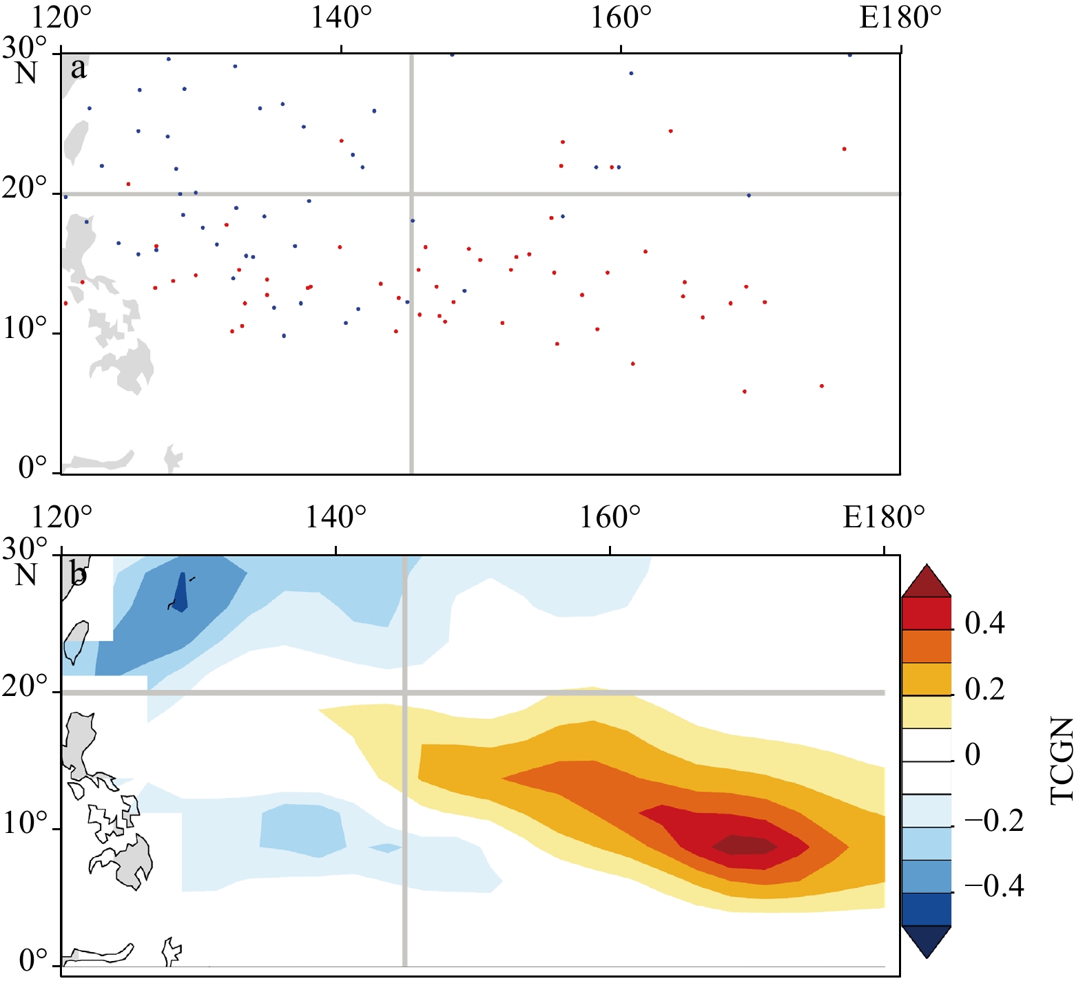
Figure 3. TC genesis during El Niño and La Niña years over the WNP. a. Results from IBTrACS. Red dots and blue dots indicate TC genesis locations in El Niño and La Niña years, respectively. b. Difference in the GPI (derived using ERSSTv5 and NCEP/NCAR reanalysis) between El Niño and La Niña years. Shaded areas represent the 99% confidence level according to the two-tailed Student’s t-test. Zonal gray line at 20°N and meridional line at 145°E divide the WNP into four subregions.
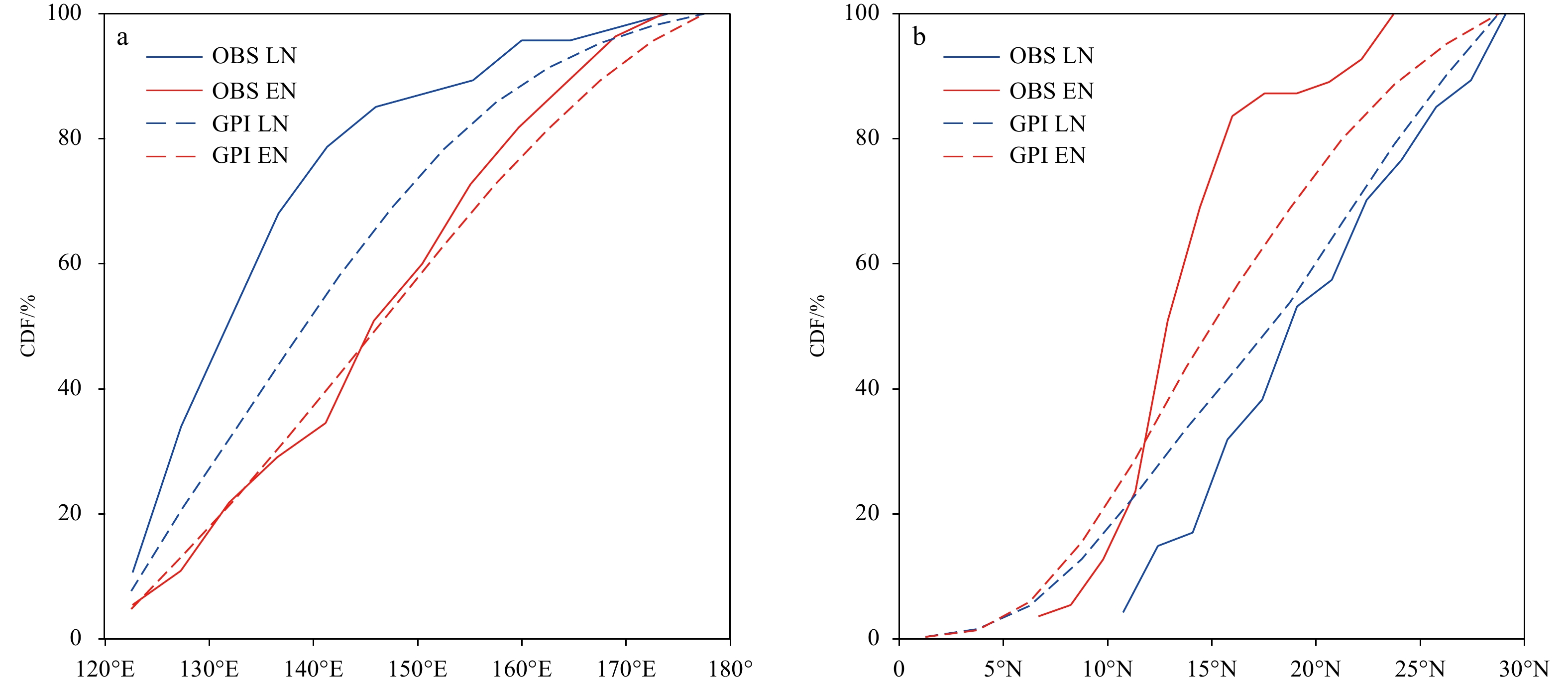
Figure 4. Cumulative distribution function of the longitude (a) and latitude (b) of TC genesis locations over the WNP. Blue and red lines represent the results of La Niña (LN) and El Niño (EN) years, respectively. The observed TC genesis is shown in solid lines and the observed GPIs (derived using ERSSTv5 and NCEP/NCAR reanalysis) are shown in dashed lines.
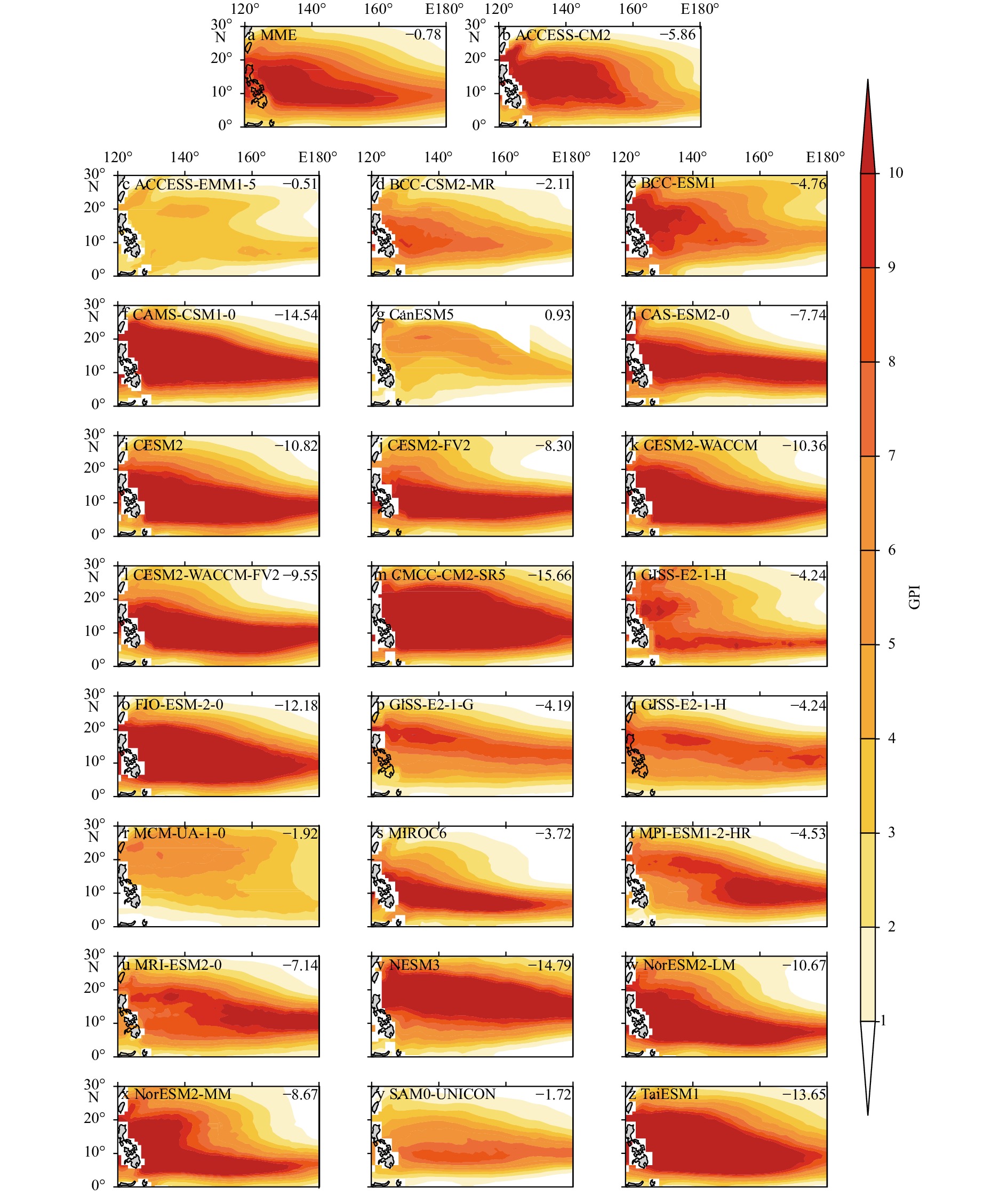
Figure 5. The simulated climatological GPIs over the WNP in CMIP6 models. a. Multi-model ensemble (MME) of 25 CMIP6 models and b–z. simulations in each of 25 CMIP6 models. The skill score of each model is shown on the upper-right corner from a to z.
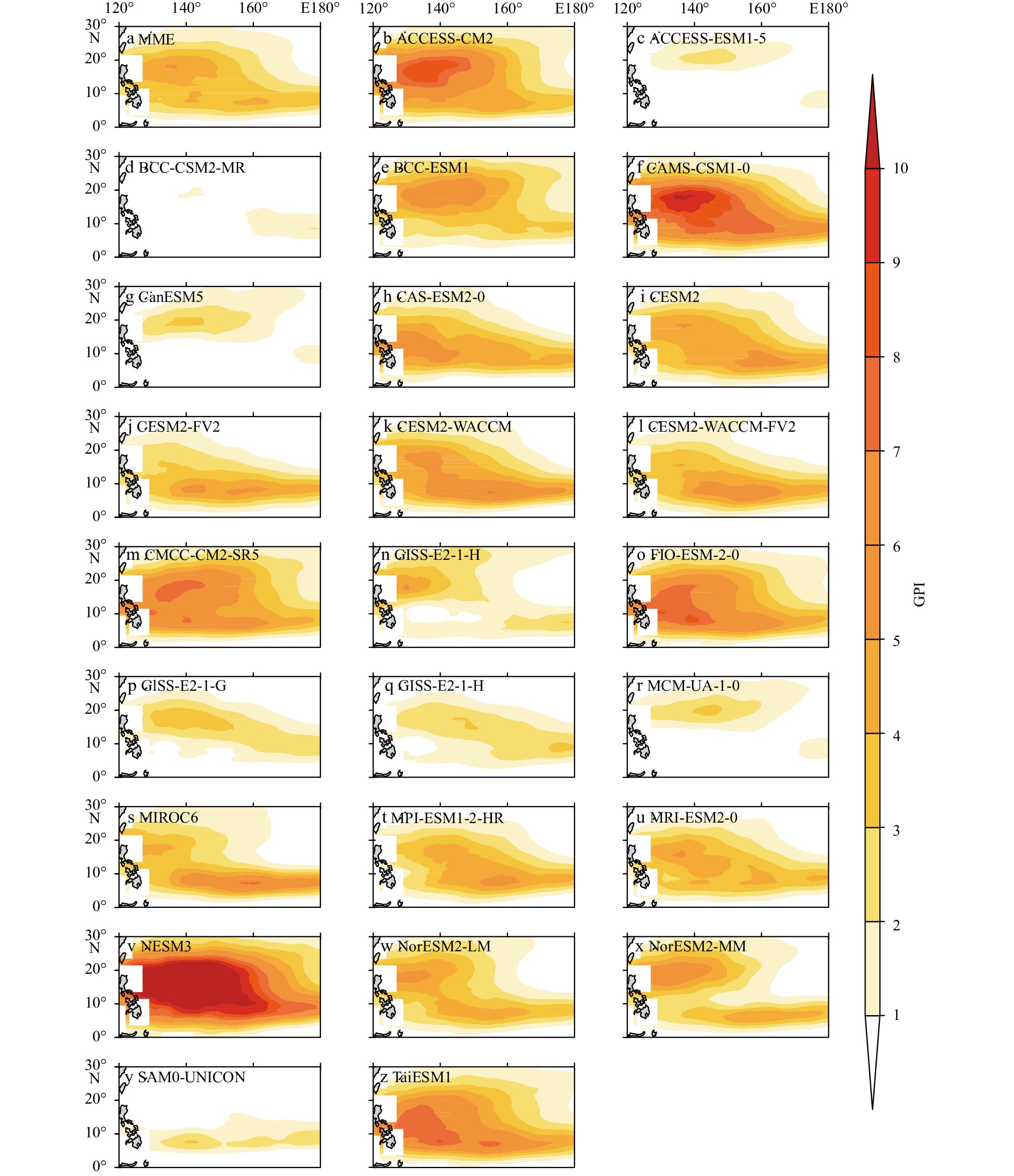
Figure 7. The impacts of the
$ {H}_{600} $ bias on the GPI. a. Ensemble mean impact of 25 CMIP6 models and b–z. impacts for each of 25 CMIP6 models. The impacts shown by shaded areas is statistically significant at the 99% confidence level.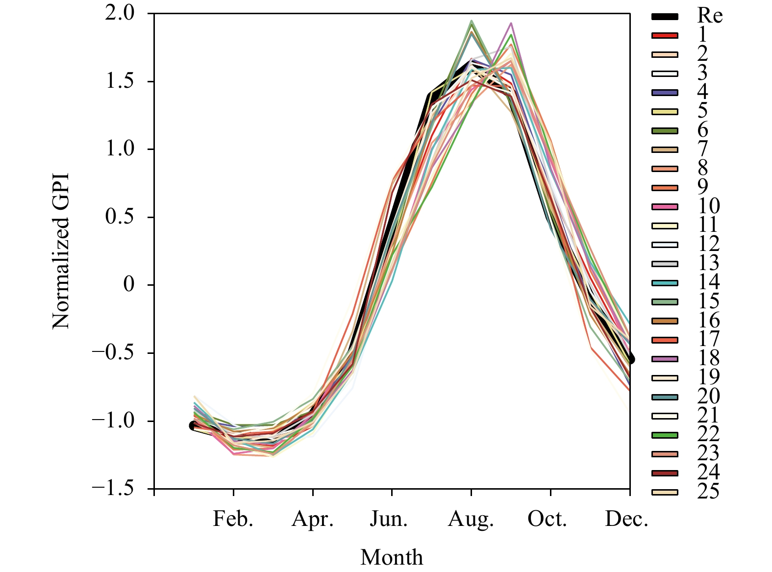
Figure 8. Annual cycle of the observed GPI (thick black line) and the simulated GPIs in 25 CMIP6 models. All GPIs are normalized by subtracting the corresponding climatological mean and dividing by the standard deviation. Numbers in the legend are the serial numbers corresponding to the 25 CMIP6 models in Table 1.

Figure 9. Differences in GPI between El Niño and La Niña years simulated in WMME (a) and PMME (b). Shaded areas represent the 99% confidence level according to the two-tailed Student’s t-test. Contours indicate the difference in the observed GPI (Fig. 3b) between El Niño and La Niña years.

Figure 10. Difference in GPI composites during El Niño and La Niña years caused by varying each variable in Eq. (1). Rows 1–4 show the contribution of low-level vorticity, vertical wind shear, humidity in the mid-troposphere, and potential intensity, respectively. Left column shows the results obtained with ERSSTv5 and NCEP/NCAR reanalysis. Middle column shows the results from the multi-model mean of the well-simulated group. Right column shows the results from the multi-model mean of the poorly simulated group. Shaded areas represent the 99% confidence level according to the two-tailed Student’s t-test. For each panel in the middle and right columns, the CPCCs between the panel and the corresponding observations (the panel on the left column) are shown (purple) in the upper-right corner. For example, the CPCC in b is the correlation coefficient between the pattern in b and the pattern in a.

Figure 11. Differences in SST (a, b), SAT (c, d) and CP (e, f) between El Niño and La Niña years simulated in WMME (a, c, e) and PMME (b, d, f). Shaded areas represent the 99% confidence level according to the two-tailed Student’s t-test. Contours indicate the differences in the SST from ERSSTv5, SAT from NCEP/NCAR reanalysis, and CP from ERA5 between El Niño and La Niña years. The CPCCs between the simulations and the observations are shown (purple) in the upper-right corner.
Table 1. List of the 25 CMIP6 models employed in this study
No. Model Institute ID Resolution (number of grids, lon×lat) Atmosphere Ocean 1 ACCESS-CM2 CSIRO-ARCCSS 192×144 360×300 2 ACCESS-ESM1-5 CSIRO 192×145 360×300 3 BCC-CSM2-MR BCC 320×160 360×232 4 BCC-ESM1 BCC 128×64 360×232 5 CAMS-CSM1-0 CAMS 320×160 360×200 6 CanESM5 CCCma 128×64 361×290 7 CAS-ESM2-0 CAS 256×128 362×196 8 CESM2 NCAR 288×192 320×384 9 CESM2-FV2 NCAR 144×96 320×384 10 CESM2-WACCM NCAR 288×192 320×384 11 CESM2-WACCM-FV2 NCAR 144×96 320×384 12 CMCC-CM2-SR5 CMCC 288×192 362×292 13 FGOALS-g3 CAS 180×80 360×218 14 FIO-ESM-2-0 FIO-QLNM 192×288 320×384 15 GISS-E2-1-G NASA-GISS 144×90 360×180 16 GISS-E2-1-H NASA-GISS 144×90 360×180 17 MCM-UA-1-0 UA 96×80 192×80 18 MIROC6 MIROC 256×128 360×256 19 MPI-ESM1-2-HR MPI-M DWD DKRZ 384×192 802×404 20 MRI-ESM2-0 MRI 320×160 360×364 21 NESM3 NUIST 192×96 384×362 22 NorESM2-LM NCC 144×96 360×384 23 NorESM2-MM NCC 288×192 360×384 24 SAM0-UNICON SNU 288×192 320×384 25 TaiESM1 AS-RCEC 288×192 320×384 Note: CSIRO-ARCCSS: Commonwealth Scientific and Industrial Research Organisation-Australian Research Council Centre of Excellence for Climate System Science; CSIRO: Commonwealth Scientific and Industrial Research Organisation; BCC: Beijing Climate Center; CAMS: Chinese Academy of Meteorological Sciences; CCCma: Canadian Centre for Climate Modelling and Analysis; CAS: Chinese Academy of Sciences; NCAR: National Center for Atmospheric Research; CMCC: Fondazione Centro Euro-Mediterraneo sui Cambiamenti Climatici; FIO-QLNM: First Institute of Oceanography-Ministry of Natural Resources, Qingdao National Laboratory for Marine Science and Technology; NASA-GISS: National Aeronautics and Space Administration-Goddard Institute for Space Studies; UA: University of Arizona-Department of Geosciences; MIROC: Japan Agency for Marine-Earth Science and Technology, Atmosphere and Ocean Research Institute, National Institute for Environmental Studies, RIKEN Center for Computational Science; MPI-M DWD DKRZ: Max Planck Institute for Meteorology, German Meteorological Service, German Climate Computing Center; MRI: Meteorological Research Institute; NUIST: Nanjing University of Information Science and Technology; NCC: Norwegian Climate Centre; SNU: Seoul National University; AS-RCEC: Academia Sinica-Research Center for Environmental Changes.  下载: 导出CSV
Table 2. Centered pattern correlation coefficients (CPCCs) of 25 CMIP6 models with the observed GPIs
Evaluation Model CPCC Well-simulated TaiESM1 0.94 ACCESS-CM2 0.93 FIO-ESM-2-0 0.89 BCC-CSM2-MR 0.88 CESM2-WACCM 0.86 CMCC-CM2-SR5 0.85 NorESM2-LM 0.85 Moderately simulated CESM2 0.83 BCC-ESM1 0.83 CAMS-CSM1-0 0.82 FGOALS-g3 0.81 NorESM2-MM 0.80 SAM0-UNICON 0.79 CESM2-WACCM-FV2 0.79 CESM2-FV2 0.77 ACCESS-ESM1-5 0.77 MIROC6 0.75 CAS-ESM2-0 0.72 Poorly simulated MRI-ESM2-0 0.71 MPI-ESM1-2-HR 0.71 GISS-E2-1-H 0.70 GISS-E2-1-G 0.69 CanESM5 0.65 MCM-UA-1-0 0.51 NESM3 0.48 Note: All CPCCs depict statistical significance based on a two-tailed Student’s t-test (>99%).
下载: 导出CSV
Table 3. R2 difference among CPCCs of WMME, MME, and PMME.
WMME MME PMME WMME (0.93) 0 0.03 0.35 MME (0.91) −0.03 0 0.31 PMME (0.72) −0.35 −0.31 0 Note: Values in bold font were applied to statistically significant differences (two-tailed, p<0.01) based on the Hotelling’s T-squared test and Steiger’s Z-test.
下载: 导出CSV
-
[1] Aiyyer A, Thorncroft C. 2011. Interannual-to-multidecadal variability of vertical shear and tropical cyclone activity. Journal of Climate, 24(12): 2949–2962. doi: 10.1175/2010JCLI3698.1 [2] Bell R, Hodges K, Vidale P L, et al. 2014. Simulation of the global ENSO-tropical cyclone teleconnection by a high-resolution coupled general circulation model. Journal of Climate, 27(17): 6404–6422. doi: 10.1175/JCLI-D-13-00559.1 [3] Bellenger H, Guilyardi E, Leloup J, et al. 2014. ENSO representation in climate models: from CMIP3 to CMIP5. Climate Dynamics, 42(7–8): 1999–2018. doi: 10.1007/s00382-013-1783-z [4] Bister M, Emanuel K A. 1998. Dissipative heating and hurricane intensity. Meteorology and Atmospheric Physics, 65(3–4): 233–240. doi: 10.1007/BF01030791 [5] Bruyère C L, Holland G J, Towler E. 2012. Investigating the use of a genesis potential index for tropical cyclones in the North Atlantic Basin. Journal of Climate, 25(24): 8611–8626. doi: 10.1175/JCLI-D-11-00619.1 [6] Camargo S J. 2013. Global and regional aspects of tropical cyclone activity in the CMIP5 models. Journal of Climate, 26(24): 9880–9902. doi: 10.1175/JCLI-D-12-00549.1 [7] Camargo S J, Barnston A G, Zebiak S E. 2005. A statistical assessment of tropical cyclone activity in atmospheric general circulation models. Tellus A: Dynamic Meteorology and Oceanography, 57(4): 589–604. doi: 10.3402/tellusa.v57i4.14705 [8] Camargo S J, Emanuel K A, Sobel A H. 2007a. Use of a genesis potential index to diagnose ENSO effects on tropical cyclone genesis. Journal of Climate, 20(19): 4819–4834. doi: 10.1175/JCLI4282.1 [9] Camargo S J, Tippett M K, Sobel A H, et al. 2014. Testing the performance of tropical cyclone genesis indices in future climates using the HiRAM model. Journal of Climate, 27(24): 9171–9196. doi: 10.1175/JCLI-D-13-00505.1 [10] Camargo S J, Sobel A H. 2005. Western North Pacific tropical cyclone intensity and ENSO. Journal of Climate, 18(15): 2996–3006. doi: 10.1175/JCLI3457.1 [11] Camargo S, Sobel A H, Barnston A G, et al. 2007b. Tropical cyclone genesis potential index in climate models. Tellus A: Dynamic Meteorology and Oceanography, 59(4): 428–443. doi: 10.1111/j.1600-0870.2007.00238.x [12] Camargo S J, Wheeler M C, Sobel A H. 2009. Diagnosis of the MJO modulation of tropical cyclogenesis using an empirical index. Journal of the Atmospheric Sciences, 66(10): 3061–3074. doi: 10.1175/2009JAS3101.1 [13] Chan J C L. 1985. Tropical cyclone activity in the northwest Pacific in relation to the El Niño/Southern Oscillation phenomenon. Monthly Weather Review, 113(4): 599–606. doi: 10.1175/1520-0493(1985)113<0599:TCAITN>2.0.CO;2 [14] Chan J C L, Liu K S. 2004. Global warming and western North Pacific typhoon activity from an observational perspective. Journal of Climate, 17(23): 4590–4602. doi: 10.1175/3240.1 [15] Chen T C, Weng S P, Yamazaki N, et al. 1998. Interannual variation in the tropical cyclone formation over the western North Pacific. Monthly Weather Review, 126(4): 1080–1090. doi: 10.1175/1520-0493(1998)126<1080:IVITTC>2.0.CO;2 [16] Chia H H, Ropelewski C F. 2002. The interannual variability in the genesis location of tropical cyclones in the northwest Pacific. Journal of Climate, 15(20): 2934–2944. doi: 10.1175/1520-0442(2002)015<2934:TIVITG>2.0.CO;2 [17] Du Yan, Yang Lei, Xie Shangping. 2011. Tropical Indian Ocean influence on northwest Pacific tropical cyclones in summer following strong El Niño. Journal of Climate, 24(1): 315–322. doi: 10.1175/2010JCLI3890.1 [18] Emanuel K A. 1986. An air–sea interaction theory for tropical cyclones. Part I: steady-state maintenance. Journal of the Atmospheric Sciences, 43(6): 585–605. doi: 10.1175/1520-0469(1986)043<0585:AASITF>2.0.CO;2 [19] Emanuel K A. 2013. Downscaling CMIP5 climate models shows increased tropical cyclone activity over the 21st century. Proceedings of the National Academy of Sciences of the United States of America, 110(30): 12219–12224. doi: 10.1073/pnas.1301293110 [20] Emanuel K, Nolan D S. 2004. Tropical cyclone activity and the global climate system. In: Proceedings of the 26th Conference on Hurricanes and Tropical Meteorolgy. Miami, FL: 240–241 [21] Emanuel K, Sundararajan R, Williams J. 2008. Hurricanes and global warming: results from downscaling IPCC AR4 simulations. Bulletin of the American Meteorological Society, 89(3): 347–368. doi: 10.1175/BAMS-89-3-347 [22] Eyring V, Bony S, Meehl G A, et al. 2016. Overview of the coupled model intercomparison project phase 6 (CMIP6) experimental design and organization. Geoscientific Model Development, 9(5): 1937–1958. doi: 10.5194/gmd-9-1937-2016 [23] Frank W M, Ritchie E A. 2001. Effects of vertical wind shear on the intensity and structure of numerically simulated hurricanes. Monthly Weather Review, 129(9): 2249–2269. doi: 10.1175/1520-0493(2001)129<2249:EOVWSO>2.0.CO;2 [24] Fu Dan, Chang Ping, Patricola C M. 2017. Intrabasin variability of East Pacific tropical cyclones during ENSO regulated by central American gap winds. Scientific Reports, 7: 1658. doi: 10.1038/s41598-017-01962-3 [25] Gao Si, Zhu Langfeng, Zhang Wei, et al. 2020. Western North Pacific tropical cyclone activity in 2018: a season of extremes. Scientific Reports, 10(1): 5610. doi: 10.1038/s41598-020-62632-5 [26] Gilford D M, Solomon S, Emanuel K A. 2017. On the seasonal cycles of tropical cyclone potential intensity. Journal of Climate, 30(16): 6085–6096. doi: 10.1175/JCL-D-16-0827.1 [27] Gray W M. 1979. Hurricanes: their formation, structure and likely role in the tropical circulation. In: Shaw D B, ed. Supplement to Meteorology over the Tropical Oceans. Bracknell: James Glaisher House, 155–218 [28] Hagedorn R, Doblas-Reyes F J, Palmer T N. 2005. The rationale behind the success of multi-model ensembles in seasonal forecasting: I. basic concept. Tellus A: Dynamic Meteorology and Oceanography, 57(3): 219–233. doi: 10.3402/tellusa.v57i3.14657 [29] Hersbach H, Bell B, Berrisford P, et al. 2020. The ERA5 global reanalysis. Quarterly Journal of the Royal Meteorological Society, 146(730): 1999–2049. doi: 10.1002/qj.3803 [30] Hoesly R M, Smith S J, Feng Leyang, et al. 2018. Historical (1750–2014) anthropogenic emissions of reactive gases and aerosols from the Community Emissions Data System (CEDS). Geoscientific Model Development, 11(1): 369–408. doi: 10.5194/gmd-11-369-2018 [31] Hotelling H. 1940. The selection of variates for use in prediction with some comments on the general problem of nuisance parameters. Annals of Mathematical Statistics, 11(3): 271–283. doi: 10.1214/aoms/1177731867 [32] Huang Ping, Chou C, Huang Ronghui. 2011. Seasonal modulation of tropical intraseasonal oscillations on tropical cyclone geneses in the western North Pacific. Journal of Climate, 24(24): 6339–6352. doi: 10.1175/2011JCLI4200.1 [33] Huang Boyin, Thorne P W, Banzon V F, et al. 2017. Extended Reconstructed Sea Surface Temperature, Version 5 (ERSSTv5): upgrades, validations, and intercomparisons. Journal of Climate, 30(20): 8179–8205. doi: 10.1175/JCLI-D-16-0836.1 [34] Kalnay E, Kanamitsu M, Kistler R, et al. 1996. The NCEP/NCAR 40-year reanalysis project. Bulletin of the American Meteorological Society, 77(3): 437–472. doi: 10.1175/1520-0477(1996)077<0437:TNYRP>2.0.CO;2 [35] Kim H M, Webster P J, Curry J A. 2011. Modulation of North Pacific tropical cyclone activity by three phases of ENSO. Journal of Climate, 24(6): 1839–1849. doi: 10.1175/2010JCLI3939.1 [36] Klotzbach P J. 2014. The Madden-Julian Oscillation's impacts on worldwide tropical cyclone activity. Journal of Climate, 27(6): 2317–2330. doi: 10.1175/JCLI-D-13-00483.1 [37] Klotzbach P J, Landsea C W. 2015. Extremely intense hurricanes: revisiting Webster et al. (2005) after 10 Years. Journal of Climate, 28(19): 7621–7629. doi: 10.1175/JCLI-D-15-0188.1 [38] Knapp K R, Kruk M C, Levinson D H, et al. 2010. The International Best Track Archive for Climate Stewardship (IBTrACS): unifying tropical cyclone data. Bulletin of the American Meteorological Society, 91(3): 363–376. doi: 10.1175/2009bams2755.1 [39] Knutson T R, McBride J L, Chan J, et al. 2010. Tropical cyclones and climate change. Nature Geoscience, 3(3): 157–163. doi: 10.1038/ngeo779 [40] Knutson T R, Sirutis J J, Garner S T, et al. 2008. Simulated reduction in Atlantic hurricane frequency under twenty-first-century warming conditions. Nature Geoscience, 1(6): 359–364. doi: 10.1038/ngeo202 [41] Knutson T R, Sirutis J J, Vecchi G A, et al. 2013. Dynamical downscaling projections of twenty-first-century Atlantic hurricane activity: CMIP3 and CMIP5 model-based scenarios. Journal of Climate, 26(17): 6591–6617. doi: 10.1175/JCLI-D-12-00539.1 [42] Kowaleski A M, Evans J L. 2015. Thermodynamic observations and flux calculations of the tropical cyclone surface layer within the context of potential intensity. Weather and Forecasting, 30(5): 1303–1320. doi: 10.1175/WAF-D-14-00162.1 [43] Landsea, C W. 2000. El Niño-Southern Oscillation and the seasonal predictability of tropical cyclones. In: El Niño and the Southern Oscillation: Multiscale Variability and Global and Regional Impacts, 149: 181 [44] Li Chunxiang, Wang Chunzai. 2014. Simulated impacts of two types of ENSO events on tropical cyclone activity in the western North Pacific: large-scale atmospheric response. Climate Dynamics, 42(9-10): 2727–2743. doi: 10.1007/s00382-013-1999-y [45] Li R C Y, Zhou Wen. 2013. Modulation of western North Pacific tropical cyclone activity by the ISO: Part I. genesis and intensity. Journal of Climate, 26(9): 2904–2918. doi: 10.1175/JCLI-D-12-00210.1 [46] Lin Jialin. 2007. The double-ITCZ problem in IPCC AR4 coupled GCMs: ocean-atmosphere feedback analysis. Journal of Climate, 20(18): 4497–4525. doi: 10.1175/JCLI4272.1 [47] Lin I I, Chan J C L. 2015. Recent decrease in typhoon destructive potential and global warming implications. Nature Communications, 6: 7182. doi: 10.1038/ncomms8182 [48] Liu K S, Chan J C L. 2008. Interdecadal variability of western North Pacific tropical cyclone tracks. Journal of Climate, 21(17): 4464–4476. doi: 10.1175/2008JCLI2207.1 [49] Makarieva A M, Gorshkov V G, Nefiodov A V, et al. 2017. Fuel for cyclones: the water vapor budget of a hurricane as dependent on its movement. Atmospheric Research, 193: 216–230. doi: 10.1016/j.atmosres.2017.04.006 [50] Maloney E D, Hartmann D L. 2001. The Madden-Julian oscillation, barotropic dynamics, and North Pacific tropical cyclone formation: Part I. observations. Journal of the Atmospheric Sciences, 58(17): 2545–2558. doi: 10.1175/1520-0469(2001)058<2545:TMJOBD>2.0.CO;2 [51] McPhaden M J, Zebiak S E, Glantz M H. 2006. ENSO as an integrating concept in earth science. Science, 314(5806): 1740–1745. doi: 10.1126/science.1132588 [52] Meinshausen M, Vogel E, Nauels A, et al. 2017. Historical greenhouse gas concentrations for climate modelling (CMIP6). Geoscientific Model Development, 10(5): 2057–2116. doi: 10.5194/gmd-10-2057-2017 [53] Menkes C E, Lengaigne M, Marchesiello P, et al. 2012. Comparison of tropical cyclogenesis indices on seasonal to interannual timescales. Climate Dynamics, 38(1–2): 301–321. doi: 10.1007/s00382-011-1126-x [54] Merlis T M, Zhao Ming, Held I M. 2013. The sensitivity of hurricane frequency to ITCZ changes and radiatively forced warming in aquaplanet simulations. Geophysical Research Letters, 40(15): 4109–4114. doi: 10.1002/grl.50680 [55] Mori M, Kimoto M, Ishii M, et al. 2013. Hindcast prediction and near-future projection of tropical cyclone activity over the western North Pacific using CMIP5 near-term experiments with MIROC. Journal of the Meteorological Society of Japan, 91(4): 431–452. doi: 10.2151/jmsj.2013-402 [56] Murphy A H. 1988. Skill scores based on the mean square error and their relationships to the correlation coefficient. Monthly Weather Review, 116(12): 2417–2424. doi: 10.1175/1520-0493(1988)116<2417:SSBOTM>2.0.CO;2 [57] Ooyama K V. 1982. Conceptual evolution of the theory and modeling of the tropical cyclone. Journal of the Meteorological Society of Japan, 60(1): 369–380. doi: 10.2151/jmsj1965.60.1_369 [58] Shen Yixuan, Sun Yuan, Zhong Zhong, et al. 2020. A possible cause of tropical cyclone eastward genesis location bias study using CAM5 model in western North Pacific. Earth and Space Science, 7(1): e2019EA000955. doi: 10.1029/2019EA000955 [59] Shultz J M, Russell J, Espinel Z. 2005. Epidemiology of tropical cyclones: the dynamics of disaster, disease, and development. Epidemiologic Reviews, 27(1): 21–35. doi: 10.1093/epirev/mxi011 [60] Song Yajuan, Wang Lei, Lei Xiaoyan, et al. 2015. Tropical cyclone genesis potential index over the western North Pacific simulated by CMIP5 models. Advances in Atmospheric Sciences, 32(11): 1539–1550. doi: 10.1007/s00376-015-4162-3 [61] Steiger J H. 1980. Tests for comparing elements of a correlation matrix. Psychological Bulletin, 87(2): 245–251. doi: 10.1037/0033-2909.87.2.245 [62] Tan Kexin, Huang Ping, Liu Fei, et al. 2019. Simulated ENSO's impact on tropical cyclone genesis over the western North Pacific in CMIP5 models and its changes under global warming. International Journal of Climatology, 39(8): 3668–3678. doi: 10.1002/joc.6031 [63] Tian Baijun, Dong Xinyu. 2020. The double-ITCZ bias in CMIP3, CMIP5, and CMIP6 models based on annual mean precipitation. Geophysical Research Letters, 47(8): e2020GL087232. doi: 10.1029/2020GL087232 [64] Tian Fangxing, Zhou Tianjun, Zhang Lixia. 2013. Tropical cyclone genesis potential index over the western North Pacific simulated by LASG/IAP AGCM. Acta Meteorologica Sinica, 27(1): 50–62. doi: 10.1007/s13351-013-0106-y [65] Tippett M K, Camargo S J, Sobel A H. 2011. A Poisson regression index for tropical cyclone genesis and the role of large-scale vorticity in genesis. Journal of Climate, 24(9): 2335–2357. doi: 10.1175/2010JCLI3811.1 [66] Walsh K, Lavender S, Scoccimarro E, et al. 2013. Resolution dependence of tropical cyclone formation in CMIP3 and finer resolution models. Climate Dynamics, 40(3–4): 585–599. doi: 10.1007/s00382-012-1298-z [67] Wang Shuguang, Camargo S J, Sobel A H, et al. 2014. Impact of the tropopause temperature on the intensity of tropical cyclones: an idealized study using a mesoscale model. Journal of the Atmospheric Sciences, 71(11): 4333–4348. doi: 10.1175/JAS-D-14-0029.1 [68] Wang Bin, Chan J C L. 2002. How strong ENSO events affect tropical storm activity over the western North Pacific. Journal of Climate, 15(13): 1643–1658. doi: 10.1175/1520-0442(2002)015<1643:HSEEAT>2.0.CO;2 [69] Wang Chunzai, Li Chunxiang, Mu Mu, et al. 2013. Seasonal modulations of different impacts of two types of ENSO events on tropical cyclone activity in the western North Pacific. Climate Dynamics, 40(11–12): 2887–2902. doi: 10.1007/s00382-012-1434-9 [70] Wang Xidong, Liu Hailong. 2016. PDO modulation of ENSO effect on tropical cyclone rapid intensification in the western North Pacific. Climate Dynamics, 46(1–2): 15–28. doi: 10.1007/s00382-015-2563-8 [71] Wang Chunzai, Wang Xin. 2013. Classifying El Niño Modoki I and II by different impacts on rainfall in southern china and typhoon tracks. Journal of Climate, 26(4): 1322–1338. doi: 10.1175/JCLI-D-12-00107.1 [72] Wang Chao, Wang Bin. 2019. Tropical cyclone predictability shaped by western Pacific subtropical high: integration of trans-basin sea surface temperature effects. Climate Dynamics, 53(5–6): 2697–2714. doi: 10.1007/s00382-019-04651-1 [73] Wang Chunzai, Weisberg R H, Virmani J I. 1999. Western Pacific interannual variability associated with the El Niño-Southern Oscillation. Journal of Geophysical Research: Oceans, 104(C3): 5131–5149. doi: 10.1029/1998JC900090 [74] Wang Bin, Yang Yuxing, Ding Qinghua, et al. 2010. Climate control of the global tropical storm days (1965–2008). Geophysical Research Letters, 37(7): L07704. doi: 10.1029/2010GL042487 [75] Watterson I G, Evans J L, Ryan B F. 1995. Seasonal and interannual variability of tropical cyclogenesis: diagnostics from large-scale fields. Journal of Climate, 8(12): 3052–3066. doi: 10.1175/1520-0442(1995)008<3052:SAIVOT>2.0.CO;2 [76] Wengel C, Dommenget D, Latif M, et al. 2018. What controls ENSO-amplitude diversity in climate models?. Geophysical Research Letters, 45(4): 1989–1996. doi: 10.1002/2017GL076849 [77] Wing A A, Emanuel K, Solomon S. 2015. On the factors affecting trends and variability in tropical cyclone potential intensity. Geophysical Research Letters, 42(20): 8669–8677. doi: 10.1002/2015GL066145 [78] Wu Qiong, Zhao Jiuwei, Zhan Ruifen, et al. 2021. Revisiting the interannual impact of the Pacific Meridional Mode on tropical cyclone genesis frequency in the western North Pacific. Climate Dynamics, 56(3–4): 1003–1015. doi: 10.1007/s00382-020-05515-9 [79] Yamasaki M. 2007. A view on tropical cyclones as CISK. Journal of the Meteorological Society of Japan, 85B: 145–164. doi: 10.2151/jmsj.85B.145 [80] Yan Qing, Korty R, Zhang Zhongshi, et al. 2019. Evolution of tropical cyclone genesis regions during the Cenozoic era. Nature Communications, 10(1): 3076. doi: 10.1038/s41467-019-11110-2 [81] Yang Lei, Chen Sheng, Wang Chunzai, et al. 2018a. Potential impact of the Pacific Decadal Oscillation and sea surface temperature in the tropical Indian Ocean-Western Pacific on the variability of typhoon landfall on the China coast. Climate Dynamics, 51(7–8): 2695–2705. doi: 10.1007/s00382-017-4037-7 [82] Yang Mengmiao, Zhang G J, Sun Dezheng. 2018b. Precipitation and moisture in four leading CMIP5 models: biases across large-scale circulation regimes and their attribution to dynamic and thermodynamic factors. Journal of Climate, 31(13): 5089–5106. doi: 10.1175/JCLI-D-17-0718.1 [83] Yokoi S, Takayabu Y N, Chan J C L. 2009. Tropical cyclone genesis frequency over the western North Pacific simulated in medium-resolution coupled general circulation models. Climate Dynamics, 33(5): 665–683. doi: 10.1007/s00382-009-0593-9 [84] Yonekura E, Hall T M. 2011. A statistical model of tropical cyclone tracks in the western North Pacific with ENSO-dependent cyclogenesis. Journal of Applied Meteorology and Climatology, 50(8): 1725–1739. doi: 10.1175/2011JAMC2617.1 [85] Yonekura E, Hall T M. 2014. ENSO effect on East Asian tropical cyclone landfall via changes in tracks and genesis in a statistical model. Journal of Applied Meteorology and Climatology, 53(2): 406–420. doi: 10.1175/JAMC-D-12-0240.1 [86] Zhang G J, Song Xiaoliang, Wang Yong. 2019. The double ITCZ syndrome in GCMs: a coupled feedback problem among convection, clouds, atmospheric and ocean circulations. Atmospheric Research, 229: 255–268. doi: 10.1016/j.atmosres.2019.06.023 期刊类型引用(1)
1. Han-Kyoung Kim, Jong-Yeon Park, Doo-Sun R. Park, et al. Western North Pacific tropical cyclone activity modulated by phytoplankton feedback under global warming. Nature Climate Change, 2024.  必应学术
必应学术其他类型引用(0)
-


 DownLoad:


 必应学术
必应学术 点击查看大图
计量
- 文章访问数: 1193
- HTML全文浏览量: 481
- PDF下载量: 62
- 被引次数: 1

