


Figure
1.
Global high-resolution ocean reanalysis product CORA v2.0 data information.
| Citation: | Tao Shiyuan, Yu Yi, Xiao Wenbin, Zhang Weimin, Zhao Yanlai. Analysis of the distribution of sound velocity profiles and sound propagation laws based on a global high-resolution ocean reanalysis product[J]. Acta Oceanologica Sinica.

|
As the only known signal carrier capable of long-distance transmission in the ocean (Yang, 1998), sound waves are one of the best choices for us to continuously understand and utilize the ocean. High-resolution sound velocity profile data help obtain detailed acoustic information about the ocean, thus enhancing the capability and level of ocean environmental data assurance. By assimilating historical observation data with dynamic model integration through ocean reanalysis products (Wu et al., 2022), we can reproduce past changes in the ocean state field, providing convenience for accurate oceanic environmental and acoustic research and greatly promoting the development of marine science and technology.
Ocean reanalysis research is highly valued in the international marine field, with countries such as the United States, Europe, France, the United Kingdom, Japan, and Australia having their own ocean reanalysis programs. Among them, the United States' Estimating the Circulation and Climate of the Ocean (ECCO) (Feng et al., 2021), Simple Ocean Data Assimilation (SODA) (Duan et al., 2016), Hybrid Coordinate Ocean Model (HYCOM) (Pottapinjara and Joseph, 2022), Europe's Ocean Reanalysis System (ORAS4) (Balmaseda et al., 2013), and other ocean reanalysis products have significant international influence and have been widely applied in areas such as ocean environmental security, marine science, and climate change research.
In 2009, the China National Marine Data and Information Service (NMDIS) released the CORA experimental version of ocean reanalysis products. In 2018, the CORA v1.0 global and Northwest Pacific regional ocean reanalysis product was published, achieving operational updates (Chao et al., 2021). From 2016 to 2020, the China National Marine Data and Information Service, in collaboration with multiple institutions, pioneered the development of the CORA v2.0 global 1/12° high-resolution ice-ocean coupled reanalysis product, which includes tides.
In 2013, Han Guijun et al. (Han et al., 2013) evaluated the CORA trial product and found that the annual mean heat content of the CORA dataset was very close to that of the 2009 World Ocean Atlas (WOA09) data compared with modeled simulations. In terms of the quality of global climatology, it was comparable to the Simple Ocean Data Assimilation (SODA) product, and it reconstructed major ENSO events. In 2015, Balmaseda et al. initiated the Ocean Reanalysis Intercomparison Project (ORA-IP) (Balmaseda et al., 2015) to compare multiple global ocean reanalysis products and describe the characteristics of different reanalysis products, as well as point out the deficiencies of current reanalysis products and future development directions. In 2016, Zhang Min, Zhou Lei et al. (Zhang et al., 2016) compared the CORA trial product with ECCO2 and SODA, evaluated the seasonal variability of CORA, and found that CORA performed better than ECCO2 and SODA in capturing seasonal sea surface temperature (SST) and sea surface height (SSH). In 2019, Fan Maoting (Fan et al., 2020) conducted relevant research on the application of the CORA v1.0 product in the South China Sea, demonstrating the availability of the CORA v1.0 product in the South China Sea, but also pointing out that the accuracy of the dataset needs further improvement. In 2021, Li Zhijie, Wang Zhaoyi et al. (Li et al., 2021) compared and evaluated the climate state product of the China Global Ocean Forecasting System (CGOFS) with internationally recognized World Ocean Atlas (WOA), Simple Ocean Data Assimilation (SODA), and other ocean data products, and showed that the climate state results of CGOFS were basically consistent with similar international products. In the same year, Guofang Chao et al (Chao et al., 2021) developed and verified a new reanalysis product based on the 51-year (1958-2008) CORA v1.0 product and found that the new reanalysis product had good representativeness for the actual ocean conditions in the Northwest Pacific.
Since the release of the trial version, the CORA series of ocean reanalysis products have attracted wide attention. However, there is currently a lack of evaluation and analysis on CORA v2.0, a new generation of high-resolution ocean reanalysis products independently developed in China. In order to fully test the performance of CORA v2.0 and explore its application prospects, this study selects six typical global ocean locations and compares them with Argo float observation data, as well as two commonly used reanalysis data sources: generalized digital environment model (GDEM) and world ocean atlas (WOA). Furthermore, the global spatiotemporal distribution characteristics of ocean sound speed are studied using CORA v2.0 data.
(1) Argo
The Argo program, initiated in the late 20th century, was jointly established by multiple countries including China. It has now become a real-time data observation platform covering global oceans, providing over a million temperature and salinity profiles to the world (Yu and Wu, 2021). The Argo program focuses on measuring seawater profiles from 0 to 2000 meters, which is of great significance in improving our understanding of the three-dimensional structure of the upper and middle layers of the ocean (Johnson et al., 2022). The observation system consists of approximately
(2) GDEM
The general digital environmental model was developed by the United States Navy and is a global monthly average oceanographic dataset used for environmental protection by the US Navy (Carnes et al., 2010). Its spatial resolution is 0.25 x 0.25 degrees; it is divided into 689 grid points in the latitude direction, covering a range from −82.0° to 90.0°; in the longitude direction, it is divided into
(3) WOA
The world ocean atlas (WOA) is a set of climate-averaged gridded fields of oceanic variables, established based on field measurement data from various sources (Li et al., 2019). WOA data include multiple versions, with seasonal and monthly averages for each year. This study utilized 2013 monthly average data from WOA13. The latitude range for WOA13 data is from 89.5°S to -89.5°N, the longitude range is from -179.5°W to 179.5°E, and it has 33 vertical levels with a maximum depth of
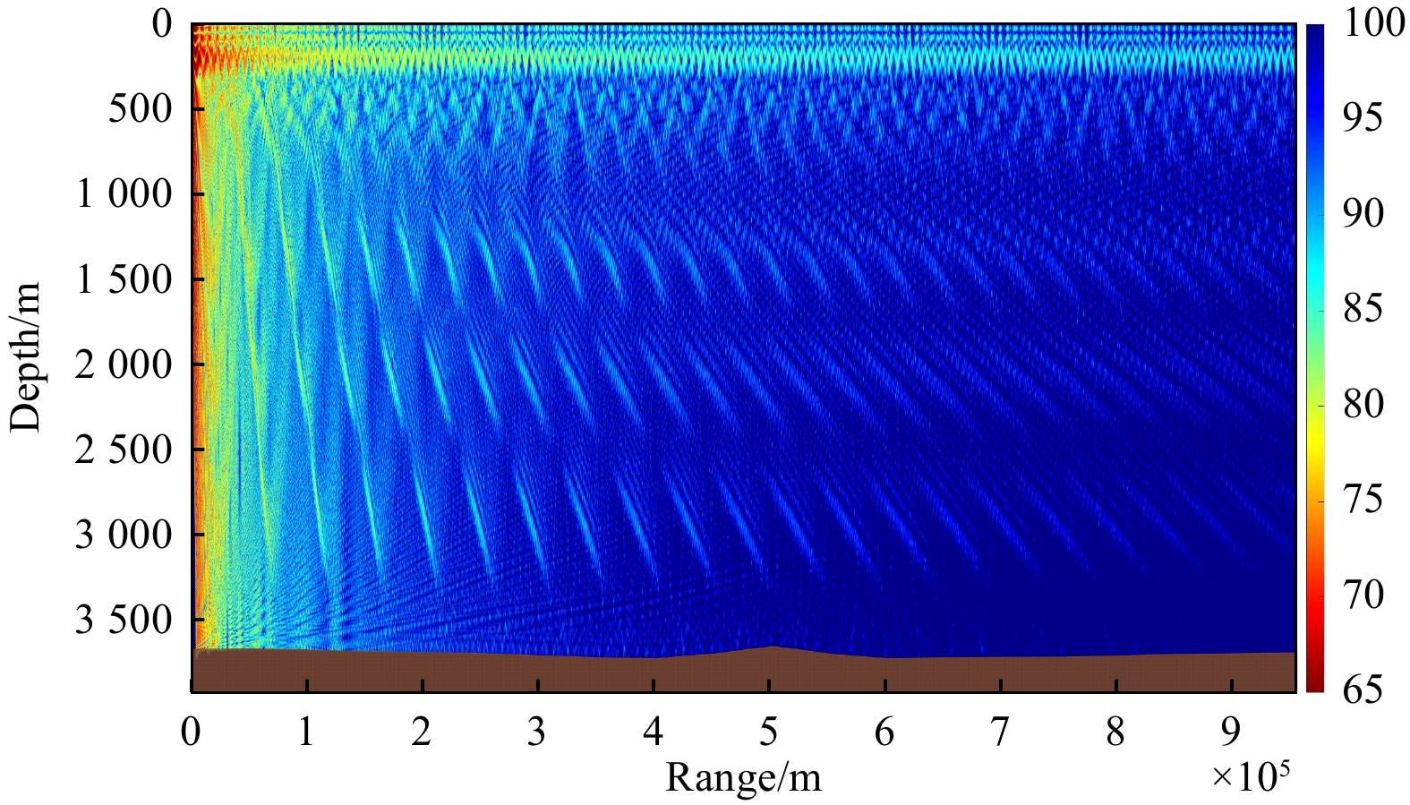
CORA v2.0 includes ocean reanalysis elements such as sea surface height, temperature, salinity, ocean currents, effective wave height and mean period, sea ice concentration, thickness, and drift speed. Assimilated data consist of in situ temperature and salinity observations, as well as remote sensing observations. The numerical model involves combining the ocean circulation model (MITgcm) with the sea ice module (Community Ice Code, CICE). The data have a horizontal resolution of 0.1° × 0.1° and a vertical resolution of 50 layers. CORA v2.0 offers products with various temporal resolutions (monthly average data products, daily average data products, and high temporal resolution data products at 3-hour intervals). The reanalysis period covers no less than 30 years (from 1980 to 2020) and is updated annually (Fu et al., 2023), providing important data information for marine environmental scientific research.
In the process of acoustic analysis, the temperature and salinity data elements of seawater are usually of particular interest. In CORA v2.0 data, the variable names for these two categories are THETA and SALT, respectively. The dimensions of these data are
In the western Pacific, South Pacific, South China Sea, the Arabian Sea, the Indian Ocean, and the Arctic Ocean, one point is selected from each region for comparative data analysis and spatiotemporal distribution pattern analysis of sound speed. Among them, Point A is located in the control area of the subtropical high-pressure system in the western Pacific, with distinct climate characteristics; Point B is located in the South Pacific, with minimal influence from land and a unique marine environment; Point C is located in the South China Sea, which has very rich marine resources; Point D is located in the northern Indian Ocean, an important sea route for East Asian countries; Point E is located in the Arabian Sea, which is of significant importance for international security issues and humanitarian actions; and Point F is located in the Arctic Ocean, with a unique marine environment and important scientific research value for polar marine environmental exploration. The depths and positions of each point are listed in Table 1.
| Point | Depth/m | Position |
| A | 11.55°N, 130.95°E | |
| B | 39.55°S, 147.35°W | |
| C | 18.15°N, 117.95°E | |
| D | 5.25°N, 86.05°E | |
| E | 150.8 | 11.65°N, 43.55°E |
| F | 75.45°N, 144.05°W |
 DownLoad:
CSV
DownLoad:
CSV
The sound speed values of the three reference datasets, Argo, GDEM, and WOA, were interpolated to the standard layers of CORA v2.0. Equation (1) was used to calculate the offsets, average offset, and root mean square error between the different datasets. Based on these calculations, a comparative analysis was conducted.
| $$ {E_i} = {X_{CORAv2.0}}(i) - {X_{{Re} f}}(i) $$ | (1) |
| $$ ME = \frac{{\displaystyle\sum {{E_i}} }}{n} $$ | (2) |
| $$ RMSE = \sqrt {\frac{{\displaystyle\sum {E_i^2} }}{n}} , $$ | (3) |
where Ei represents the offset, ME represents the average offset, RMSE represents the root mean square error, and i indicates the vertical layer.
When conducting a comparative analysis between Argo and CORA v2.0 data, due to the uncertainty in the distribution of Argo float positions, we identified Argo data close to the selected points for comparison through calculation. In this section, we select data from Points A, C, and D in Figure 2 at three different time points in 2014 for comparative testing.

Figure 3 shows a comparison of sound speed profiles between CORA v2.0 data and Argo data at Point A in the western Pacific at 21:00 on January 28, 21:00 on February 7, and 03:00 on April 30. The figure shows that at these three time points, the sound speed profile at this point represents the deep-sea sound channel sound speed distribution type (Liu et al., 2020). The depth of the sea surface mixed layer was approximately between 0 and 100 meters, and the depth range of the sound speed interface was approximately between 100 and 300 meters. The sound speed profile using CORA v2.0 data was smoother above the sound speed interface compared to that of Argo data, while there were still significant fluctuations below the sound speed interface. At these three moments, the average offset between CORA v2.0 data and Argo data was within ±2 m/s, and the root mean square error was within 3 m/s.

| Moment | 2014-01-28 21:00 | 2014-02-07 21:00 | 2014-04-30 03:00 |
| ME | − |
− |
|
| RMSE |
DownLoad:
CSV
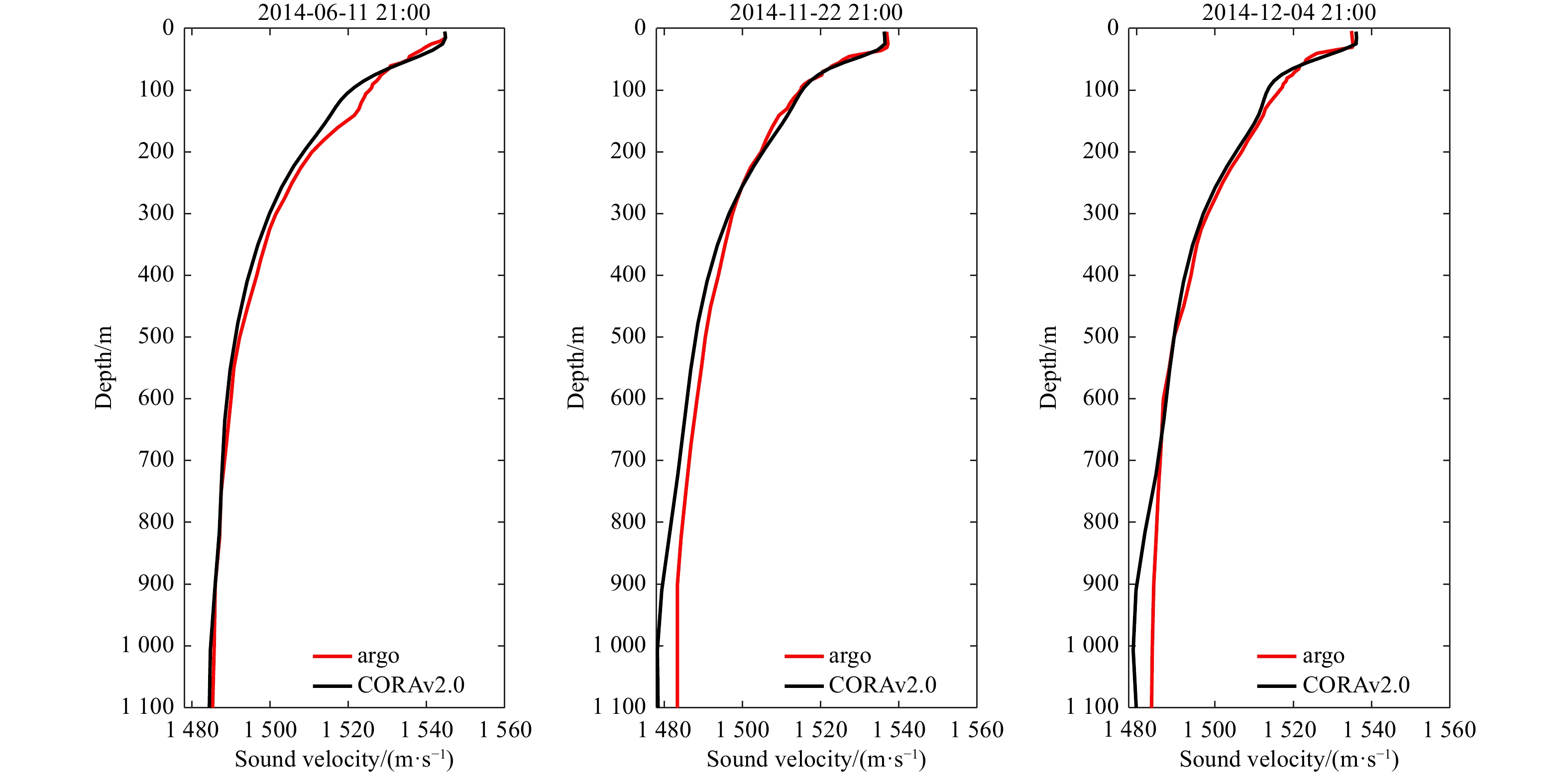
Figure 4 presents a comparison of sound speed profiles between Argo data and CORA v2.0 data at Point C in the South China Sea at three different time points: June 11th at 21:00, November 22nd at 21:00, and December 4th at 21:00. The figure shows that there were significant fluctuations in the difference between CORA v2.0 data and Argo data near the sea surface. This was mainly due to the influence of multiple factors on the sea surface, resulting in strong data instability and larger fluctuations in Argo data near the sea surface. From a quantitative perspective, the average offset and root mean square error of sound speed were highest at 21:00 on June 11th, while they were lowest at 21:00 on November 22nd. The average offsets at all three time points were within ±2 m/s, and the root mean square errors were within 3 m/s.
| Moment | 2014-05-11 21:00 | 2014-11-22 21:00 | 2014-12-04 21:00 |
| ME | − |
− |
− |
| RMSE |
DownLoad:
CSV
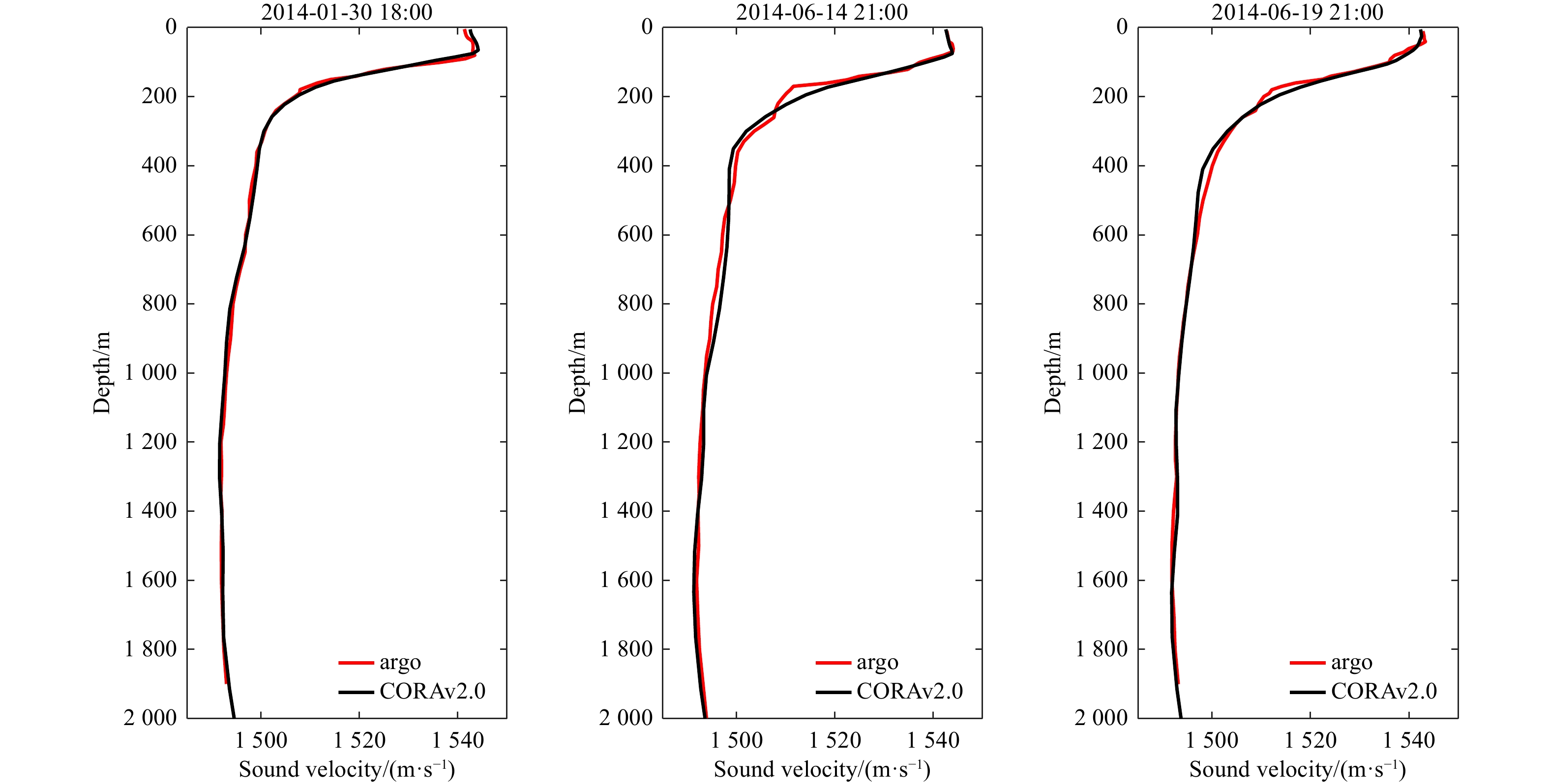
Figure 5 shows a comparison of Argo data and CORA v2.0 data sound speed profiles at three time points: January 30th at 6:00 pm, June 14th at 9:00 pm, and June 19th at 6:00 pm in the Indian Ocean at Point D. The figure shows that the Argo data fluctuated significantly near the shallow sea and thermocline, with large differences compared to the CORA v2.0 data. The sound speed profile structure was generally similar to Points A and C mentioned above. In terms of average offset and mean square error, the average offset and mean square error were smallest at 6:00 pm on January 30th, with an average offset of less than 0.1 m/s. The deviation was largest at 9:00 pm on June 14th, but the average offset and mean square error were only
| Moment | 2014-01-30 18:00 | 2014-06-14 21:00 | 2014-06-19 18:00 |
| ME | − |
||
| RMSE |
DownLoad:
CSV
For the three datasets with monthly average data products, CORA v2.0, WOA, and GDEM, the monthly average sound speed data at the six mentioned locations were selected for comparative analysis. According to Equation (3), the sound speed differences and mean square errors of these three datasets were calculated, and the monthly variations in 2013 were investigated.
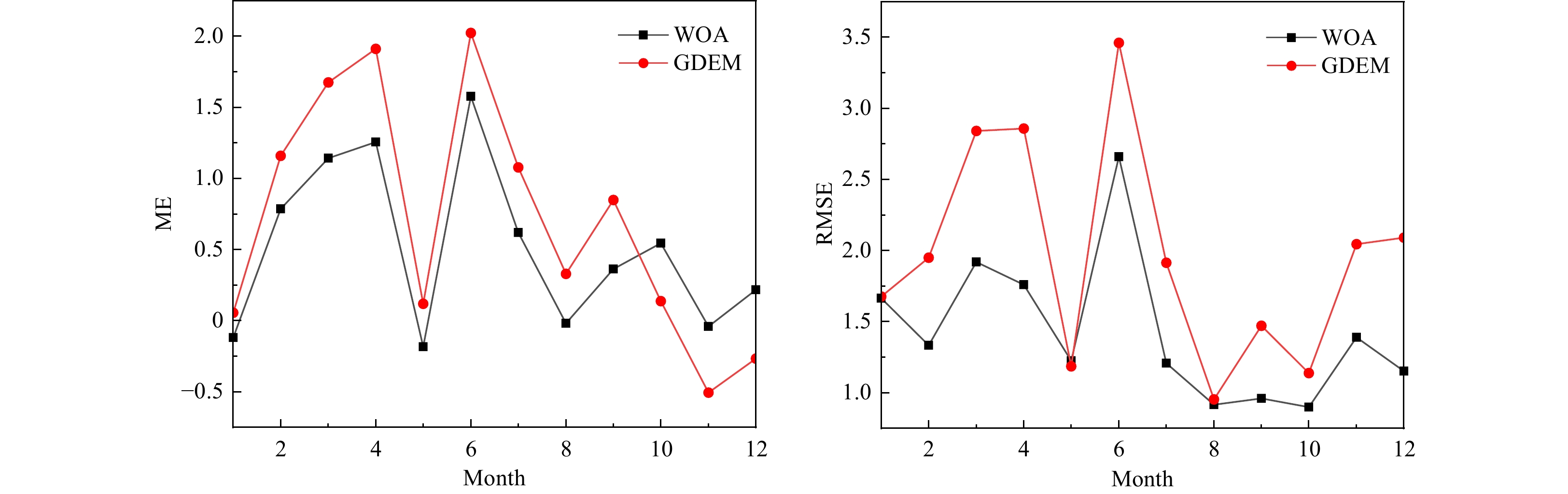
From a comparison of monthly average sound speed errors at Point A in the western Pacific in Figure 6, it can be seen that in the shallow sea, CORA v2.0 data were greater than the reference dataset. At depths of
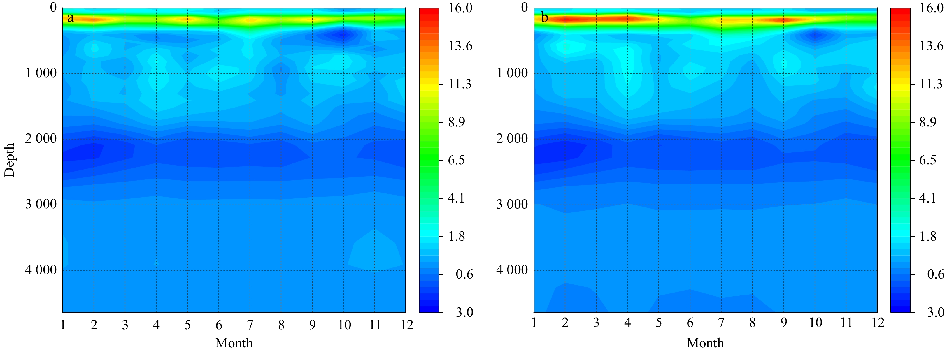
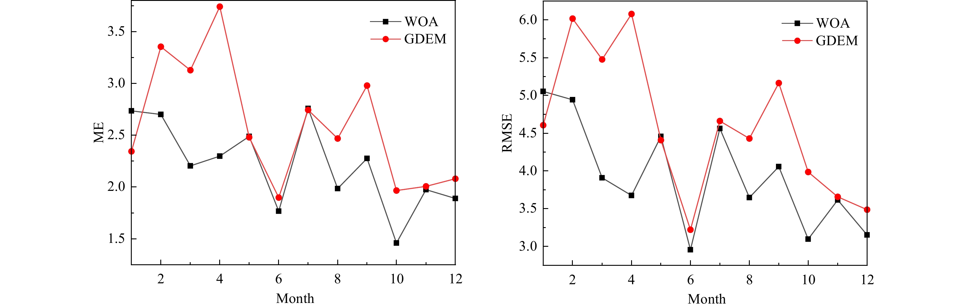
Figure 8 shows that there was significant fluctuation in the sound speed differences between CORA v2.0 and the two reference datasets, WOA and GDEM, in the shallow sea area. At depths of 2000-
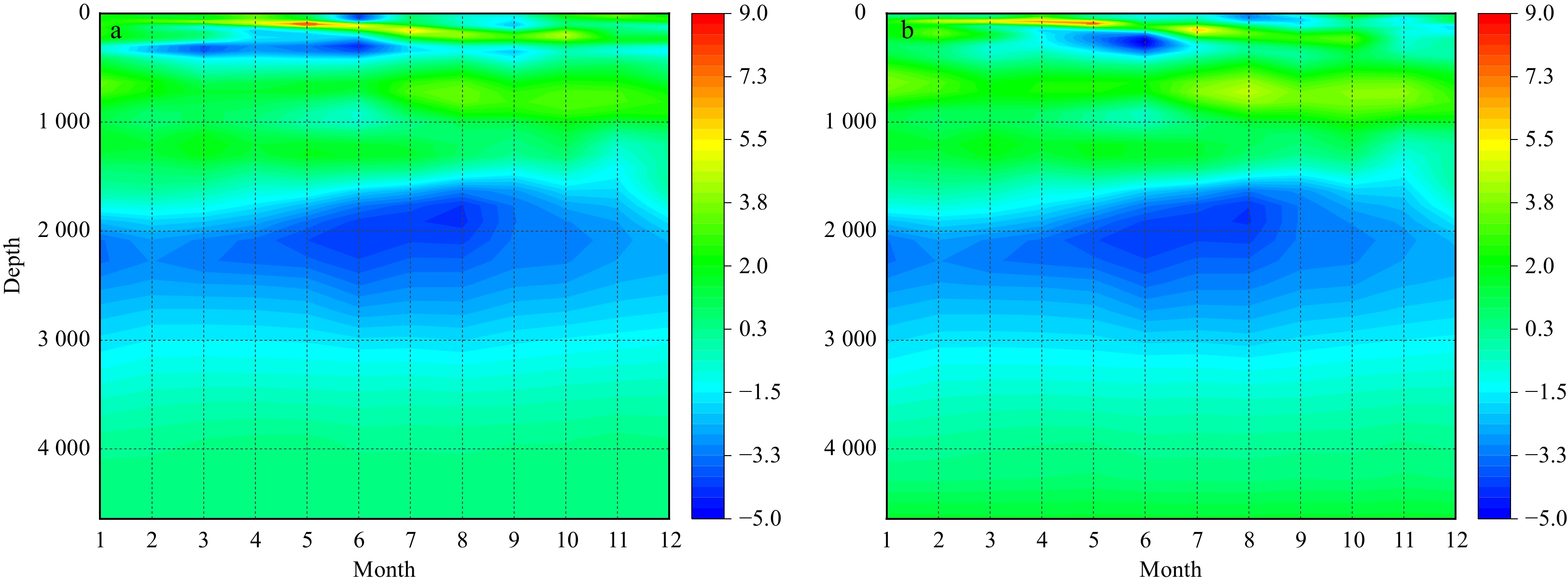
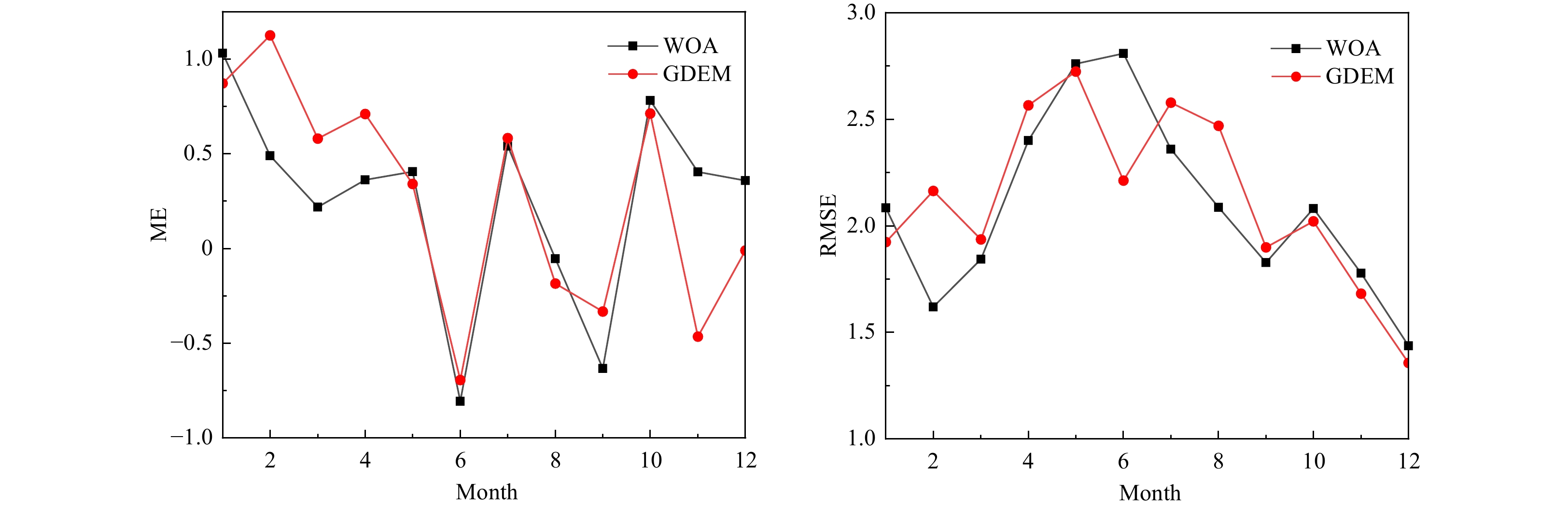
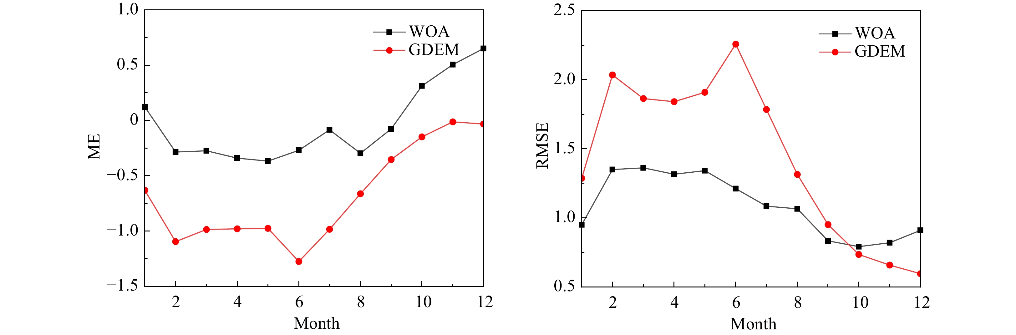
Figure 10 shows that in waters deeper than 500 m at Point C in the South China Sea, CORA v2.0 exhibited significant fluctuations in difference compared to the reference dataset over time. The fluctuations decreased in waters shallower than 500 meters, and the difference gradually approached 0 m/s with increasing depth. Figure 11 shows that the annual variation trend of the average deviation and mean square error in the CORA v2.0 dataset was generally consistent with the reference dataset. Additionally, CORA v2.0 data had a larger average deviation compared to the GDEM data. This indicates that at this specific location, CORA v2.0 dataset showed consistent differences with the two reference datasets, particularly showing good agreement with WOA.
According to Figure 12, the difference between the CORA v2.0 data and the reference dataset also had significant fluctuations in shallow waters. The maximum and minimum values occurred in June and November, respectively. From a quantitative analysis perspective, the sound speed values in the CORA v2.0 dataset were mostly higher than those in the two reference datasets throughout the year. In January and May, the sound speed values in the CORA v2.0 dataset were slightly lower than those in the two reference datasets, with a minimum value occurring in May. The trend of the average deviation of the sound speed profiles between the CORA v2.0 dataset and the two reference datasets was generally consistent for most months, except for October, November, and December. The average deviation of the CORA v2.0 dataset relative to the GDEM dataset was larger than that relative to the WOA dataset, except for these months. The mean square error between the CORA v2.0 dataset and the two reference datasets also indicated that the CORA v2.0 dataset had a larger error compared to that of the GDEM dataset, while the deviation was smaller compared to that of the WOA dataset.

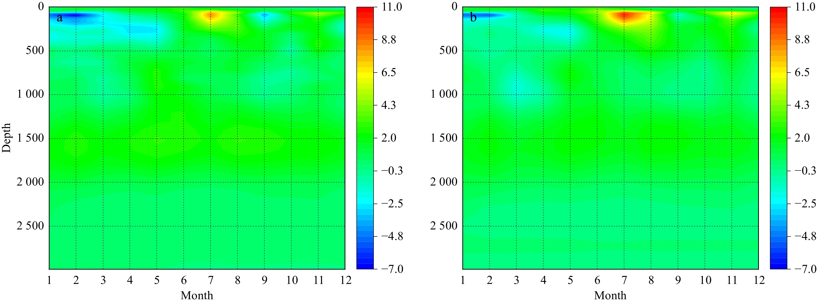
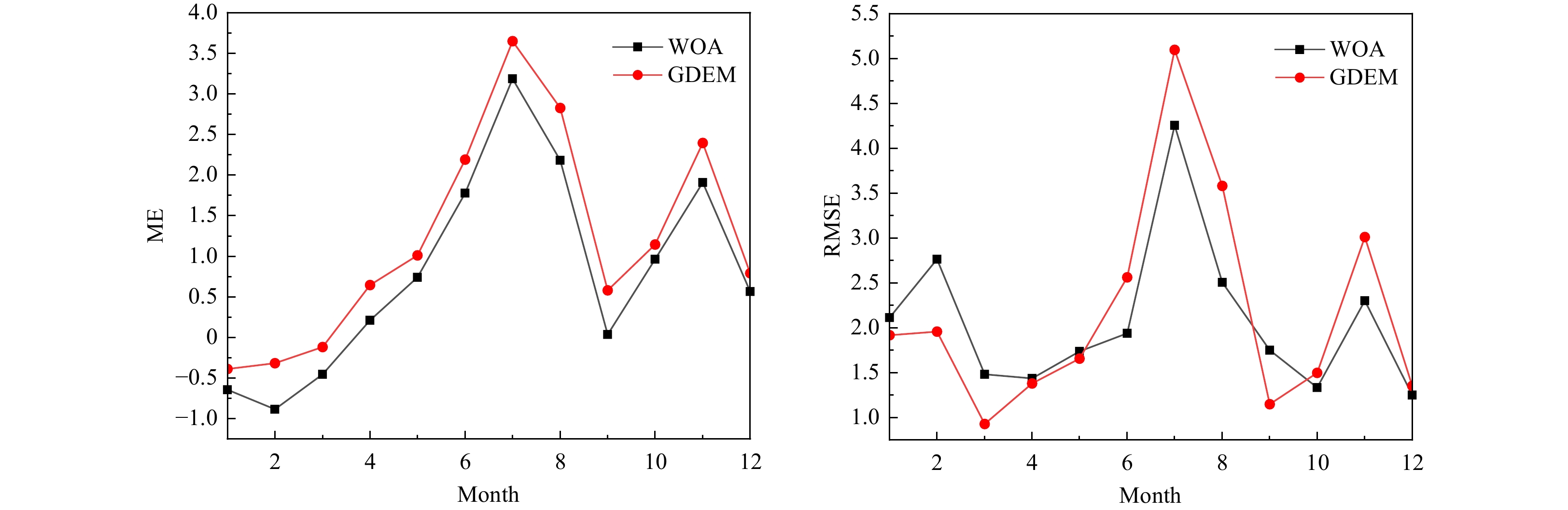
Point E is located in the Gulf of Aden and has shallower depths compared to other points, which allows it to demonstrate the differences among the three datasets in shallow waters. According to Figure 14, the difference in sound velocity values between the datasets in the surface seawater fluctuated less, while at a depth of 80 meters, there was a significant fluctuation in the sound velocity difference. Figure 15 shows that compared to Points A, B, C, and D mentioned above, Point E had a larger average deviation and mean square error. Especially in some months, the average deviation between CORA v2.0 and the GDEM dataset could even reach close to 10 m/s. Additionally, except for September and October, the CORA v2.0 dataset overall had larger values compared to the other two reference datasets. Apart from a peak in June, the overall trend of the average deviation and mean square error between these two sets of data in other months was generally consistent.


According to Figure 16, similar to the aforementioned points, the difference in sound velocity between the CORA v2.0 dataset and the reference datasets was more pronounced in the shallow area. The sound velocity difference between the CORA v2.0 dataset and the WOA and GDEM reference datasets reached its minimum values continuously from February to July. The difference between CORA v2.0 and WOA was relatively small (Figure 16a), while the difference between CORA v2.0 and GDEM was relatively large (Figure 16b). This may be related to Point F being located within the Arctic Circle, where it experiences phenomena such as polar day and polar night due to variations in solar radiation. Below a depth of

The above detailed comparative analysis of the CORA v2.0 dataset with three types of data, Argo, GDEM, and WOA, was conducted from the perspective of sound velocity. Comparing the CORA v2.0 dataset with the Argo data, it can be observed that the sound velocity profiles of the two datasets had some differences, but the overall difference was small, with more noticeable fluctuations in shallow waters. The average deviation remained within ±2 m/s, and the mean square error remained below 3 m/s. It can be concluded that the CORA v2.0 dataset exhibits good consistency with the Argo dataset.
Comparing the CORA v2.0 dataset with foreign ocean reanalysis data products, GDEM and WOA, it can be seen that the average deviation and mean square error between CORA v2.0 and the two reference datasets exhibit similar trends over time, with better consistency between CORA v2.0 and WOA.
The analysis of the CORA v2.0 data above to some extent demonstrates its practical value and reliability. Next, we use the CORA v2.0 data to analyze the spatiotemporal patterns of global sound speed distribution.
Based on the above research work, the CORA v2.0 data at 12:00 on January 15, 2014 were selected for the spatial distribution characteristics analysis of global seawater sound speed.
The sound speed in the upper layer of the global ocean has a zonal distribution characteristic (as shown in Figure 18): the sound speed gradually decreases from low latitudes to high latitudes, with the highest sound speed near the equator; the sound speed is lowest in the polar regions; and the sound speed distribution in the Indian Ocean, western Pacific Ocean, and Arctic Ocean is relatively uniform, with no significant fluctuations in sound speed values. However, in some areas of the eastern Pacific Ocean and the Atlantic Ocean, there are significantly irregular fluctuations in sound speed, which may be closely related to small-scale phenomena in the upper ocean and surface currents.

As depth increases, the sound speed shows a decreasing trend (as shown in Figures 18, 19, 20, and 21), with the most obvious changes in the mid–low-latitude regions, and a slight increase in sound speed values in high-latitude regions as depth increases. When depth reaches a certain level, the distribution of temperature-with-latitude changes basically disappears, and the global seawater sound speed distribution becomes relatively uniform, with higher sound speed values in the northeastern part of the Atlantic Ocean and some parts of the Indian Ocean, while sound speed values in other areas remain mostly below
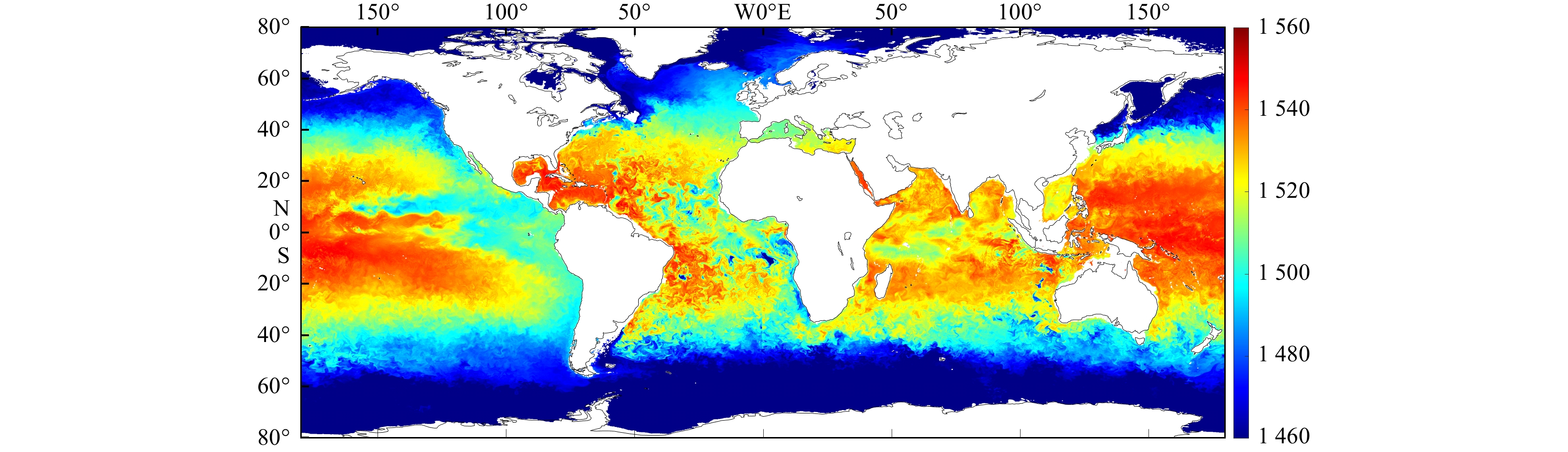


It is worth mentioning that due to factors such as geographical location, the sound speed values in the Mediterranean Sea and the Red Sea do not show significant changes with depth. The Red Sea is relatively enclosed, surrounded by desert terrain, with limited inflow of freshwater from the outside, and due to the influence of seafloor topography, the exchange of deep-sea water with the outside world is more difficult. Located near the Tropic of Cancer, the Red Sea is influenced by subtropical high pressure, with low annual rainfall, high evaporation at the sea surface, and multiple combined factors leading to high salinity, which in turn affects its sound speed distribution (Zhao et al., 2019).
To better examine the practicality of CORA v2.0 data and understand the annual variation patterns of sound speed profiles in specific ocean areas, an analysis of the temporal scale of sea water sound speed variations was conducted using the six designated points. The CORA v2.0 data with a temporal resolution of 3 hours were used to plot the sound speed–depth structure at these points for of 2014, totaling
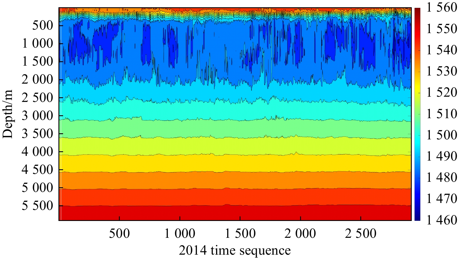


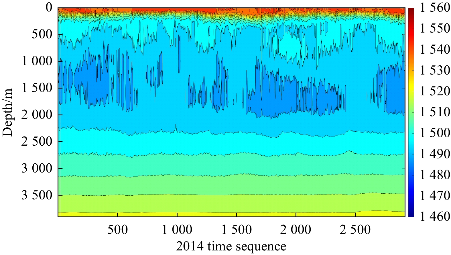
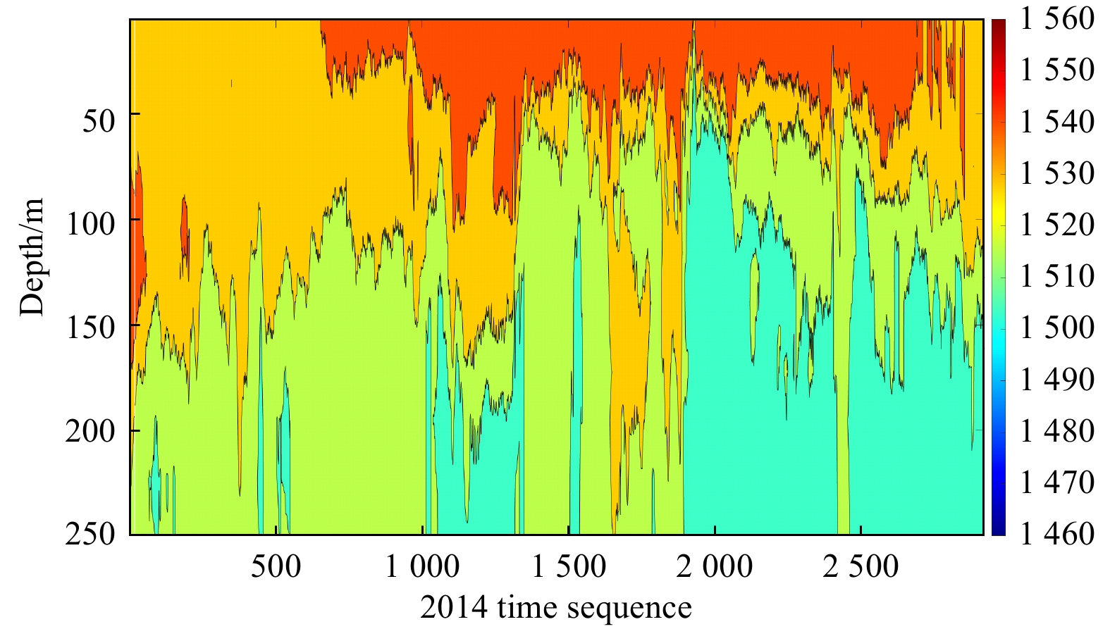

The figures show that there is a significant annual variation in sound speed in the upper and middle layers of the ocean, with variations differing depending on latitude and geographical location. The sound speed in the lower layer of the ocean generally maintains a stable layered structure. Except for Points B and F, all other points are located in the mid- to low-latitude regions of the Northern Hemisphere, showing a consistent overall pattern of change. The regularity decreases as latitude decreases and increases as latitude increases.
Point A is located near the equator, and the strength of the sound layer does not show significant seasonal variations. The sound channel axis is approximately 1 000 m underwater, with a minimum sound speed value of less than 1 480 m/s. The sound speed gradient is relatively large, with the minimum speed in summer greater than in winter. Compared to Point A, Point B has a smaller sound layer strength, with the maximum surface sound speed not exceeding 1 530 m/s throughout the year, and always lower than the underwater sound speed. Point C exhibits a more stable layered structure compared to Points A and B, with a higher surface sound speed in summer reaching
Point D is closest to the equator, with a sound channel axis approximately 1 500 m underwater and a sound speed value higher than Points A, B, and C, not dropping below 1 470 m/s. Similar to Point C, the underwater sound speed is approximately 1 520 m/s, lower than the surface sound speed. Point E is located in the shallow waters of the Arabian Sea, with the surface sound speed higher in summer than in winter and spring, reaching 1 540 m/s. The sound layer is more apparent, with a depth range of approximately 50 m to 100 meters. In winter and spring, the depth of the surface mixed layer is greater, and the sound layer gradually disappears without significant fluctuations in surface sound speed.
Point F is situated in the Arctic Ocean and exhibits a distinct positive gradient distribution in the sound profile. Figure 27 shows that the surface sound speed is approximately 1 460 m/s, with a smaller gradient in sound speed variations between the upper and lower layers compared to Points A, B, C, D, and E, indicating a more stable layered structure of sound speed.
The above 6-point sound speed distribution indicates that the sound speed profile structure does not undergo drastic overall changes throughout the year, and the sound speed layered structure is more stable in deep seas than in shallow seas. In winter, a mixed layer appears on the sea surface with a deeper seasonal thermocline; in summer, the mixed layer becomes shallower or disappears, and the seasonal thermocline becomes shallower. The sound speed at the sea surface is significantly influenced by the seasons, but it is also affected by various factors such as local climate, showing systematic changes with the seasons. Near polar regions, the sound speed structure is more stable due to environmental temperature influence; while near the equator, the overall sound speed values are higher.
Figure 33 shows the standardized deviations of three depths of sound speed at six points throughout the year. The figure shows that the sound speed values exhibit a relatively regular fluctuation throughout the year, with shallower depths being more affected by the seasons and showing clearer regularity. At Points A and C, the surface sound speed values are higher in June and July, with higher speeds in summer than in winter. In the 55-m water layer, the annual variation pattern is basically the same as that of the sea surface layer, but with a slight time lag, possibly due to the delayed heat conduction from the upper to lower seawater. In the 105-m water layer, the fluctuation of sound speed is small in other months except for a sudden change in November and December. Point B is located in the southern hemisphere, with sound speed fluctuations showing an opposite pattern to Points A and C, and a similar lagging trend. Point D, near the equator, shows less obvious annual variations in sound speed and stronger fluctuations. Point E is located in the Arabian Sea, where the standardized deviation of sound speed at a 5-m depth is higher in summer and lower in winter, while in the 55-m and 105-m water layers, the deviation pattern is opposite to that of the sea surface sound speed, possibly due to higher salinity in the region weakening the temperature impact on deep water sound speed while increasing the salinity effect. Similar to Point E, Point F is located in the Arctic Ocean, where the standardized deviation of sound speed at a 5-m depth differs significantly from that in the 55-m and 105-m water layers over time. With shorter sunlight duration in the Arctic Ocean throughout the year and lower average solar radiation intensity, sound speed becomes more stable with increasing depth and exhibits significant lag.

This study examines and analyzes the diurnal variation characteristics of sound speed profiles and their impact on underwater sound propagation based on the high temporal resolution features of 3-hour CORA v2.0 data.
This section uses the parabolic equation RAMgeo model to construct the acoustic field from the sound speed profile information of CORA2.0. The RAMgeo model is a high-precision, fast parabolic equation model that can be computed with large steps to significantly reduce computation time (Wang et al., 2011). The theoretical basis of mathematical modeling for underwater sound propagation is the wave equation, which is derived from the basic state equations, continuity equations, and motion equations. The parabolic equation model replaces the wave equation with a parabolic equation, introduced to acoustics by Hardin and Tappert (Tappert, 1974). The programming method for the simple parabolic equation involves solving the standard parabolic wave equation using a splitting-step Fourier algorithm. Parabolic equation models are generally suitable for modeling low-frequency sound wave propagation below several hundred Hertz and can handle large angles and three-dimensional ocean environments, providing significant advantages for analyzing the acoustic propagation characteristics of CORA2.0 in this study. The basic idea of the parabolic equation model is to transform the elliptic Helmholtz equation into a parabolic equation that can be progressively advanced in distance through axis approximation or operator splitting. In cylindrical coordinates, the pressure of a harmonic source satisfies the following Helmholtz equation:
| $$ \frac{{{\partial ^2}p}}{{\partial {r^2}}} + \frac{1}{r}\frac{{\partial p}}{{\partial r}} + \frac{1}{{{r^2}}}\frac{{{\partial ^2}p}}{{\partial {\theta ^2}}} + \frac{{{\partial ^2}p}}{{\partial {z^2}}} + {k_0}^2{n^2}p = 0, $$ | (4) |
In the equation,
| $$ p(r,z) = u(r,z)H_0^{(1)}({k_0}r) , $$ | (5) |
By a series of simplifications and approximations, numerical solutions can be obtained:
| $$ u(r + \Delta r,z) = \exp (i{k_0}\Delta r\sqrt {1 + X} )u(r,z) , $$ | (6) |
By employing rational function Padé approximation (Ye et al., 2013) on the above equation, the RAM model can be obtained.
Regarding the parameter settings of the acoustic propagation model, RAM, the sound source is located 200 m underwater, with a frequency of 100 Hz. The density of the seabed sediment layer is 1.8 g/cm3, the sound speed is
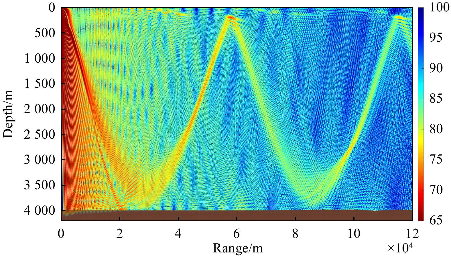
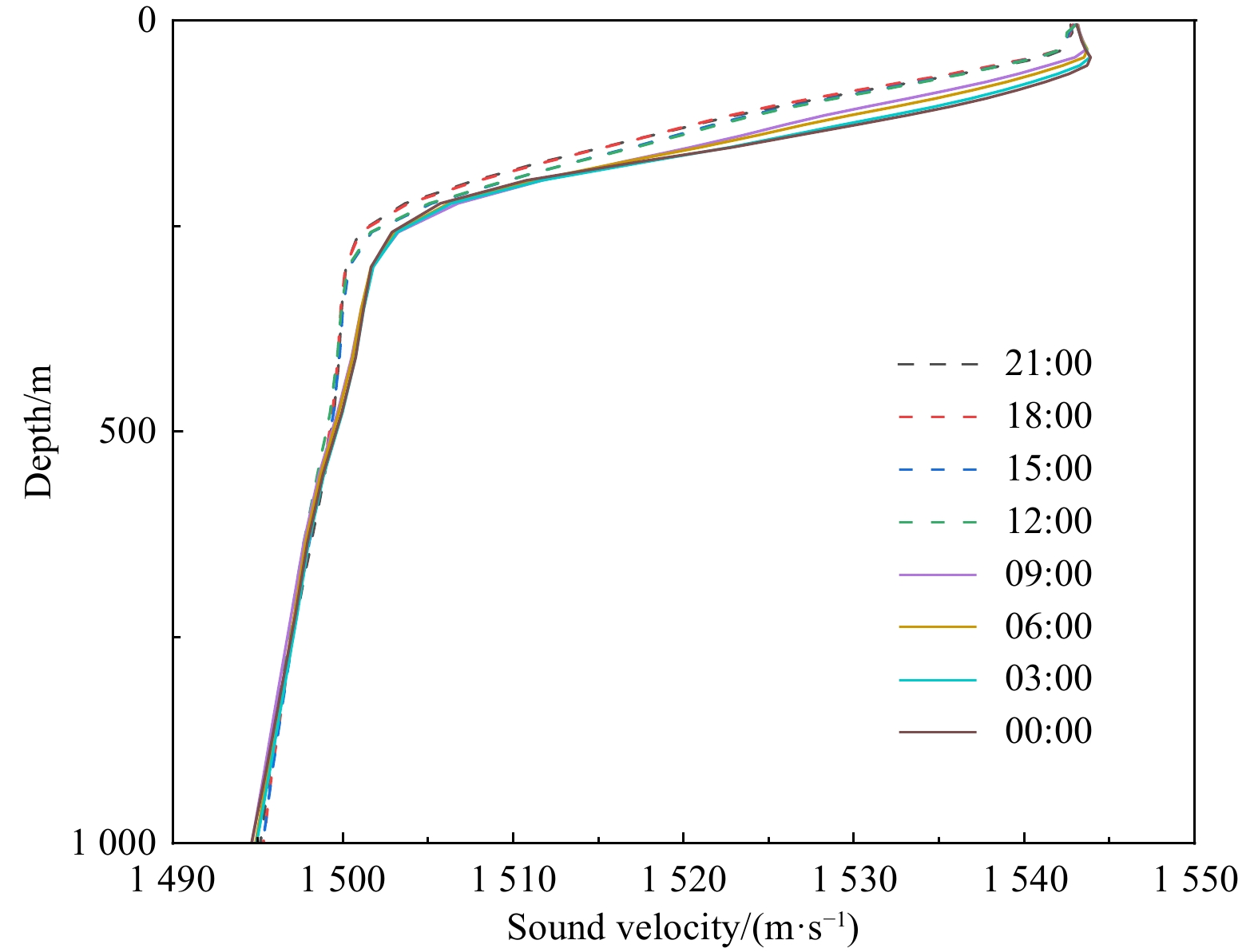
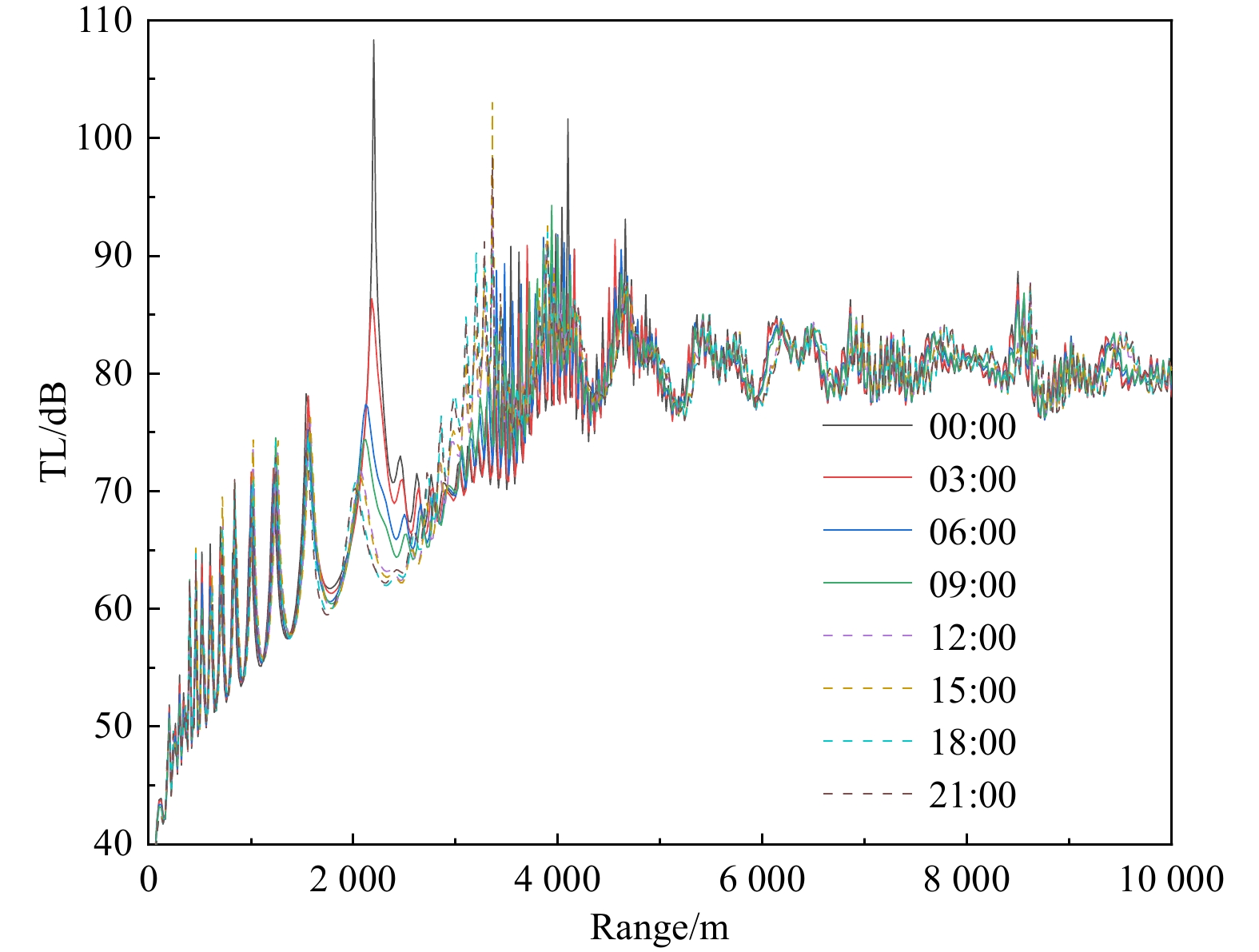
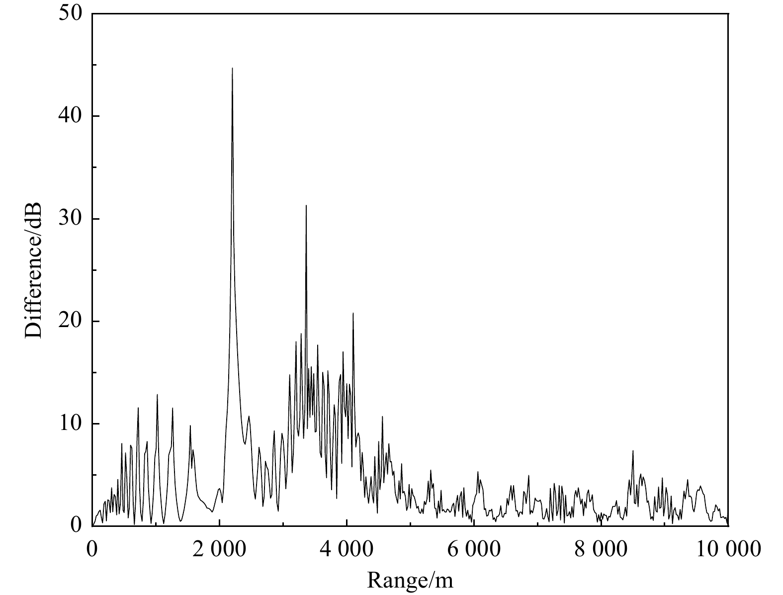
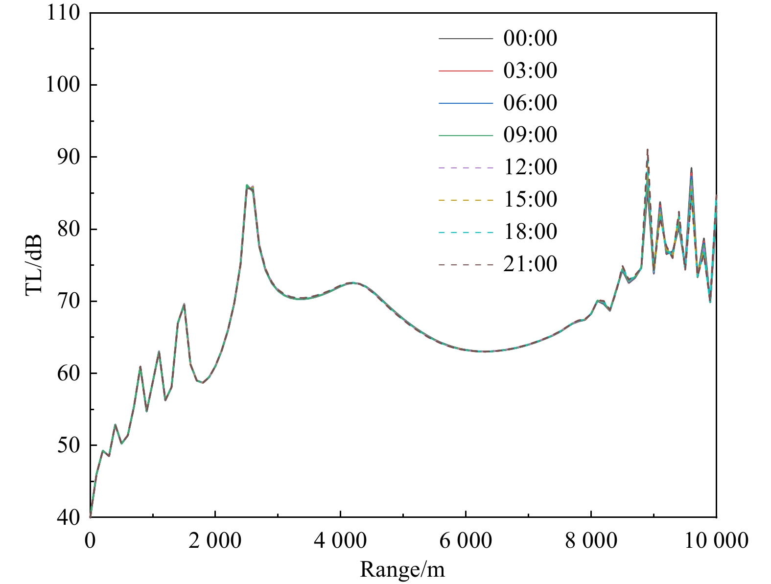
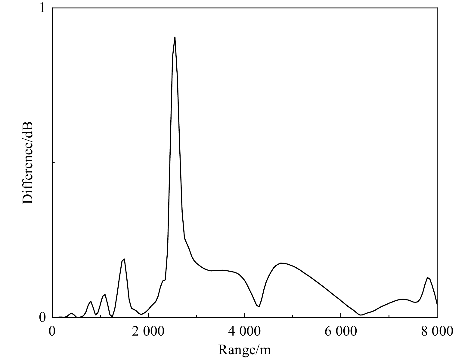
Figure 29 shows the acoustic propagation loss at noon at Point C in the South China Sea. Figure 30 depicts the sound speed profile every three hours over a day. Figure 31 illustrates the near-field (10 km) acoustic propagation loss at different times, while Figure 32 displays the difference between the maximum and minimum values of acoustic propagation loss each day at various distances. Combining Figures 29 and 30 reveals that this area exhibits typical characteristics of deep-sea sound channels, with the first convergence zone located approximately 50 km away and the second convergence zone approximately 105 km. The sound speed profile, as indicated in Figure 30, shows relatively consistent trends throughout the day, with slight variations. From the afternoon to night, the sound speed values below 100 m are slightly lower than those in the morning; at 15:00, the sea surface temperature rises, resulting in an increase in the sea surface sound speed. Figure 31 presents the near-field acoustic propagation loss at a reception depth of 200 m at this point, which increases with horizontal distance and exhibits fluctuating changes. The variations at different times during the day are more pronounced, with peak values reaching up to 18 dB. Between

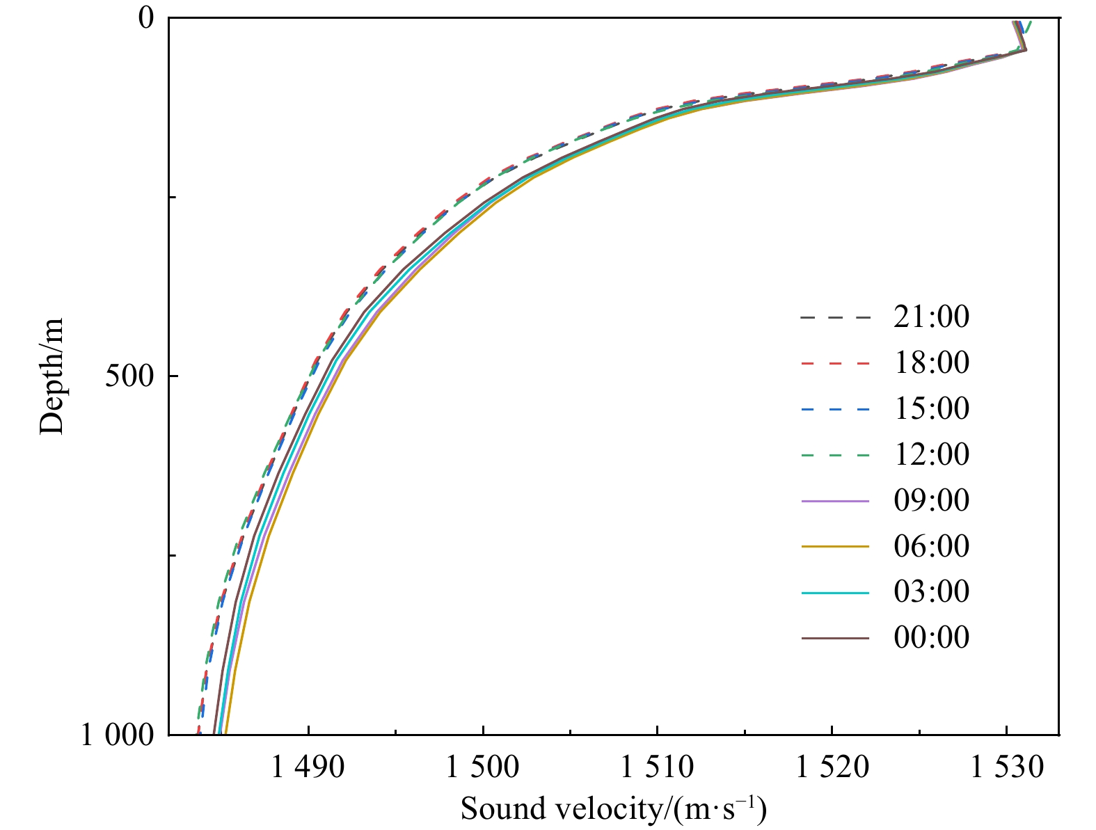
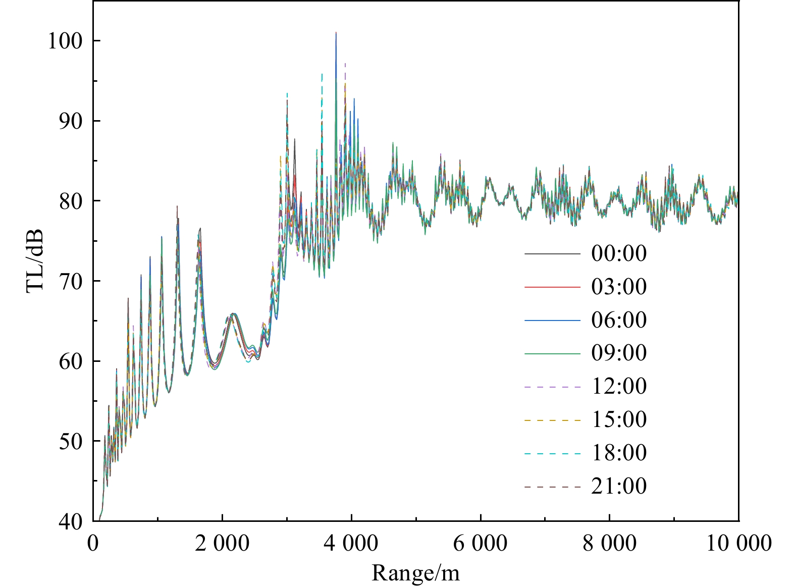
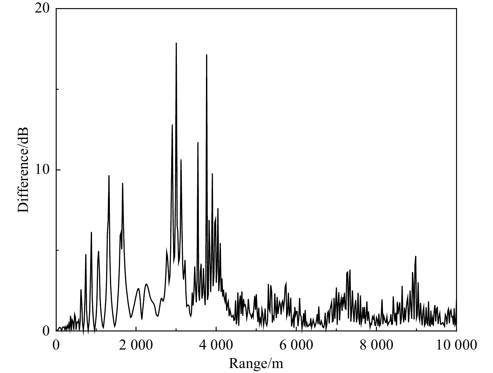
Figure 33 shows the sound propagation loss at Point D in the Indian Ocean. Figure 34 displays the sound speed profile at different times at Point D. Figure 35 represents the near-field (10 km) sound propagation loss at different times. Figure 36 illustrates the variation of the difference between the maximum and minimum values of sound propagation loss with horizontal distance. Similar to Point C, the designated area in the Indian Ocean also exhibits deep sound channel characteristics, with the first convergence zone located approximately 60 km away and the second convergence zone approximately 120 km away from the source. Compared to Point C, the sound speed profile at Point D has a stronger sound layering effect, and the overall sound speed is higher. This is reflected in Figure 33, in which the position of the convergence zone clearly shifts away from the direction of the sound source. In a comparison of sound speed profiles at different times throughout the day, it can be observed that the sound speed values are slightly lower from the afternoon until the night, and this variation is evident even at the sea surface. In Figure 35, the overall trend of sound propagation loss shows an initial increase followed by a stable period. Between
Compared to Points C and D, Point F exhibits a positive gradient distribution in the sound speed profile, as shown in Figure 38. Point F does not have a deep-sea sound channel; when sound waves enter the deep isothermal layer, they quickly deflect downwards and cannot form an effective sound propagation path, leading to the inability of acoustic energy to converge. As indicated in Figure 37, Point F possesses a typical sea surface sound channel. Due to the lower sound speed at the sea surface, incident sound waves are deflected towards the sea surface, reflect off it, and continue propagating forward after reflection, creating a sea surface sound channel through repeated deflections and reflections. According to Figure 39, the overall trend of sound propagation loss at Point F is similar to Points C and D, with an initial increase followed by a stable period. However, the energy fluctuation frequency at Point F is smaller, with a narrower range. In this region, there are no significant daily variations observed in both the sound speed profile and sound propagation loss at Point F. The difference between the maximum and minimum values of sound propagation loss remains within 1 dB, with most positions showing less than a 0.2 dB difference, which is negligible compared to Points C and D. The lack of distinct daily variations in sound propagation at Point F may be attributed to the fact that the Arctic Ocean region is in a polar night state in January, with very low solar radiation intensity. Therefore, the daily variation characteristics of various oceanic elements observed at mid-low latitudes are not evident at Point F, resulting in the absence of notable daily changes in sound propagation.
This section provides a brief exploration of the diurnal variations in sound propagation in three typical marine areas, obtaining preliminary insights into the diurnal variations in sound speed profiles and the corresponding changes in the acoustic environment. Different marine areas exhibit slightly different characteristics of variation, influenced by factors such as geographical location. The primary reason for these differences is likely the impact of solar radiation changes during the day and night on seawater temperature, which in turn affects the sound speed of seawater and consequently influences the characteristics of sound propagation in seawater.
This study conducts a series of acoustic analyses and application studies on the new generation of high-resolution ocean reanalysis product CORA v2.0 in China.
In a comparison of temporal data, CORA v2.0 data have a relatively small overall average offset compared to Argo data, both remaining within ±2 m/s, with a root mean square error of less than 3 m/s. The consistency between the two datasets is best in the Indian Ocean. In a comparison analysis of monthly average data, the relative error of CORA v2.0 data compared to WOA and GDEM data shows significant variations with depth and month. At the depth level, in the upper ocean region above 500 meters, CORA v2.0 data show more noticeable deviations from the reference data, with maximum absolute values reaching 16 m/s. At an approximately 2000-m depth, there is a water layer where the difference in sound speed between CORA v2.0 and reference data differs from the upper and lower layers, showing negative values, indicating that the sound speed value of CORA v2.0 is lower than the reference dataset. In terms of time, in shallow sea areas during summer, the difference between CORA v2.0 data and the two reference datasets is often greater than 0, while it tends to decrease in winter. Deep water, being less affected by seasonal variations, does not show a clear annual change pattern. The average deviation and root mean square error between datasets in the western Pacific Ocean and Arctic Ocean are relatively small, mostly within ±1 m/s. Overall, the consistency between CORA v2.0 data and Argo data is the best, while CORA v2.0 data and GDEM and WOA data show a consistent bias in spatiotemporal distribution. Compared to GDEM data, the consistency of CORA v2.0 data with WOA is higher in most cases.
The global distribution of seawater sound speed exhibits distinct spatial and temporal characteristics. Spatially, the global sound speed distribution forms bands in subsurface seas, with sound speed decreasing with increasing latitude; in deep-sea areas, the differences in sound speed are relatively small across different regions globally. Sound speed values in different regions vary due to factors such as ocean currents, topography, or other factors, with polar regions typically showing positive sound speed gradients in sound speed profiles. Temporally, sound speed variations in shallow sea areas are more pronounced compared to deep-sea areas, with surface waters showing significant seasonal variations. Sound speed changes exhibit some lag as depth increases, and beyond a certain depth, they no longer show temporal variability. Sound speed variations are greater in mid- to low-latitude regions compared to polar regions. In mid-latitude or monsoon regions, seasonal variations in seawater sound speed profiles are distinct.
In the exploratory analysis of the application of CORA v2.0 data with a 3-hour temporal resolution, it was observed that the diurnal variation of the underwater sound field is not very prominent. However, overall, from the afternoon to night, sound speed values are slightly lower than in the morning. There are significant differences in underwater sound propagation losses at different times of the day, ranging from a 2000 to
Through preliminary research, CORA v2.0 data, as a new generation of high-resolution ocean reanalysis product in China, demonstrates high reliability and significant utility in marine acoustics research.

Supported by:
Beijing Renhe Information Technology Co. Ltd

Tao Shiyuan, Yu Yi, Xiao Wenbin, Zhang Weimin, Zhao Yanlai. Analysis of the distribution of sound velocity profiles and sound propagation laws based on a global high-resolution ocean reanalysis product[J]. Acta Oceanologica Sinica.

| Point | Depth/m | Position |
| A | 11.55°N, 130.95°E | |
| B | 39.55°S, 147.35°W | |
| C | 18.15°N, 117.95°E | |
| D | 5.25°N, 86.05°E | |
| E | 150.8 | 11.65°N, 43.55°E |
| F | 75.45°N, 144.05°W |
DownLoad:
CSV
| Moment | 2014-01-28 21:00 | 2014-02-07 21:00 | 2014-04-30 03:00 |
| ME | − |
− |
|
| RMSE |
DownLoad:
CSV
| Moment | 2014-05-11 21:00 | 2014-11-22 21:00 | 2014-12-04 21:00 |
| ME | − |
− |
− |
| RMSE |
DownLoad:
CSV
| Moment | 2014-01-30 18:00 | 2014-06-14 21:00 | 2014-06-19 18:00 |
| ME | − |
||
| RMSE |
DownLoad:
CSV
| Point | Depth/m | Position |
| A | 11.55°N, 130.95°E | |
| B | 39.55°S, 147.35°W | |
| C | 18.15°N, 117.95°E | |
| D | 5.25°N, 86.05°E | |
| E | 150.8 | 11.65°N, 43.55°E |
| F | 75.45°N, 144.05°W |
| Moment | 2014-01-28 21:00 | 2014-02-07 21:00 | 2014-04-30 03:00 |
| ME | − |
− |
|
| RMSE |
| Moment | 2014-05-11 21:00 | 2014-11-22 21:00 | 2014-12-04 21:00 |
| ME | − |
− |
− |
| RMSE |
| Moment | 2014-01-30 18:00 | 2014-06-14 21:00 | 2014-06-19 18:00 |
| ME | − |
||
| RMSE |
 DownLoad:


