A synthetic autonomous profiling float array in a Lagrangian particle tracking system

1. Introduction

Since the launch of the International Argo Program (Array for Real-time Geostrophic Oceanography, Argo) in 2000, more than 17 000 autonomous profiling floats have been deployed in the global ocean by over 30 coastal countries and regions, maintaining an observational network composed of about 4 000 active floats. Over the past two decades, this observational network has accumulated more than 2.5 million profiles of temperature and salinity from 0 m to 2000 m depth, and has become an important data source for operational oceanography and atmospheric-ocean research (Roemmich et al., 1998, 2009; Roemmich and Gilson, 2009; Claustre et al., 2020; Liu et al., 2021; Chen et al., 2022), and is currently the most effective means of obtaining upper ocean data on a global scale. At the same time, Argo is also an important part of the Global Ocean Observing System (GOOS). Currently, the international Argo program is expanding from “core Argo” to “global Argo” (i.e., to seasonal ice-covered regions, the equator, marginal seas, western boundary currents, and water depths below 2000 m, as well as biogeochemical fields, etc.), with the goal of establishing a truly global, comprehensive observation network covering all water depths and multiple disciplines (Roemmich et al., 1998, 2009; Roemmich and Gilson, 2009; Chai et al., 2020).

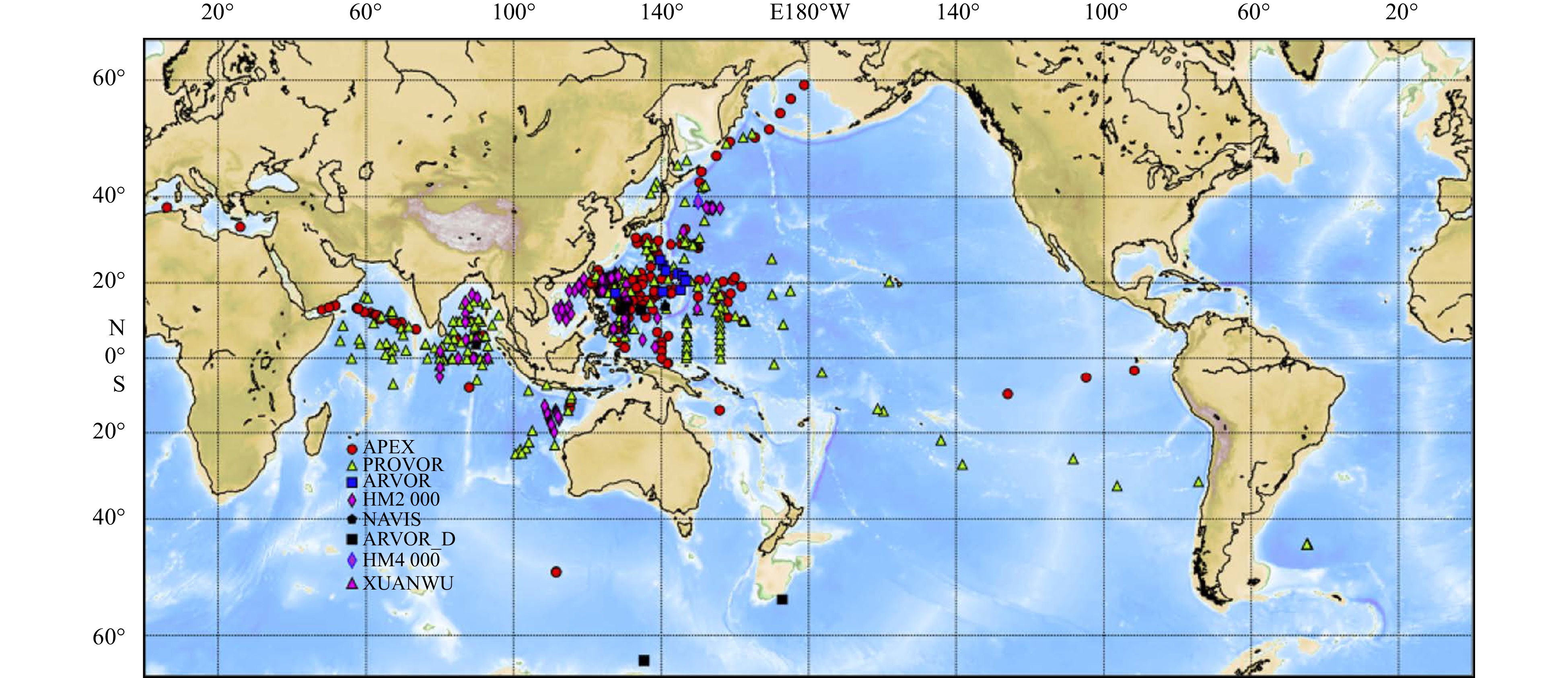
As an important member of the Argo program, China has also made great efforts to construct the Argo observation network (Liu et al., 2023). As of October 2023, China’s Argo program has deployed over 500 new types of autonomous profiling floats in the key oceanic regions (the western Pacific Ocean, the South China Sea, and the North Indian Ocean, see Fig. 1). There are still many challenges to be overcome in the process of aligning China’s profiling floats with the International Argo Program. For example, the data from profiling floats are not openly accessible until the sharing rules are fully established, which appears to be in conflict with the provisions and requirements outlined in the standard resolution (i.e., Data-sharing Resolution XX-6 on the Argo Project) or guidelines (guidelines for the implementation of resolution XX-6). In order to address this issue, several Chinese ocean research institutes, under the guidance of the Second Institute of Oceanography, Ministry of Natural Resources, collaborated on drafting the Resolution of Chinese Argo project (published in Chinese). The goal of this project is to promptly incorporate Chinese profiling floats into the international Argo program, making the data can be used by scientists globally.

Figure  1.  Launch positions of all China profiling floats since 2002. By February 7th, 2023, a total of 550 China profiling floats have been deployed. The different markers indicate the various types of floats (access from China Argo Real-time Data Center, http://www.Argo.org.cn).

DownLoad: Full-Size Img PowerPoint

Another challenge comes from designing float arrays. Due to the free drift of the profiling floats after deployment, some oceanic regions tend to be over-concentrated with floats, while some regions have observational gaps, making it difficult to effectively cover a larger area and make full use of the limited float resources. Therefore, it is of great scientific significance to optimize the deployment locations of the floats so that the distribution of the floats in the global Argo observation network is uniform. In addition, unlike the international Argo floats that use the ARGOS and Iridium satellite communication systems, the domestically produced autonomous profiling floats deployed by China mainly use the Beidou satellite for data transmission (BD float hereafter). The Beidou-2 permits the data transmission (short message) in the nominal range of 5°–55°N and 70°–140°E. According to the observations received from the BD floats, the coverage of Beidou-2’s short message presents a semi-elliptical distribution (Montenbruck et al., 2013; Li et al., 2019; Nie et al., 2020). The higher the latitude, the wider the coverage, while the lower the latitude, the narrower the coverage. At higher latitudes (i.e. the latitude of Kuroshio Extension), the signal coverage can reach 160°E, while at lower latitudes (around 5°N), the eastern boundary of Beidou communication can only reach its nominal 140°E. The loss of contact due to drifting out of the Beidou coverage area is thus an important issue to be considered when deploying BD floats. Therefore, it is crucial to formulate and optimize the deployment strategies for the construction of a BD float network across the Pacific Ocean, South China Sea, and northeastern Indian Ocean, while the related theoretical work is still relatively scarce.

This study aims to use a numerical model to investigate the representativeness and predictability of profiling float observation. We use an eddy-resolved hydrostatic version of the Estimating the Circulation and Climate of the Ocean, Phase Ⅱ (ECCO2) model (available at http://ecco2.org/; see Menemenlis et al., 2005) for our research domain. We simulate the BD float behavior with a Lagrangian float-tracking model and the model output fields. By deploying a large number of floats within the model, we construct probability density functions (PDFs) of the simulated-float trajectory end points. We evaluate the performance of the simulated floats by comparing them with core Argo trajectories, which allow for a statistical ensemble approach. These statistics can help optimize the float deployment station design, reducing the chance of drifting into shallow seas (such as the East China Sea) and out of the coverage of the Beidou satellite communication, thus ensuring the normal working life of the BD floats.

The paper is organized as follows: Section 2 introduces the Argo simulation system, including the ECCO2 dataset, the Lagrangian particle tracking model, and a subgrid-scale parameterization process for the simulated profiling floats. Section 3 presents results from the Argo simulation system, with a focus on the PDFs of float displacements. Within our study area, we simulate float trajectories in different subdomains to calculate the probability of floats escaping from the Beidou-2’s short message coverage range at different latitudes, and find maintenance recommendations of the Pacific−South China Sea−Indian Ocean float array. Finally, Section 4 summarizes the results and assesses shortcomings of float simulations in regions with strong background velocities or with numerous eddies. We also identify priorities for further improvements.

2. Method and datasets

2.1 Modeled frame of Argo observation

We focus on a joint region of Northeast Indian Ocean−South China Sea−Northwest Pacific Ocean (0°–40°N, 70°–140°E; see Fig. 2), where profiling floats have been deployed more than 500 since the last two decades (Liu et al., 2023). The local circulations in this region are complex and variable. Multiple equatorial currents and western boundary currents play key roles in the latitudinal and longitudinal heat, mass transport and the exchange process between Pacific−Indian Ocean basins and hemispheres, directly affecting and modulating the variation of the intersection area and local ocean-atmosphere interactions. Besides, the above region directly links the four gyres of the Indo−Pacific low-latitude basin, including the North Pacific Tropical Gyre (NPTG; Wijffels et al., 1998), the South Pacific Tropical Gyre (SPTG; Roemmich et al., 2007), the South China Sea Gyre (SCSG; Shaw et al., 1999; Liu et al., 2008), and the Indian Ocean Tropical Gyre (IOTG; Du et al., 2019; Wu et al., 2020).

Figure  2.  Bottom topography of East Indian-South China Sea-Northwest Pacific Ocean from the ECCO2 model. The 2000-m isobaths are marked by yellow solid lines. Blue dashed line box represents nominal coverage of Beidou-2 satellite’s short message. Three subdomains are marked (colored solid lines) as the releasing regions of the simulated profiling floats in the following sections. Four main gyres of the Indo-Pacific low-latitude basin are marked by black lines with arrows. NPTG: North Pacific Tropical Gyre; NPSG: North Pacific Sea Gyre; SPTG: South Pacific Tropical Gyre; SCSG: South China Sea Gyre. SMC: Southeast Monsoon Current; NMC: Northeast Monsoon Current.

DownLoad: Full-Size Img PowerPoint

To simulate mesoscale motions of profiling floats within the region, we use ECCO2 velocity field (available at http://ecco2.org/; see Menemenlis et al., 2005) configured for the Pacific Ocean-the South China Sea-North Indian Ocean. ECCO2 is an assimilating version of the MIT General Circulation Model (MITgcm). We use the “Cube 92” solution, which is run on a “cubed sphere” with 18-km (eddy permitting) horizontal grid spacing and 50 vertical levels unevenly distributed between the surface and 6000 m (Menemenlis et al., 2008). ECCO2 was optimized via Green’s function methodology (Menemenlis et al., 2005) to best represent observed hydrography. ECCO2 fields do not resolve high-frequency or high-wavenumber dynamics, and simulated floats will not be influenced by processes that ECCO2 does not resolve. For the analysis, we use archived 3-day average ECCO2 fields that have been interpolated to a regular 0.25° × 0.25° grid.

The comparison of ECCO2 sea surface height (SSH) field to the AVISO-mapped satellite altimetry product gives a qualitative assessment of the surface circulation and its variability during the float simulation period (January 1, 2015 to December 31, 2022). As an example of the South China Sea and the West Pacific, the mean sea surface height of the inner region of the South China Sea and the Luzon Strait depicted by the ECCO2 model is basically consistent with the observation from the AVISO satellite (as shown in Figs 3a and b), which is characterized by low values in the northern part of the South China Sea and high values in the outer sea of the Luzon Strait, with a value of about 1.1 m. The variance of SSH anomaly also reflects the consistency between ECCO2 and AVISO observations, with the maximum value (about 0.2 m) appearing in the middle of the South China Sea and the Kuroshio pathway. In addition, the vertical dynamic process depicted by the ECCO2 model is also close to the observation. Taking the vertical temperature and salinity change characteristics of the Luzon Strait as an example, both the ECCO2 model and Argo profile observation can depict the intrusion process of the Kuroshio water (Figures not shown), and the core of the intrusion of the high-salinity Kuroshio water is 100–200 m, which is consistent with the basic observational facts. The standard deviation (STD) of the two SSH products shows a similar structure (Figs 3c and d). High variance occurs in the middle of South China Sea, the Kuroshio pathway. Like the mean, the structure is patchy as a result of the relative brevity of the time series. Despite variability differences at specific locations, both the model and the AVISO product have roughly equal levels of SSH variability.

Figure  3.  Mean SSH (m) during 2015−2022 from the AVISO-mapped product (a) and ECCO2 dataset (b), and the standard deviation (STD) of SSH from the AVISO-mapped product (c) and the ECCO2 model (d).

DownLoad: Full-Size Img PowerPoint

2.2 Lagrangian particle tracking model

Float trajectories are simulated using an Argo module of the offline particle tracking model Octopus (http://github.com/jinbow/Octopus/; see e.g., Tamsitt et al., 2017; van Sebille et al., 2018; Wang et al., 2018, 2020, 2021). The model integrates float trajectories using daily average horizontal velocities from the (1/4)°–resolution model and vertical velocities derived from real Argo floats. Float trajectories are integrated via a Lagrangian advection scheme: $ {{\partial {{\boldsymbol{X}}_{\boldsymbol{i}}}} /{\partial t}}{{ = }}{{\boldsymbol{V}}_{\boldsymbol{i}}} $, where X_i is the (vector) position of the i-th particle, t is the time and V_i is the velocity vector mapped to the numerical float position using three-dimensional linear interpolation. In addition to the model velocities, Octopus Lagrangian tracking model also includes a stochastic velocity component to account for the float displacement caused by processes (such as turbulence) that are unresolved by the ECCO2 model. The subgrid-scale processes are parameterized by $ {{\Delta }}{{\boldsymbol{X}}_{{i}}} = \sqrt {2{\boldsymbol{K}}\delta t}\; \omega (t) $, where K represents the diffusivity tensor $ ({K_x},{K_y},{K_z}) $, $ \omega $ represents a Wiener process (stochastic random walk displacements) with unit variance, and $ \delta t $ denotes the time step for the Lagrangian integration (e.g., van Sebille et al., 2018). The particle trajectory in discrete form becomes

where n represents the time step number. In practice, the random number generator should be carefully chosen, because not all numbers are suitable for use in random walk models (Hunter et al., 1993). Here we implement the normal random number generator algorithm described by Kinderman and Monahan (1977), with a horizontal diffusivity of 1 m²/s, which is consistent with the diffusivities of the ECCO2 dataset.

2.3 Simulated float parameters and deployment scheme

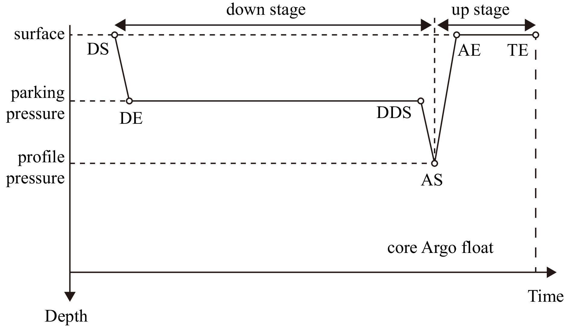
Simulated profiling floats are configured to follow the same cycle as the real Argo floats, as defined in Fig. 4, including an initial descent to 1 000 m, parking time at 1 000 m, a further descent to 2 000 m, then ascent from 2 000 m depth to the surface, and finally an interval of time at the ocean surface to transmit data via satellite. For the period from 2015 to 2022, cycle timings for the delayed-mode BD float data were obtained from the observation and research station of global ocean Argo system (Hangzhou) (ftp://ftp.argo.org.cn/pub/ARGO/china/) within the research basin. Ocean currents are nonuniform in the vertical, which affects the true trajectories and how we interpret float displacements.

Figure  4.  Schematic of one float cycle for a core Argo float, which includes descent, parking, deep profiling, and surface telemetry. The schematic map indicates the times when descent starts (DS), descent ends (DE), deep descent starts (DDS), ascent starts (AS), ascent ends (AE), and transmission ends (TE). The definitions are adopted from Ollitrault and Rannou (2013).

DownLoad: Full-Size Img PowerPoint

Simulation of profiling floats (parking at 1 000 m depth) trajectory requires parameterization of Argo based on observation data, including Argo working cycle time, vertical ascent/descent rate and float deployment scheme (including deployment position, scale and deployment time of virtual floats). By taking each variable as the initial condition of virtual floats, the Lagrangian tracking algorithm can be used to calculate and output the three-dimensional position of virtual float in the background model flow field. The Argo parameters configured in this work are shown in Fig. 4, including surface drifting, descending, parking, ascending and surface stages. In the simulation, the time of each stage is selected according to Table 1, and the single working cycle is about 5 d. All the Argo clock schedules are configured to approximate an “average” float, with cycle times and parking depths representing the weighted average of cycle times.

Table  1.  BD float clocks configured in the BD float simulation

BD float stage	Simulated BD float clock/h
Descent stage	5.4
Parking stage	102.2
Deep descent stage	5.4
Ascend stage	6.5
Surface stage	0.5

 | Show Table

DownLoad: CSV

In December 2020, China designed a special project from which about 500 profiling floats were deployed across the Northwest Pacific, South China Sea, and the Indian Ocean. The majority of these floats were equipped with a communication system covered by Beidou-2 satellites. In order to optimize the float deployment position design, to avoid the float drifting into shallow waters (such as East China Sea) and out of the coverage of Beidou-2 satellite short message, and to ensure the normal working life of the whole fleet, four deployment experiments have been carried out in this work (see the details in Table 2). To maximize the statistical samples using a model of limited duration, we carry out repeated simulated-float releases, separated by time intervals large enough to produce statistically independent trajectories. The autocorrelations of mid-layer velocities (corresponding to core Argo floats) imply that the decorrelation time scales are about 5 d (Wang et al., 2018). The simulated floats are thus released at 30-day intervals starting on Day 1, and with the last release on Day 2791. Thus, there are at most 94 independent release times during the 8-year (January 1, 2015 to December 31, 2022) of the model run for each releasing experiments.

Table  2.  Description of the profiling float simulation experiments

Experiment	Releasing position	Releasing time	Simulation duration/d	Releasing grid	Quantity of single release	Repeat releasing time
Exp_1	East of the Luzon Strait (20°–28°N, 122°–127°E)	August 1 of each year	300	0.5° × 0.4°	100	8
Exp_2	Philippine Sea (8°–25°N, 127°–135°E)	August 1 of each year	300 & 400	0.8° × 1.7°	100	8
Exp_3	Bay of Bengal (6°–12°N, 83°–90°E)	the first day of every month	400	0.7° × 0.6°	100	94
Exp_4	East Indian–South China Sea– Northwest Pacific Ocean (0°–40°N, 70°–140°E)	the first day of January, April, July, and October of each year	720	1.5° × 1.5°	823	23
Exp_5	Kuroshio Extension & monsoon current of Bay of Bengal	August 1 of 2005	100	0.1° × 0.1°	7700 & 15600	1

 | Show Table

DownLoad: CSV

3. Results

3.1 Float simulation in the east of the Luzon Strait

The marginal seas of China (including the Bohai Sea, Yellow Sea, East China Sea, and South China Sea) are all affected by the Kuroshio and its branches. The range of Kuroshio intrusion into the East China Sea shelf in different seasons is different, and it has obvious seasonal characteristics. Although the Kuroshio water constitutes a transport channel for material from east of the Luzon Strait to the East China Sea, the shallow water depth of the East China Sea (as shown in Fig. 2) hinders the entry of profiling floats which drift in the middle layer (1000 m). However, historically, some floats deployed east of the Luzon Strait and Taiwan Island (20°–28°N, 122°–127°E) had entered the East China Sea following Kuroshio and beached on the continental shelf. Therefore, the possibility of floats released east of the Luzon Strait drifting into the East China Sea should be investigated. In this section, the deployment region of the simulated floats is 20°–28°N, 122°–127°E, (as shown in Fig. 2, also see Table 2), and the grid setting is 0.5° × 0.4° with a single deployment of 100 floats. We select the floats deployed in August of each year in the overall simulation experiment (the deployment time of floats in the observational condition is August 2021), and the total number of deployments is 8 times.

Simulation results showed that under the influence of the South China Sea summer circulations and Kuroshio, the overall flow direction of simulated float trajectories deployed in August in recent years is northeastward (shown in Fig. 5). The number of simulated floats entering the East China Sea is very small (only 3 from 800), and the spilling effect is not significant, so it can be expected that the floats deployed in Luzon Strait will only have a small probability of entering the East China Sea under the influence of the ambient currents, which is consistent with theoretical deduction.

Figure  5.  Lagrangian trajectories for simulated floats during 300-d model runs. All the floats were initially released in the east of the Luzon Strait (20°–28°N, 122°–127°E). The black dots denote the releasing positions. The details of the simulation can be referenced in the description of Exp_1 in Table 2.

DownLoad: Full-Size Img PowerPoint

It should be noted that the above conclusions rely on the accuracy of the float simulation system and the model flow field (ECCO2). Due to the relatively poor simulation performance of ECCO2 in the nearshore area, discrepancies between the simulated float trajectories with observations may occur. In addition, a random motion module is an important component in the Octopus Lagrangian tracking model, which the subgrid random motion is used to present the mixing process caused by Brownian motion ($ {{\Delta }}{{\boldsymbol{X}}_{{i}}} = \sqrt {2{\boldsymbol{K}}\delta t}\; \omega (t) $, see details in Section 2.2). In the model, the horizontal diffusion coefficient (K) determines the strength of random motion, with the larger diffusion coefficient, the stronger the stochastic random walk displacements ($ { {\Delta {\boldsymbol{X}}}} $). In the float simulation system, the horizontal diffusivity coefficient is set to 1 m²/s, consistent with the background flow field. However, according to Batchelor (1952) theory, turbulent mixing leads to gradually separation of two adjacent fluid particles in the drifting process, which means that the random module would cause system uncertainty in the process of stepwise integration calculation of profiling floats position, and the uncertainty would increase with time. When the background flow field is added, this system uncertainty will be further amplified by the advection effect.

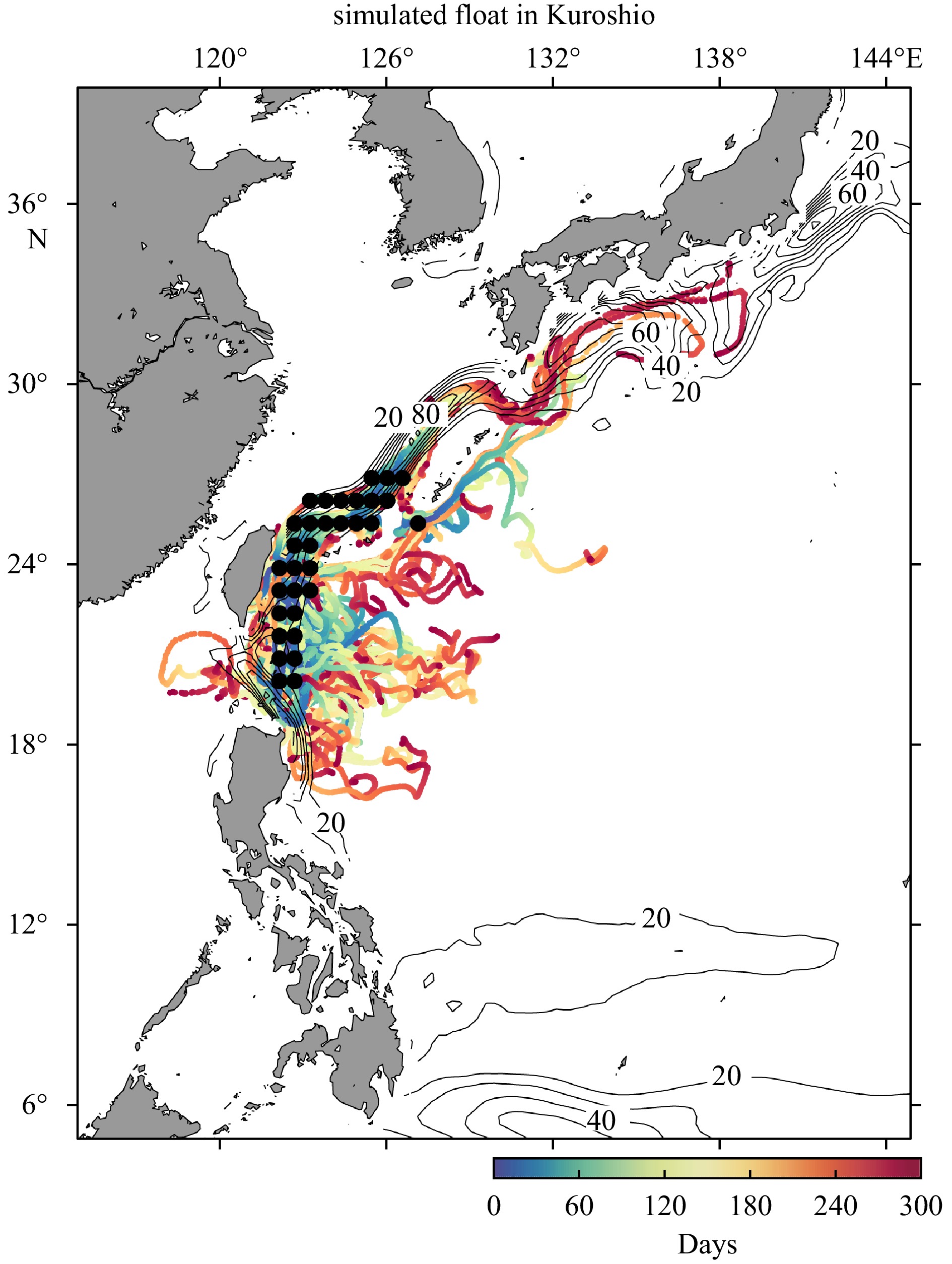
The Kuroshio is the main flow in this domain and worthy of further research. We thus select the floats trapped in the Kuroshio to assess its impact on their drift trajectory by analyzing statistical data. By analyzing the experimental results of Exp_1, we find a total of 32 sets of floats within the Kuroshio axis with a velocity exceeding 20 cm/s, which translates to 32 times 10 buoys. We select this part of the floats and mapped out their drift trajectories (shown in Fig. 6). During the simulation duration, approximately 2/3 (207) of the floats move northward along the strong front of the Kuroshio, while the remaining floats are trapped at the Luzon Strait. By calculating the drift distances of the floats, it is shown that the floats that remain on the Kuroshio axis have a significantly longer average drift distance, averaging 1090 km within 300 d, while the floats that are not on the Kuroshio axis have an average drift distance of only about 254 km within the same time period.

Figure  6.  Lagrangian trajectories for simulated floats during 300-d model runs. All the floats were initially released in Kuroshio axis (with the velocity beyond 20 cm/s). The black dots denote the releasing positions. The overlaid contour lines represent the geostrophic current velocity beyond 20 cm/s from the AVISO-mapped product with 20 cm/s interval.

DownLoad: Full-Size Img PowerPoint

3.2 Float simulation in the Philippine Sea

The Philippine Sea lies to the east and north of the Philippine Archipelago in the western North Pacific Ocean. The deepest part of the shelf is over 2500 m and it is the most important pathway for water and heat-salt exchange between the South China Sea and the western Pacific Ocean. When the Kuroshio flows northward along the Philippine Archipelago, passing the east side of the Luzon Strait, two typical paths of motion are often formed: one is a non-invasive direct crossing of the Luzon Strait to the north; the other is a westward intrusion to the South China Sea. Therefore, the complicated oceanic circulations in the Philippine Sea and the changes of west boundary currents of Pacific such as Kuroshio and Ryukyu currents at the Luzon Strait will have a strong influence on the float drifting in this area. This is manifested in the overall clockwise motion of the floats under the influence of the subtropical gyre in the North Pacific, as well as the intrusion of the Kuroshio into the South China Sea caused by meso-scale processes and to a certain extent, the intrusion of some floats into the East China Sea. Based on the simulation in Section 3.1, the releasing boundary was expanded to the Philippine Sea (8°–25°N, 127°–135°E), the simulated trajectory time length extended to 400 d (see more details in Table 2). The aim of this section is to discuss the drifting characteristics of float drifting in the Philippine Sea under the influence of Kuroshio and Ryukyu currents. Meanwhile, the coverage range of Beidou Satellite is proposed to be 5°–55°N and 70°–140°E. We will discuss the approximate time and location that simulated floats, which are operating in the Philippine Sea, drift out of the Beidou coverage range.

As illustrated by the simulation results in Figs 7 and 8, with the advection of the Philippine Ocean currents, some floats released in August of each year can drift off Beidou coverage range through the eastern and southern boundaries. For example, in the 300 d simulation (Exp_2; see details in Table 2), out of the total 800 floats (100 floats × 8 groups), approximately 36 floats crossed out from the eastern boundary of Beidou coverage with a ratio of 4.5%. During the statistics calculation, if the float first breaches the eastern boundary during its operation, we will consider it to have drifted out of the Beidou coverage region and include it in the statistics. These floats mostly concentrated between 7°–21°N and were transported by the eastward zonal jets of the North Pacific (Xia and Du, 2022). The number of floats crossing out from the southern boundary of the Beidou coverage is much smaller, only 13 floats, with a ratio of 1.6%. This is due to the significant northward transport of Kuroshio, which largely prevents the floats from drifting southward. The floats crossing out from the southern boundary may be attributed to the presence of southward compensation currents such as the Mindanao Current, as well as mesoscale processes or diffusion processes. When the simulation was extended to 400 d, the results showed that more floats crossed out from both the eastern and southern boundaries of the Beidou coverage, with the number (ratio) reaching 64 (8%) and 21 (2.6%) respectively. In particular, in the 400-d simulation experiment, floats that are located on the Kuroshio Path will drift out of the Beidou coverage through the east boundary with the transport of Kuroshio Extension (KE) in the latitude range of 30°–34°N. This indicates that, in addition to considering the battery life limitation of the floats, the influence of KE on the float drifts should be taken into account to make sure the floats can operate in the Philippine Sea for more than one year. Therefore, it is suggested to avoid the strong frontal positions of Kuroshio and KE during deployment.

Figure  7.  Lagrangian trajectories for simulated floats during 300-d model runs (a), the statistics (as a function of latitude) for the floats exiting the Beidou coverage through the eastern boundary (b) and the statistics (as a function of longitude) for the floats exiting the Beidou coverage through the southern boundary (c). All the floats were initially released in Philippine Sea (8°–25°N, 127°–135°E). The black dots in a denote the releasing positions. Details can be referenced in the Exp_2 of Table 2. The number of floats drifting out of the Beidou Ⅱ short message coverage is calculated based on their final locations. Blue dashed line box in a represents theoretical coverage of Beidou Ⅱ short message.

DownLoad: Full-Size Img PowerPoint

Figure  8.  Lagrangian trajectories for simulated floats during 400-d model runs (a), the statistics (as a function of latitude) for the floats exiting the Beidou coverage through the eastern boundary (b) and the statistics (as a function of longitude) for the floats exiting the Beidou coverage through the southern boundary (c). All the floats were initially released in Philippine Sea (8°–25°N, 127°–135°E). The black dots in a denote the releasing positions. Details can be referenced in the Exp_2 of Table 2. The number of floats drifting out of the Beidou Ⅱ short message coverage is calculated based on their final locations. Blue dashed line box in a represents theoretical coverage of Beidou Ⅱ short message.

DownLoad: Full-Size Img PowerPoint

3.3 Float simulation in the Bay of Bengal

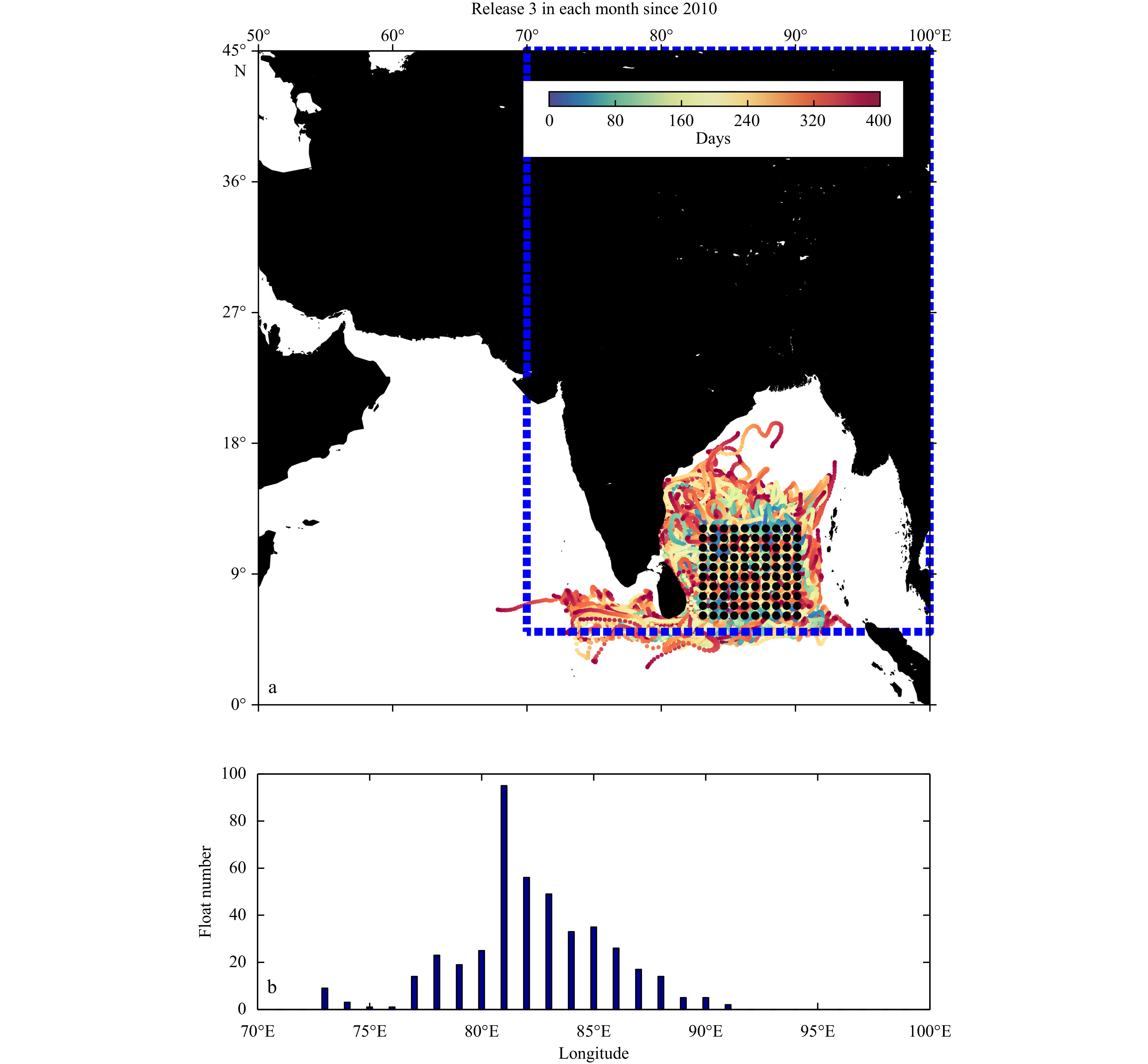
Under the strong seasonal gyre influences in the North Indian Ocean (e.g., Wyrtki, 1973; Swallow, 1984; Wu et al., 2020), there is a certain probability that the floats deployed in the eastern Sri Lanka will drift out of the Beidou coverage range, resulting in communication disconnection. This section is based on the outputs of Exp_3 (see Table 2), mainly discussing the drift trajectory of floats deployed in eastern Sri Lanka (6°–12°N, 83°–90°E) influenced by the North Indian Ocean circulation and the possibility of floats crossing the Beidou coverage area. The simulation results show that the floats deployed in the eastern Sri Lanka were mainly driven by the seasonal circulation of the Bay of Bengal, and most of the floats were still drifting in the Bay of Bengal within 400 d, while a small number of floats crossed the southern boundary of Beidou (as shown in Fig. 9). Due to the larger number of samples in Exp_3 (100 single deployments and 94 times of deployments), the number of floats crossing the southern boundary was much greater than the result of Exp_2. The statistical results show that the number of floats crossing the southern boundary is 743, accounting for 7.9% of the total samples (743/9400). The overall cross-border location of the floats is 73°–91°E, and the maximum probability cross-border location is approximately 81°E. It is inferred that the reason may be that the coastal current is strong due to Sri Lanka shore, resulting in a large amount of water transport, thus carrying more floats.

Figure  9.  Lagrangian trajectories for simulated floats during 300-d model runs (a) and the statistics (as a function of longitude) for the floats exiting the Beidou coverage through the southern boundary (b). All the floats were initially released in Bay of Bengal. The black dots in a denote the releasing positions. Details can be referenced in the Exp_3 of Table 2. Blue dashed line box in a represents theoretical coverage of Beidou Ⅱ short message.

DownLoad: Full-Size Img PowerPoint

3.4 A synthetic profiling float array over the joint oceans

In this section, the float trajectory simulation system is used to try deploying a synthetic profiling float array with a resolution of 1.5° × 1.5° in joint oceans, namely the East Indian−South China Sea−Northwest Pacific Ocean (5°–40°N, 70°–140°E). This region is generally similar to the location of the present China float network, and performing a preliminary analysis on its Lagrangian trajectories, exploring the effectiveness and the maintenance strategy of subsequent observation networks. In the simulation, the releasing position of the float array is selected in the open oceans with the water depth greater than 1500 m. The initial position of the array is on a 1.5° × 1.5° grid and contains a random deviation less than 1°, which is compared with observation conditions. To ensure an adequate sample size, the deployment strategy of synthetic float array is multiple deployment (totally 23 times), from 2015 to 2020, with an interval of three months (January, April, July, and October) to ensure that the derived float trajectories contain seasonal characteristics (see details in Table 2).

There are 823 effective floats deployment launched in the regions with the maximum depth over than 2000 m (see Table 2). In general, judging from the distribution of the float array, it can be inferred that during the floats’ life span of two years, the 1.5° × 1.5° float array can cover the entire Eastern Indian Ocean, South China Sea and Northwest Pacific region to realize real-time monitoring of the upper ocean in this region. In the North Pacific, the background circulation is stronger than that in other oceans, so the drifting of the floats is more intense and the trajectories are longer, leading to a sparser distribution of float array over time (Fig. 10). It can be inferred that when deploying floats in the North Pacific, the spatial resolution of float array should be increased. For other oceans (e.g., the South China Sea and the Bay of Bengal), due to the strong seasonal circulations, the temporal resolution of the array should be densified, that is, the time interval of floats releasing should be shortened.

Figure  10.  Distribution of the float locations of the 1.5° × 1.5° synthetic float array over the joint oceans within the model frame at different time. Panels a to d represent the results at Day 0, Day 90, Day 360, and Day 720, respectively. Blue dashed line box represents theoretical coverage of Beidou Ⅱ short message.

DownLoad: Full-Size Img PowerPoint

Optimization and maintenance of the float array in the western Pacific Ocean−South China Sea−North Indian Ocean should consider not only the working life of the battery (generally 2 years), but also the loss caused by the floats drifting out of the range of Beidou satellite short message coverage. According to the distribution of synthetic float array at different times under the model framework (as shown in Fig. 10), after 90 d of deployment, floats from the North Pacific began to drift out of the Beidou coverage area. At this time, the floats would be driven by the Kuroshio and North Pacific circulations to drift out of the eastern boundary of the Beidou coverage (in agreement with the conclusions of Section 3.1). The number of buoys drifting out from the North Pacific Ocean increases with time. Within 720 d after release, the floats can be driven as far as 165°E by the KE.

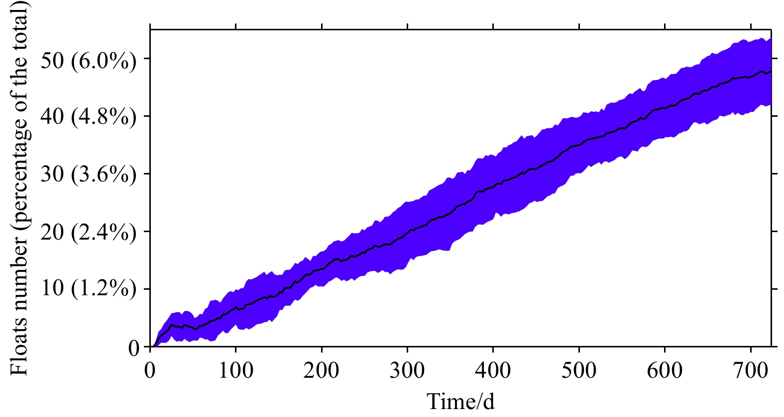
Statistics of floats drifting out of the Beidou range are displayed in Fig. 11. The number of floats drifting out of the Beidou coverage increases linearly over time, with approximately 2% (18 ± 3 of totaling 823) in 300 d and 5% (42 ± 6) in 720 d. Due to the limited deployment time of the simulated floats, system errors may contribute to a large level of uncertainty in these statistics. However, the present results suggest that, if losses due to floats drifting out of Beidou coverage are taken into account (not considering the battery power losses), roughly 20 additional floats must be added to the 1.5° float array in order to ensure effective observation during one year of operation, and around 42 buoys for a two-year period.

Figure  11.  Number of floats from the 1.5° × 1.5° synthetic float array drift out of the Beidou coverage as a function of modeled time period. The blue colored shading indicates the one standard deviation.

DownLoad: Full-Size Img PowerPoint

The overall spread of the float array is a function of the domain size and the flow structure. We quantify the horizontal spreading of the floats using a discretized two-dimensional probability density function (2D-PDF) denoted as $ P(x,y,T,\Delta L) $, where $ x $ and $ y $ indicate geographic coordinates, $ T $ represents the elapsed time, and $ \Delta L $ is the grid size. The 2D-PDF is computed by counting the number of floats within a grid box centered at $ (x,y) $ and normalizing by the total number of floats and grid box area $ {(\Delta L)^2} $ after spreading time $ T $. Thus, for example, $ P\;({x_0},{y_0},{\text{100\;d,}} {\text {1.5°}}) $ = 6 means that six floats can be found within a 1.5° × 1.5° grid box centered at$ ({x_0},{y_0}) $ at 100 d. The PDF of the float array at different times provides predictions of the float positions, indicating if the array is converging or diverging, with higher values indicating a higher likelihood of floats clustering at that position.

The results shown in Fig. 12 indicates that the relatively weak currents in the inner of the Bay of Bengal and the South China Sea, both semi-enclosed basins, result in high PDF values (around 20) at Day 180, Day 360 and Day 720 (23 deployments in total). This indicates that the floats deployed in these locations are not largely dispersed within two years, thus there is no need to supplement additional floats (not considering the power limit). We further analyze the simulation results and find the locations where the number of floats has significantly changed by comparing the numerical difference between the above PDFs, and consider the regions where the floats have obviously decreased as the locations that need to be supplemented for floats deployment in subsequent maintenance work. The result shown in Fig. 13 indicates that the cold colored patches of PDF (representing the net divergence of floats) are mainly distributed in the Philippine Sea. Due to its open shelf-sea boundary, the Philippine Sea is affected by strong western boundary currents, such as the Kuroshio, which leads to a decrease in PDF, indicating the higher dissipation rate of floats in this region, which is in agreement with that in Section 3.2. Therefore, the Philippine Sea should be considered as a priority area for replenishment of floats in the float array.

Figure  12.  PDF of the 1.5° × 1.5° synthetic float array over the joint oceans within the model frame at different time. a. Day 180; b. Day 360; c. Day 720. Blue dashed line box represents theoretical coverage of Beidou Ⅱ short message.

DownLoad: Full-Size Img PowerPoint

Figure  13.  PDF change of the 1.5° × 1.5° synthetic float array over the joint oceans within the model frame at different time (a. PDF at Day 360 minus that at Day 180; b. PDF at Day 720 minus that at Day 360). Blue dashed line box represents theoretical coverage of Beidou Ⅱ short message.

DownLoad: Full-Size Img PowerPoint

In addition, the positions where PDF changes greatly also exist in the boundary currents and monsoon currents. In the strong front system, floats are usually transported downstream very quickly due to the driving force of intense currents and result in accumulations. We select the Kuroshio Extension (32°–38°N, 138°–164°E) and the Bay of Bengal Monsoon region (5°–12°N, 82°–93°E) for an intensified single deployment of simulated floats (see Exp_5 in Table 2) and then calculate the PDF (x, y, 100 d, 0.1°) . Theoretically, the PDF is approximately equal to 1, the flow at that location will not significantly converge or diverge. If the PDF is greater than 1, it indicates convergence, and if it is less than 1, it indicates divergence. The result shows that in the downstream of KE, especially in the positions with rich mesoscale eddies, the maximum of PDF is about 1.2, which proves the convergence effects of the floats (shown in Fig. 14). The reason might be that near strong currents eddies tend to bump floats into the currents (Wang et al., 2021). Similarly, in the downstream area of the strong summer monsoon in the Bay of Bengal, Argo floats were found to convergence. These results suggest that simulated floats tend to accumulate in downstream regions of strong currents or in areas with strong eddy activities. This explains why in Exp_4, high PDFs (greater than 40) are more likely to appear in the western boundaries of the oceans or in the strong current regions, such as the eastern boundary of the Bay of Bengal, the northwestern boundary of the South China Sea, and the western boundary of the Pacific Ocean. Meanwhile, low PDFs (less than 20) are also scattered in the aforementioned positions. In summary, it is suggested to deploy addition floats in the regions with relatively obvious weaking PDFs, such as the eastern boundary of the Bay of Bengal, the northwestern boundary of the South China Sea, and the upstream of the strong flow on the western boundary of the Pacific Ocean.

Figure  14.  PDFs of the intensified single deployments of simulated floats (see Exp_5 in Table 2) in the Kuroshio Extension (32°–38°N, 138°–164°E) (a) and the Bay of Bengal monsoon region (5°–12°N, 82°–93°E) (b). The white lines with vectors denote the stream functions of the currents.

DownLoad: Full-Size Img PowerPoint

4. Summary and discussion

This work is based on the Lagrangian tracking method to simulate and forecast the drifting trajectories of profiling floats. The main part of the simulation system is based on the dynamic equations for controlling the motion of floats, as well as the random motion module, using the eddy-resolved resolution model output flow field (ECCO2) as the ambient flow field, and obtaining the position of the floats by stepwise integration. At the same time, the vertical motion parameters (e.g., diving and surfacing velocity) and the working cycle period (e.g., parking and sea surface drifting time) of the floats are obtained from the observational Argo floats.

Using the float simulation system, this work simulated the trajectories of the profiling floats released in the Luzon Strait region (20°–28°N, 122°–127°E) between August 2015 to 2022 and assessed the possibility of floats entering the East China Sea. The simulation results indicate that, due to the summer monsoon and Kuroshio current in the West Pacific, the general trajectory of Argo floats is north-easterly. The number of simulated floats entering the East China Sea is very small and the spillover effect is insignificant.

As the theoretical coverage of the short message of Beidou Ⅱ satellite is limited, with the coverage range of 70°–140°E and 5°–55°N, the observation data cannot be transmitted back once the floats drift out of the coverage range or near the communication boundary. As such, this work simulated the trajectories of profiling floats deployed in the Philippine Sea (8°–25°N, 127°–135°E) and Bay of Bengal (6°–12°N, 83°–90°E) and calculated the probability of exit out of the Beidou coverage in different latitudes (or longitudes). The simulation results showed that floats deployed in August of each year would have the possibility to exit out of the Beidou coverage in the eastern and southern boundaries under the action of the complex flow field in the Northwest Pacific Ocean. At Day 300, the positions of exit out of the coverage in the eastern boundary focused on 7°–21°N. The simulated 400-d trajectories showed that the floats would continue to extend along the Kuroshio and exit out of the coverage in the eastern boundary in the range of 30°–34°N. Generally, the range of exit out of the coverage in the southern boundary of the Argo floats was 126°–136°E. For Argo floats deployed in the eastern part of Sri Lanka, driven by the seasonal circulation of the Bay of Bengal, Bengal within 400 d, and a few Beidou coverage in the southern boundary, with the exit positions in the range of 73°–91°E, and the maximum probability exit position was about 81°E.

A synthetic float array over the joint ocean of East Indian−South China Sea−Northwest Pacific Ocean (5°–40°N, 70°–140°E) was also deployed within the model frame. We have focused on evaluating the issues that float array drift out of coverage of the Beidou communication with complex hydrodynamic processes (e.g., the seasonal oceanic currents, western boundary current systems, etc), as well as the optimization of the efficiency level strategies. The following are brief conclusions:

(1) The 1.5° × 1.5° float array can cover the whole East Indian Ocean, South China Sea, and Northwest Pacific region, realizing real-time monitoring of the upper ocean in the region.

(2) Mathematical statistics can provide a brief description of the maintenance plan for the 1.5° float array, i.e., to consider the floats maintenance in the range of Beidou coverage, about 2.5% (20 of totaling 823) floats need to be replenished annually.

(3) It is suggested that the more floats should be deployed in the Philippine Sea and upstream of strong current and frontal systems, such as the Pacific Boundary Current and the monsoon flow in the Bay of Bengal.

The Lagrangian float simulations and statistical analyses presented in this paper provide a framework for coordinating BD floats to meet observing system requirements, with a particular focus on projecting the behavior of a large ensemble of floats. This approach has the potential to be particularly valuable both for the BD floats using the Beidou communication and in regions where mid-depth Lagrangian motions can be substantial: marginal seas, seasonal monsoon zones, and western boundary currents. Another use of this method is for targeted campaigns. One may be interested in equipping Argo floats with additional sensors—for example, to measure microstructure (Lien et al., 2016) or biogeochemistry (Johnson and Claustre, 2016) and using them in process studies. These studies typically target a specific location, and an estimated PDF predicting float positions may be of utility.

The significant caveats of this work are as follows. (1) In the simulation system, the background flow field (ECCO2) is insufficient for simulating the mesoscale eddies and seasonal adjustment process. For a single location, the model flow field is significantly different from the mesoscale processes of the real ocean, so the Argo floats may be driven by distorted mesoscale processes, resulting in deviation of the trajectory. (2) The simulated samples may be insufficient, this requires that even though the simulated objects are single floats, these samples must be deployed in a relatively small domain and have relatively independent statistical characteristics. However, due to the limited resolution of the background flow field (0.25°), in order to increase the number of simulated samples, the original data grid first needs to be processed through interpolation, as the trajectories of drifters released on nearby interpolated grid points are highly similar. The independent statistical characteristics are thus not fully met. While caveats exist, the Lagrangian float simulations and statistical analyses presented in this paper still provide a framework for coordinating Argo to meet observing system requirements, with a particular focus on projecting the behavior of a large ensemble of floats. This work also provides optimized design plans for Argo floats deployment, to make a better use of Argo resources.