A deep learning model for ocean surface latent heat flux based on Transformer and data assimilation

1. Introduction

Ocean surface latent heat fluxes are essential to the energy transfer between the ocean and the atmosphere (Liu et al., 2024). Accurate prediction of these fluxes is crucial to understanding climate change, improving weather forecasts, and protecting marine ecosystems (Bonan and Doney, 2018). Advances in satellite remote sensing technology have enabled us to observe the global ocean at high spatial resolution and in continuous time series, providing a wide range of coverage (Pettorelli et al., 2018). This technology allows us to acquire high spatial and temporal resolution data, such as ocean surface latent heat fluxes and sea surface height anomalies. Using these data, scientists simulate thermodynamic and kinetic processes in the ocean through a series of physically constrained equations. Despite relying on numerical dynamics and physical model simulation techniques, these methods encounter substantial challenges in practical applications due to their computational intensity and sensitivity to variations in the ocean environment (Krasnopolsky and Chevallier, 2003).

Deep learning (DL) excels in spatio-temporal prediction by efficiently managing large datasets and revealing complex relationships in historical data. Recurrent Neural Networks (RNN) and their extensions (Muhuri et al., 2020), such as Long Short-Term Memory (LSTM) networks (Hochreiter and Schmidhuber, 1997), have been shown to be effective in detecting temporal patterns in time-series data. Augmenting the LSTM model with convolutional layers to form a Convolutional LSTM (ConvLSTM) network can further handle spatial correlations, thus improving spatio-temporal prediction. However, RNN and LSTM models have limitations in dealing with long-range dependencies. The introduction of the Transformer model provides a new solution. Unlike RNN and LSTM models, Transformer model does not rely on sequence order to process data but simultaneously focuses on all positions in the sequence through a self-attention mechanism (Chen et al., 2024), making it more efficient in processing data with long time spans (Han et al., 2021). Additionally, the encoder-decoder structure in the Transformer model enables it to flexibly process various types of input and output data, further enhancing its adaptability and application scope.

The application of DL to the mathematical modeling of dynamic systems has attracted much attention in recent years (Erturk and Inman, 2008). Many studies have focused on enhancing the data assimilation (DA) process and improving the accuracy of system predictions through DL techniques. Notably, Yang et al. (Yang and Grooms, 2021) highlighted the ability of generative models to generate ensembles in DA driven by simulation (Maulik et al., 2022) explored combining 4D-Var-based DA methods with DL to predict complex high-dimensional dynamic systems. The integration of DA methods into ocean data modeling addresses key challenges such as observations sparsity and noise. DA (Carrassi et al., 2018) can reduce uncertainty and improve prediction accuracy by combining observations with model simulations. DA provides more optimized initial conditions by adding new observations at regular intervals, leading to more accurate and reliable predictions. Ensemble Kalman Filter (EnKF) (Evensen, 2003) is a widely used DA method that generates a set of model state samples representing the uncertainty of the initial conditions. EnKF updates this set of samples when new observations are received to accurately estimate the current system state. Compared to other variational methods, such as 4D-Var, EnKF has the advantages of being computationally efficient, easy to implement, and highly adaptable (Lorenc, 2003).

DL techniques have demonstrated significant potential in predicting ocean surface latent heat fluxes in recent years (Reichstein et al., 2019). In 2020, Chen et al. employed four machine learning techniques—artificial neural network (ANN), random forest (RF), Bayesian ridge regression, and random sample consensus regression (Chen et al., 2020). In 2023, Liang et al. addressed the bias in ocean surface latent heat flux predictions by modifying the vapor pressure calculation method (Liang et al., 2023). They integrated data from two satellite products and two reanalysis products to enhance the prediction of latent heat fluxes. Concurrently, Guo et al. introduced a convolutional neural network-long short-term memory-based integrated latent heat flux framework (Guo et al., 2024). This framework combines multiple remote sensing-derived algorithms, topographic variables, and eddy covariance observations, thereby improving the accuracy and reliability of estimating global land latent heat fluxes from satellite data. In the same year, Malik and colleagues validated and forecasted sea surface temperature and latent heat flux trends over the next 20 years using observations and a standard logistic curve model, revealing a high correlation between the observed trends and their predictions (Malik et al., 2024).

We present an ocean surface latent heat flux prediction model called TransNetDA that combines Transformer and DA technique to form a hybrid architecture. Specifically, the Transformer acts as an encoder and decoder and utilizes a multi-head attention mechanism to enable the model to focus better on key information, significantly improving its feature extraction capability and prediction accuracy. After the initial prediction is made, TransNetDA incorporates a DA technique known as EnKF. This technique reduces uncertainty and improves the accuracy of the prediction by combining observed data with model simulations.

The innovations and main contributions of this study are as follows: The TransNetDA model integrates DL and DA to address the challenges of nonlinearity and uncertainty in ocean dynamical systems. By leveraging the Transformer is ability to capture long-term dependencies, the model enhances prediction accuracy and robustness through the use of the EnKF. Additionally, the model incorporates a multi-head self-attention mechanism with convolutional operations, effectively extracting multi-scale spatial features.

The structure of this paper is arranged as follows: Section 2 introduces the region studied in this article and the processing of data; Section 3 provides a detailed description of the proposed TransNetDA new method for predicting ocean surface latent heat flux; Section 4 applies this method to the study area and obtains corresponding results, which are discussed in the Section 5.

2. Study area and data

This section details the geographic location of the study area, data sources, and preprocessing methods.

2.1 Study area

The ocean area under study is located on the west coast of the Pacific Ocean, which ranges from 0°−25°N and 105°−124°E. As shown in Fig. 1, this map is a simulated ocean depth distribution map to demonstrate the environmental conditions of the studied region, which includes the South China Sea, which is subject to multiple influences from island distribution, underwater topography, monsoon systems, and ocean currents, resulting in complex and variable seawater temperature conditions (Tang et al., 2022). Compared with the neighboring Pacific region, the seawater properties in this region are significantly different, which has important implications for the study of the global climate system, climate change projections, and weather patterns.

Figure  1.  Simulated bathymetric distribution of the studied area.

DownLoad: Full-Size Img PowerPoint

2.2 Data sources and processing

This study mainly predicts latent heat fluxes using ocean surface observations. Data from the National Oceanic and Atmospheric Administration (NOAA). Relevant data are available on the ocean-heat-fluxes website. The ocean surface heat flux climate data used are latent and sensible heat fluxes calculated from parameters such as surface atmospheric properties and sea surface temperatures by the neural network simulator of the TOGA-COARE algorithm (Wang et al., 1996). The data span from January 1988 to August 2021 and cover the global ice-free sea with a resolution of 0.25° grid every 3 hours (Madani et al., 2020).

During data preprocessing, we use grid alignment and interpolation to ensure consistency across the dataset. The raw data were stored on a daily basis, and the processed data were recorded every 3 hours from 01:30 to 22:30 with a grid accuracy of 0.25°. Furthermore, to ensure the homogeneity of the spatial data and to improve the accuracy and reliability of the analysis, we used a bilinear interpolation method to align all the spatial data points to a uniform 0.25° × 0.25° grid. The temporal and spatial resolution before and after data processing remained unchanged, which could effectively minimize the time gaps that might occur due to missing data points or irregular recording intervals, thus maintaining the continuity of the time series. In addition, a normalization process was performed to deal with the magnitude differences between different input features:

where $ {x}_{i} $ represents the input features, and $ \mu $ and $ \sigma $ are the mean and standard deviation of the features, respectively.

Finally, the training dataset consists of 58 424 samples from 2000 to 2019, 2 928 samples from 2020 for validation, and approximately 1 944 samples from 2021 for the testing phase. They are labeled as values of accurate ocean surface latent heat fluxes. Each sample consists of 100 rows and 80 columns for 8 000 data points.

3. Methodology

We introduce TransNetDA, a novel deep learning approach integrating Transformer and EnKF, designed for efficient and precise processing of ocean surface latent heat flux data. The model utilizes an encoder-decoder framework for feature extraction, spatial transformation, and feature reconstruction through the Transformer module (Fig. 2). As shown in Fig. 2, the TransNet framework provides initial predicted values as background values for the DA phase, which are subsequently assimilated with the current time observations using EnKF. The analysis value $ {\mathcal{X}}^{\mathrm{D}\mathrm{A}}\left({t}_{s}\right) $ obtained after DA is used as predicted values for the TransNetDA model.

Figure  2.  Overall architecture of TransNetDA.

DownLoad: Full-Size Img PowerPoint

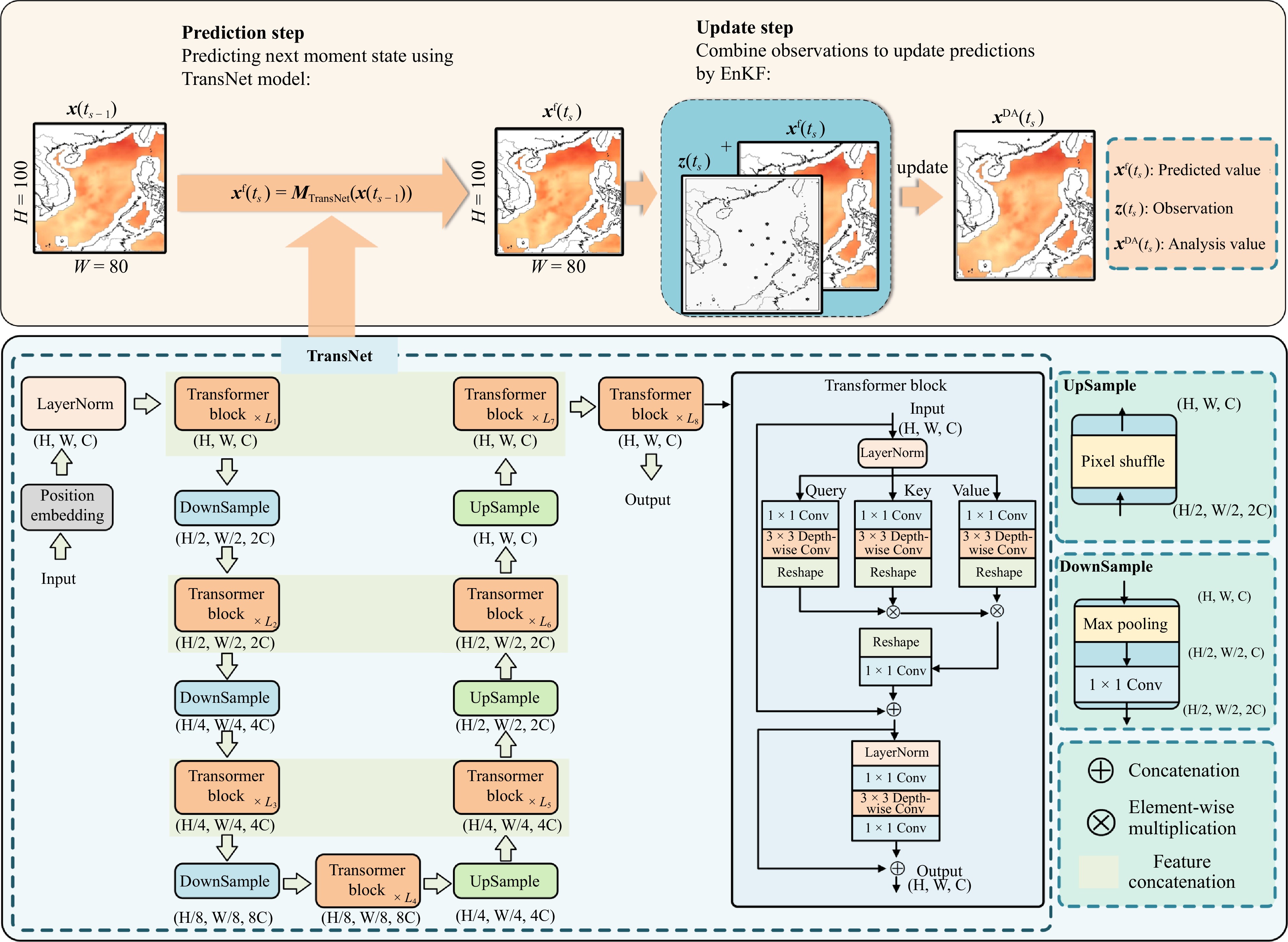
Since the attentional mechanism itself cannot discern the order of the sequence, we first encode the explicit positional information of these signal fragments to enhance their sequential information. In our model, we generate unique encodings for each position in the sequence based on sine and cosine functions at different frequencies. The position encoding is created using the following equations:

In these formulas, $ \mathrm{p}\mathrm{o}\mathrm{s} $ represents the position of the token in the sequence, $ i $ denotes the dimension, and $ {d}_{\mathrm{m}\mathrm{o}\mathrm{d}\mathrm{e}\mathrm{l}} $​ is the dimensionality of the model. These position encodings are added to the input embeddings to ensure that positional information is incorporated into the model.

For the ocean surface latent heat flux data input $ \in {\mathbb{R}}^{H\times W\times T} $ recorded every 3 hours, where $ H\times W $ represents the spatial dimensions and $ T $ denotes time, a $ 3\times 3 $ convolution is initially used for potential feature representation $ {\mathit{I}}_{0}\in {\mathbb{R}}^{H\times W\times C} $. Features $ {\mathit{I}}_{0} $ first enter the Layer Normalization (LayerNorm) module, which normalizes the input data for each feature. LayerNorm is a technique used to stabilize and accelerate the training process of deep neural networks. By normalizing the inputs, it reduces internal covariate shift, which refers to the changes in the distribution of network activations due to the updates of the parameters. This stabilization allows the model to converge faster and perform better. Specifically, LayerNorm computes the mean and variance of the input features and scales them to have zero mean and unit variance. This normalization helps in maintaining the distribution of the inputs consistent across different layers and training iterations.

As shown in Table 1, the input features $ {\mathit{I}}_{0} $ are processed through a four-stage encoder. In the first stage, two consecutive Transformer blocks are employed. This is followed by the second stage, which uses three Transformer blocks. The third stage processes the output through four Transformer blocks, and the final stage utilizes four Transformer blocks. Each stage incrementally refines the features, building upon the previous stage (Le Gallo et al., 2023). After each encoder stage, the size of the feature map is halved and the channel count is doubled. Eventually, the encoder generates four scaled feature maps with initial input feature sizes of 1, 1/2, 1/4, and 1/8, corresponding to 32, 64, 128, and 256 channel numbers, respectively. This process includes downsampling, implemented using max pooling (Stergiou and Poppe, 2023). Max pooling reduces the spatial dimensions of the feature maps while retaining the most important features by taking the maximum value within each pooling window. This progressive reduction in spatial dimensions combined with the increase in channel count allows the model to focus on the most salient features of the input data, enhancing its ability to learn complex representations. The decoder has the same structure as the encoder, doubling the feature size and halving the number of channels after each stage (Shan et al., 2018). The layered features from the encoder help to recover high-quality data step by step. A pixel shuffling operation is utilized while upsampling the features. Then, a $ 3\times 3 $ convolution block is applied to the highly seminal feature representation $ {\mathit{O}}_{0} $ to predict the ocean surface latent heat flux data. Real-time observations were incorporated into the model predictions using EnKF so that real-time corrections could be made to ensure accuracy and utility (Rafieeinasab et al., 2014).

Table  1.  Training setting of the model

Module	Setting	Size
Datasets	Input dimension	(100, 80, 1)
	Output dimension	(100, 80, 1)
	Training/Validation/Test Split	2000~2019/ 2020/2021
Encoder	Number of Layer	4
	Number of Transformer Blocks	[2,3,4,4]
	Embedding Dimensions	[32,64,128,256]
	Norm layer	LayerNorm
Decoder	Number of Layer	4
	Number of Transformer Blocks	[2,3,4,4]
	Embedding Dimensions	[32,64,128,256]

 | Show Table

DownLoad: CSV

3.1 Transformer encoder and decoder architecture

The Transformer model has been widely used since it was proposed, initially for natural language processing tasks such as machine translation (Jurisic et al., 2018). Its architecture is based on the attention mechanism, which differs from traditional recurrent neural networks and convolutional neural networks (Usama et al., 2020). The Transformer model has achieved success due to its efficient parallel computing capability, powerful representation learning, and adaptability to long-distance dependencies. It has been widely applied to various NLP tasks such as text generation, text classification, and question answering systems, and has also gained great success in the field of pre-trained language models. In this study, we combined convolution operations with Transformer blocks to process two-dimensional data. By incorporating convolutional operations into the multi-head self-attention mechanism of the transformer block, we have designed a transformer block for predicting latent heat fluxes at the ocean surface. The encoder and decoder of the model consist of multiple Transformer block layers.

When designing the Transformer block, we introduced convolution operations to achieve spatial information interaction. Specifically, we chose to compute attention along the channel dimension instead of the traditional spatial dimension, ensuring consistency in calculations across any spatial range. This approach better captures and processes the complex spatial information within large sea areas, thereby completing ocean prediction tasks more accurately (Niu et al., 2021).

As shown in the TransNet structure in Fig. 2, for the input features $ \mathit{I}\in {\mathbb{R}}^{H\times W\times C} $, we start by applying layer normalization to generate the query $ \mathit{Q}\in {\mathbb{R}}^{H\times W\times C} $, the key $ \mathit{K}\in {\mathbb{R}}^{H\times W\times C} $, and the value $ \mathit{V}\in {\mathbb{R}}^{H\times W\times C} $. Following this, a $ 1\times 1 $ convolutional layer captures the channel features, and $ 3\times 3 $ depthwise separable convolution processes the spatial features. The reshape operation then converts $ \text{Q} $, $ \mathit{K} $, and $ \mathit{V} $ into token sequences, resulting in $ {\mathit{Q}}^{\mathit{\text{'}}}\in {\mathbb{R}}^{{C}^{\text{'}}\times H\times W} $, $ {\mathit{K}}^{\text{'}}\in {\mathbb{R}}^{H\times W\times {C}^{\text{'}}} $, and $ {\mathit{V}}^{\text{'}}\in {\mathbb{R}}^{{C}^{\text{'}}\times H\times W} $. The matrices $ {\mathit{Q}}^{\text{'}} $ and $ {\mathit{K}}^{\mathit{\text{'}}} $ are multiplied, and the softmax operation is applied to generate the attention map $ \mathit{M}\in {\mathbb{R}}^{{C}^{\text{'}}\times {C}^{\text{'}}} $. The value $ {\mathit{V}}^{\mathit{\text{'}}} $ is multiplied by the attention map matrix to produce the output $ {\mathit{O}}^{\mathit{\text{'}}}\in {\mathbb{R}}^{{C}^{\text{'}}\times H\times W} $. Finally, a $ 1\times 1 $ convolution adjusts the number of output channels, and a residual connection with the input is performed to obtain the final output $ \mathit{O}\in {\mathbb{R}}^{C\times H\times W} $. The generation of $ \mathit{Q} $, $ \mathit{K} $, and $ \mathit{V} $ is a key step in the self-attention mechanism, and these vectors help the model understand and emphasize key information in the input data by calculating the attention weights. Although the self-attention mechanism can effectively handle long-range dependencies, it does not directly optimize for spatial or local features of the input data in its original form. By adding a convolutional layer after the generation of $ \mathit{Q} $, $ \mathit{K} $, and $ \mathit{V} $, we can enhance the capability of the model to capture spatial features of the input data without changing the parameter dimensions, facilitating spatial information interaction.

Since the Transformer module does not compute attention along the spatial dimension, its ability to capture spatial features is weakened. Therefore, convolution operations are needed in the feed-forward network to further enhance spatial information interaction. We use a $ 1\times 1 $ convolution to replace fully connected operations and insert a $ 3\times 3 $ depthwise separable convolution between two $ 1\times 1 $ convolutions to enhance the spatial information extraction capability of the model.

3.2 Ensemble Kalman Filter

DA optimizes model state estimation by integrating observations and model predictions. It is a crucial technology in many geoscience fields, and plays an essential role in weather forecasting and ocean sciences in particular (Reichle, 2008). DA improves the accuracy and reliability of model predictions by using real-time or historical observations to further improve model predictions, thus ensuring that model outputs are closer to true values (Bouttier and Courtier, 2002).

EnKF as a DA technique is widely used due to its unique advantages (Cheng et al., 2023). In the context of our study, EnKF is integrated into the TransNetDA framework to ensure the accuracy and reliability of ocean surface latent heat flux predictions. EnKF applies Monte Carlo techniques to Bayesian update problems (Tierney and Mira, 1999), using a set of stochastic realizations to approximate the state of dynamic systems effectively. The state matrix of the ensemble comprises all individual state vectors:

where $ {\mathcal{X}}_{k}\left(t\right) $ denote the $ k $th member of ensembles at time $ t $, $ {N}_{x} $ the dimension of each vector, and $ {N}_{e} $ the size of ensembles.

EnKF operates through two major phases: prediction and updating (Cheng et al., 2023). During prediction, the prediction of each ensemble member is independently calculated using the following model:

where $ {\mathcal{M}}_{\mathrm{T}\mathrm{r}\mathrm{a}\mathrm{n}\mathrm{s}\mathrm{N}\mathrm{e}\mathrm{t}} $ denotes the TransNet (without DA) prediction model, $ {\mathcal{X}}_{k}\left({t}_{s-1}\right) $ is the kth member of the ensemble of predicted values from the previous moment, and the mean of the ensemble is the final predicted value at $ {t}_{s-1} $.

The average of all forecasts provides the ensemble mean at time $ {t}_{s} $:

Covariance of the prediction error, $ {\mathit{P}}^{\mathrm{f}} $, is computed as:

$ \mathcal{Z}\left({t}_{s}\right) $ represents the noisy ocean surface latent heat flux data observed at $ {t}_{s} $, ranging over the entire study area, with ocean latent heat flux data values at each grid point plus random noise drawn from $ N\left(0,{\sigma }_{\text{obs}}\right) $, where $ {\sigma }_{\text{obs}} $ is the standard deviation of the data on all grid points from 2000 to 2019. Although adding Gaussian random noise to the true data is an approximation, it is a common practice in the data analysis literature (Brajard et al., 2020; Lindgren et al., 2022). This approach allows accurate evaluation of the performance of the algorithm without interference from external variables (Li et al., 2024). Upon receiving new observations $ \mathcal{Z}\left({\mathrm{t}}_{\mathrm{s}}\right) $ at $ {t}_{s} $, the update phase adjusts each ensemble member, the obtained $ {\mathcal{X}}_{k}^{\mathrm{D}\mathrm{A}}\left({t}_{s}\right) $ is the $ k $th member of ensembles prediction of the TransNetDA model at $ {t}_{s} $:

the Kalman gain $ \mathit{K}\left({t}_{s}\right) $ is formulated as:

and the analysis ensemble is averaged to produce the final analysis values, which is the final predicted value at time $ {t}_{s} $:

where $ \mathcal{R}={{\sigma }}^{\mathrm{obs}}\mathit{I} $ specifies the observation error covariance, ensuring the relevance of updates, and $ {{\sigma }}^{\mathrm{o}\mathrm{b}\mathrm{s}} $ is the standard deviation of the observations. Finally, the post-update covariance matrix $ {\mathit{P}}^{\mathrm{D}\mathrm{A}}\left({t}_{s}\right) $ is calculated as:

In our implementation, the real-time observations of ocean surface latent heat flux are continuously fed into the model. EnKF adjusts the model states by minimizing the difference between the predicted and observed values, thus correcting the predictions in real time. This process not only enhances the predictive accuracy of the model but also improves its robustness against uncertainties in the data.

By combining the strengths of the Transformer architecture for feature extraction and EnKF for real-time DA, TransNetDA provides a powerful tool for precise and efficient ocean surface latent heat flux prediction. The prediction of the TransNetDA model includes two phases, which are the initial prediction of TransNet and the prediction after assimilation using observations, where the assimilation step involves the DA between the predictions of the TransNet model and the real-time observations. The TransNet model is responsible for providing the initial predictions based on the historical data, which serve as the background values to be used in the DA phase, and subsequently by integrating the observations to further obtain analysis values, whose values are used as predictions for DA, which are the final predictions of the TransNetDA model. For the convenience of presenting the results, the predicted values of TransNetDA shown below refer to the final predicted values after performing the ensemble averaging process.

4. Results

4.1 Performance criteria

Two key metrics are used in this study to assess model performance: root mean square error (RMSE) and coefficient of determination ($ {\mathrm{R}}^{2} $) (Chicco et al., 2021). Before performing the evaluation, outliers were removed and missing values were processed using bilinear interpolation to prevent them from affecting the results. First, the RMSE is a widely used measure of the differences between predicted and observed values. It quantifies the average magnitude of the prediction errors, giving a clear indication of the predictive accuracy of the model, the RMSE is calculated as follows:

where $ m $ represents the sample size of all data points in the studied sea area, $ y $ is the true value, and $ \widehat{y} $ is the predicted value. Lower RMSE indicates that the prediction accuracy of the model is higher. The RMSE comparison is based on the sum of the squared differences of the processed data points. $ {\mathrm{R}}^{2} $ is used to measure the proportion of variance in the observed data that can be predicted by the model. It is a statistical measure that indicates how well the data match the statistical model and is defined as follows:

where $ \bar{y} $ is the mean value of $ y $. The closer the value of $ {\mathrm{R}}^{2} $ is to 1, the more adequately the model explains the variability of the data. Similar to RMSE, the $ {\mathrm{R}}^{2} $ comparison is also based on the total difference between the processed data points.

Combining RMSE and $ {\mathrm{R}}^{2} $ allows a comprehensive assessment of the predictive accuracy of the model and its explanatory power, thus effectively comparing the performance of different models. RMSE provides insight into the average magnitude of the errors, while $ {\mathrm{R}}^{2} $ indicates how well the variability of the data are captured by the model. By employing both metrics, this study effectively compares the performance of different models, ensuring a robust evaluation of their predictive capabilities.

4.2 Model comparison

Changes in ocean surface latent heat flux influence ocean surface temperatures, thereby affecting global ocean circulation and climate patterns (Large and Yeager, 2012). Therefore, developing efficient prediction tools holds significant scientific value and potential for meteorological and oceanographic research applications. The Transformer has powerful feature extraction capabilities, allowing it to extract high-level and complex features from multidimensional data, and it excels in predicting ocean surface latent heat flux. EnKF can enhance the performance of the Transformer model in ocean data prediction. By assimilating observations into model predictions and continuously updating the model states, the predictions of the Transformer become closer to actual observations. Specifically, we perform DA every 6 hours using random noise generated from a normal distribution $ N\left(0,{\sigma }_{\text{obs}}\right) $ to correct the prediction trajectories. We perform iterative multi-step predictions using the well-trained TransNetDA model and apply EnKF to assimilate observations at the end of each DA cycle (Gharamti et al., 2017).

In this section, we compare the performance of TransNetDA with ConvLSTM, LSTM, and U-Net to predict hourly ocean surface latent heat flux and compare it with accurate data. The performance of these models is evaluated by predicting the periods of ocean surface latent heat flux. These models predict the change in ocean surface latent heat flux values over the next 24 hours by learning from historical data, starting at 01:30 and getting a prediction every 3 hours. Additionally, we compare with two baseline models such as persistence (Kessler et al., 2016) and climatology (historical day-of-year mean and variance) models (Ward et al., 2014). The persistence approach, which predicts future values based on current or past values, can be used to predict the dynamics of high inertia systems, which are common in lakes and reservoirs. The Climatology model, based on historical observations, uses long-term averages at the same time of year to predict future conditions. This method performs better in long-term predictions, especially when the dynamics are dominated by repetitive seasonal cycles (Olsson et al., 2024). The performance of these models is evaluated using RMSE and $ {\mathrm{R}}^{2} $ as metrics, comparing the predicted results with actual data.

As shown in Table 2, TransNetDA performs excellently predicting ocean surface latent heat flux. At 01:30, the RMSE of TransNetDA is 2.385, increasing to 7.227 at 04:30 and decreasing to 4.785 at 07:30. Additionally, the $ {\mathrm{R}}^{2} $ of TransNetDA is highest at 01:30 at 0.997, followed by 0.985 at 07:30 and 0.970 at 04:30. These results indicate that TransNetDA maintains high prediction accuracy over time due to EnKF corrections.

Table  2.  The $ {\mathrm{R}}^{2} $ and RMSE values of four models on January 1, 2021 at 01:30, 04:30, and 07:30, respectively.

Model	01:30			04:30			07:30
	$ {\mathrm{R}}^{2} $	RMSE		$ {\mathrm{R}}^{2} $	RMSE		$ {\mathrm{R}}^{2} $	RMSE
Persistence	0.899	18.716		0.956	9.993		0.962	8.739
Climatology	0.471	42.851		0.406	41.935		0.339	43.109
U-Net	0.973	6.945		0.907	11.875		0.859	14.215
LSTM	0.929	10.354		0.863	13.801		0.786	17.633
ConvLSTM	0.955	8.283		0.894	12.315		0.835	15.504
TransNetDA	0.997	2.385		0.970	7.227		0.985	4.785

 | Show Table

DownLoad: CSV

In contrast, the RMSE of U-Net is 6.945 at 01:30, 11.875 at 04:30, and 14.215 at 07:30. The $ {\mathrm{R}}^{2} $ of U-Net is 0.973 at 01:30, dropping to 0.907 at 04:30 and 0.859 at 07:30, indicating a decreased prediction accuracy over time. The RMSE of ConvLSTM is 8.283 at 01:30, 12.315 at 04:30, and 15.504 at 07:30. The $ {\mathrm{R}}^{2} $ of ConvLSTM reaches its highest value of 0.955 at 01:30, followed by 0.894 at 04:30 and 0.835 at 07:30. These results show that the prediction accuracy of ConvLSTM decreases faster compared to TransNetDA. The RMSE of LSTM is 10.354 at 01:30, 13.801 at 04:30, and 17.633 at 07:30. The $ {\mathrm{R}}^{2} $ of LSTM is 0.929 at 01:30, 0.863 at 04:30, and 0.786 at 07:30, indicating the lowest prediction accuracy among the evaluated models.

For Persistence, the RMSE is 18.716 at 01:30, decreasing to 9.993 at 04:30, and further to 8.739 at 07:30. The $ {\mathrm{R}}^{2} $ of Persistence is 0.899 at 01:30, increasing to 0.956 at 04:30, and slightly improving to 0.962 at 07:30. These results suggest that while Persistence shows a reduction in error over time, its overall performance is less accurate compared to TransNetDA. Climatology exhibits the highest RMSE values among all models, with 42.851 at 01:30, 41.935 at 04:30, and 43.109 at 07:30. The $ {\mathrm{R}}^{2} $ of Climatology is 0.471 at 01:30, 0.406 at 04:30, and 0.339 at 07:30, demonstrating that Climatology is the least accurate method for predicting ocean surface latent heat flux.

The comparison of RMSE and $ {\mathrm{R}}^{2} $ clearly shows that TransNetDA outperforms other models in predicting ocean surface latent heat flux. TransNetDA provides more accurate predictions and stronger interpretability than traditional artificial neural network methods (Salahuddin et al., 2022).

TransNetDA, due to its multi-scale attention mechanism, enables the model to focus on critical regions at different scales. This mechanism enhances the ability of the model to capture complex spatial patterns and ocean surface latent heat flux dynamics, resulting in more accurate predictions. In contrast, although U-Net has strong feature extraction capabilities, it needs the design to specifically emphasize multi-scale features, limiting its performance in handling complex meteorological data. Although ConvLSTM and LSTM perform well in processing time series data, they need help to capture and integrate multi-scale spatial features. ConvLSTM improves upon LSTM by incorporating spatial information, but both models face challenges when handling very long data sequences, potentially encountering gradient-related issues that affect prediction accuracy. Persistence, while simple and often effective for short-term predictions, shows significant limitations as it relies solely on the latest observations, leading to larger errors over longer periods (Gong and Wang, 1998). Climatology can predict future climate states by averaging historical data (Liu et al., 2023), but its reliance on long-term averages does not capture short-term changes or anomalies in climate. EnKF continuously corrects model predictions, reducing cumulative errors in long-term forecasts and ensuring the stability and accuracy of the Transformer model in long-term predictions. During the model training process, EnKF can integrate real-time observations, which improves the learning ability and prediction performance of the model (Chen et al., 2011).

4.3 Evaluation of TransNetDA predictions

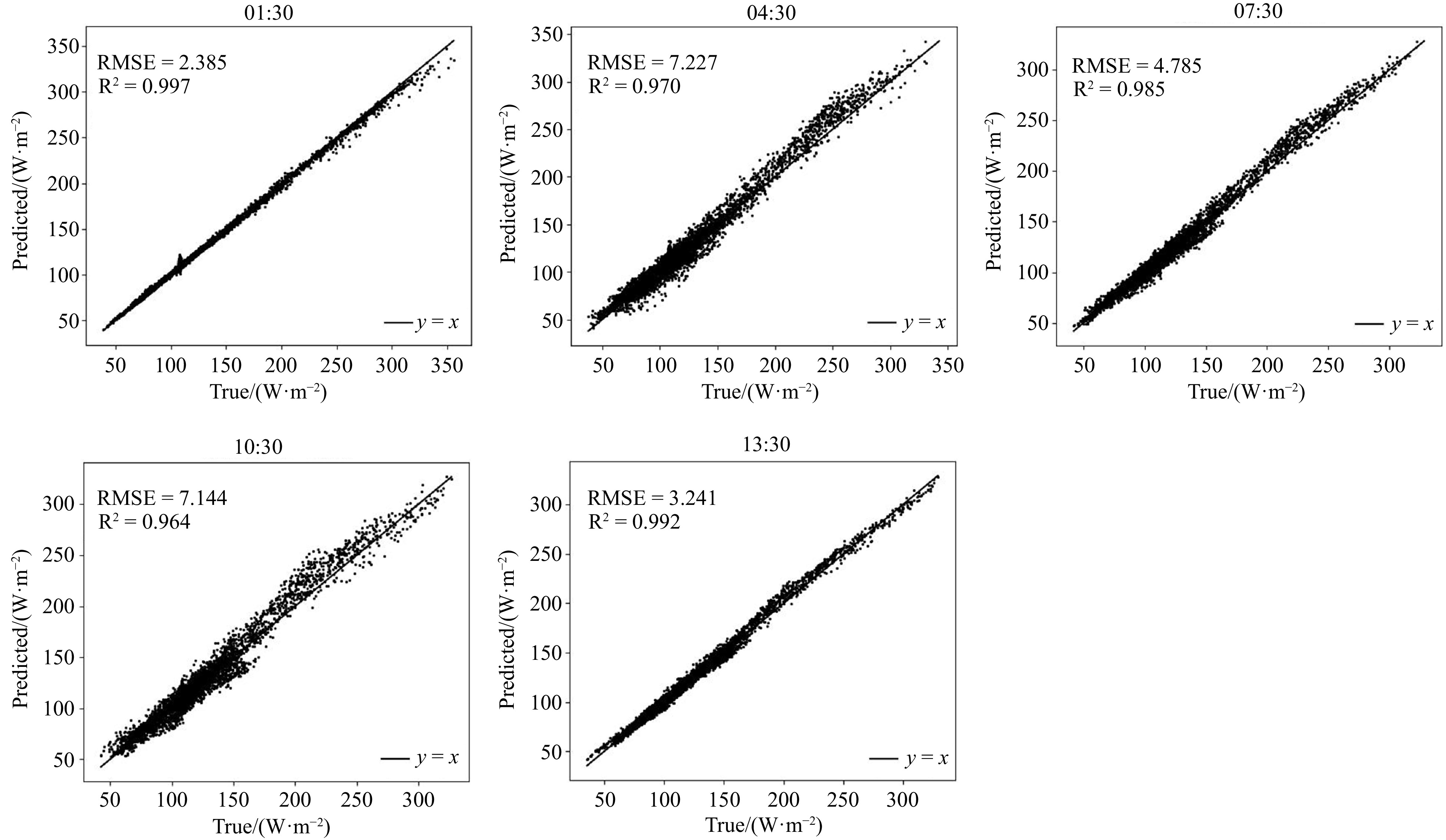
In this section, to further demonstrate the predictive performance of the TransNetDA model, we compare the predicted and true values of ocean surface latent heat fluxes at different times in different months. We use scatterplots to evaluate these comparisons. In particular, we present results for all days at different time points in January, March, May, and July, where the number of points per subplot for each month is 248 000 (8 000 points per day per hour).

Figure 3 shows the predicted values of the TransNetDA model against the true values at multiple time points in January. The $ {\mathrm{R}}^{2} $ values range from 0.975 to 0.994, indicating a high correlation between the predicted and true values. The RMSE values range from 3.153 to 6.258, demonstrating the predictive accuracy of the model. The scatter region around the $ y=x $ line indicates that the model performs well in predicting the ocean surface latent heat flux for the month. This phenomenon indicates that the model was well-calibrated in January, providing reliable estimates at different times of the day. Figure 4 demonstrates the performance of the model at the same time points in March, with $ {\mathrm{R}}^{2} $ values ranging from 0.970 to 0.991 and RMSE values ranging from 2.934 to 5.184. These results show consistent predictive performance compared to January, though with slightly higher RMSE values. The dense number of points around the $ y=x $ line continues to demonstrate the robustness of the model in predicting latent heat fluxes, maintaining high accuracy despite seasonal variations. This performance suggests that the model effectively generalizes to maintain its reliability under different seasonal conditions.

Figure  3.  Scatterplot of TransNetDA model predictions vs. true data in January.

DownLoad: Full-Size Img PowerPoint

Figure  4.  Scatterplot of TransNetDA model predictions vs. true data in March.

DownLoad: Full-Size Img PowerPoint

The scatterplots for May show a range of $ {\mathrm{R}}^{2} $ values from 0.961 to 0.990 and RMSE values from 2.284 to 4.403 (Fig. 5). These results indicate an improvement in prediction accuracy compared to previous months, with lower RMSE values signifying better model performance. The scatter distribution remains concentrated around the $ y=x $ line, confirming the accuracy of the model. In July, the scatterplots show $ {\mathrm{R}}^{2} $ values ranging from 0.972 to 0.992 and RMSE values ranging from 2.179 to 4.218 (Fig. 6). This performance is consistent with that of May, demonstrating high predictive accuracy and a slight improvement in RMSE values. These plots show that the model maintains its predictive ability across different months and times. The stability of model performance during the peak summer months, when latent heat fluxes are typically high, demonstrates its robustness and versatility in dealing with extreme conditions.

Figure  5.  Scatterplot of TransNetDA model predictions vs. true data in May.

DownLoad: Full-Size Img PowerPoint

Figure  6.  Scatterplot of TransNetDA model predictions vs. true data in July.

DownLoad: Full-Size Img PowerPoint

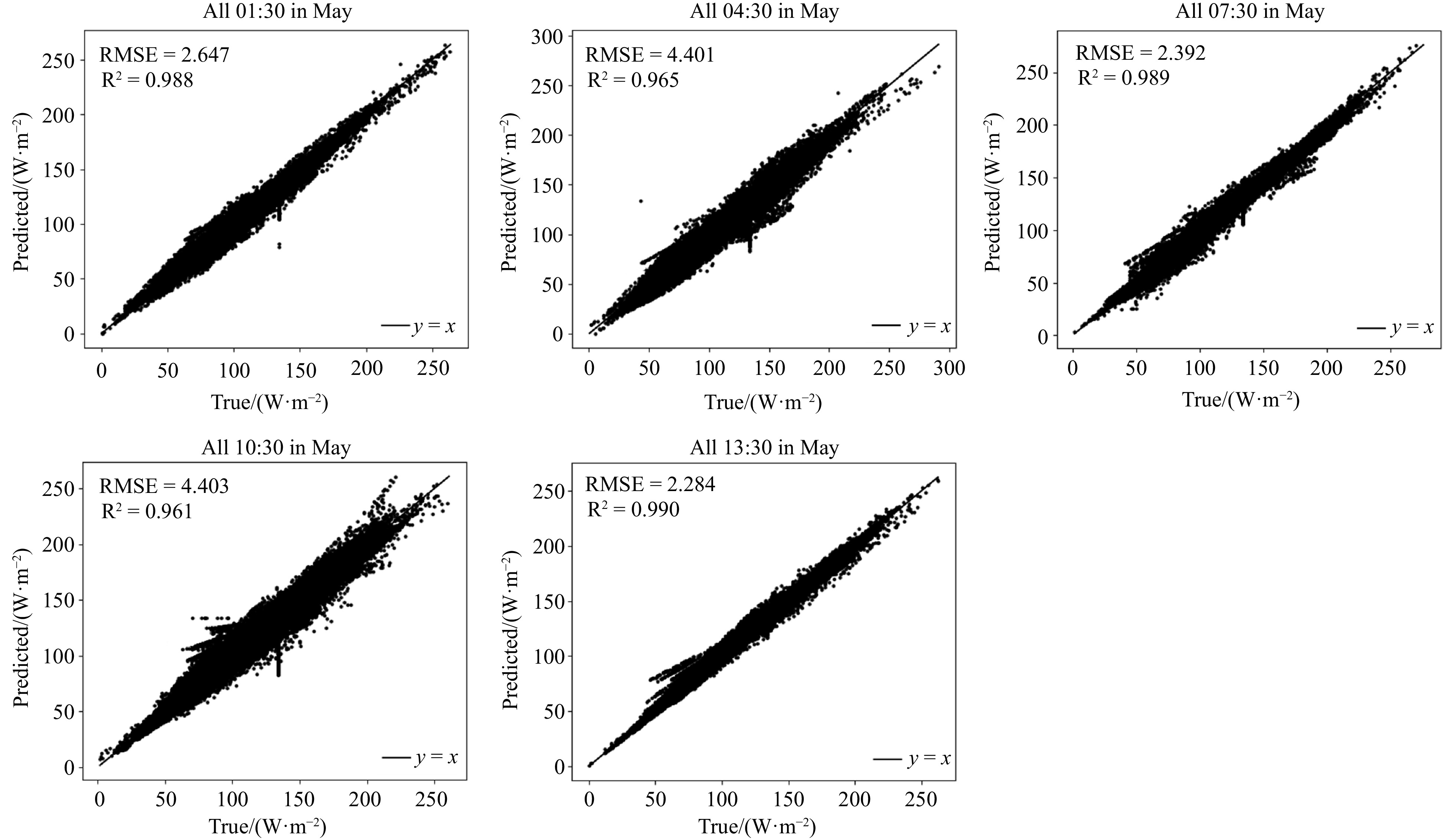
The significant improvement in prediction accuracy at 07:30 and 13:30 compared to the previous times (01:30, 04:30, and 10:30) can be attributed to the integration of DA techniques. DA enhances model predictions by incorporating observations and improving the initial conditions. At 07:30 and 13:30, the increased availability and incorporation of observed data allowed the TransNetDA model to more effectively correct discrepancies between model predictions and observed data. This resulted in higher $ {\mathrm{R}}^{2} $ values and lower RMSE values, indicating a closer approximation to the true values and improved overall model performance. The significant improvement highlights the crucial role of DA in enhancing prediction accuracy. These results validate the effectiveness of the TransNetDA model in providing accurate and reliable forecasts across different months and times, emphasizing its potential for wider application in oceanographic research.

4.4 Model validation

In this section, we present the validation results of the TransNet model. In our model training process, 58 424 samples are used for training and 2 928 samples are used for validation. The labels used to train the TransNet model are the ocean surface latent heat flux data values per three hours in the ocean surface latent heat flux dataset. The network structure parameters of the TransNet model are listed in Table 1. The training and prediction are performed on a server with an NVIDIA Tesla A100 GPU, 128 GB of RAM, and 2 TB of storage. The operating system used is Ubuntu 20.04, with the main tools and libraries including Python 3.8 and TensorFlow 2.4.

The training and validation loss and accuracy curves for the TransNet model are shown in Fig. 7. The subplot on the left displays the loss curves, where both the training and validation losses continue to decrease as the number of training rounds increases. Around round 100, the validation loss shows a significant decrease and aligns closely with the training loss, indicating that the model generalizes well and is not overfitting. By round 200, both curves begin to level off, suggesting that the model has reached a steady state. The final training and validation loss values are close and fluctuate less, confirming the robustness of the model.

Figure  7.  Loss and accuracy curves for model training and validation.

DownLoad: Full-Size Img PowerPoint

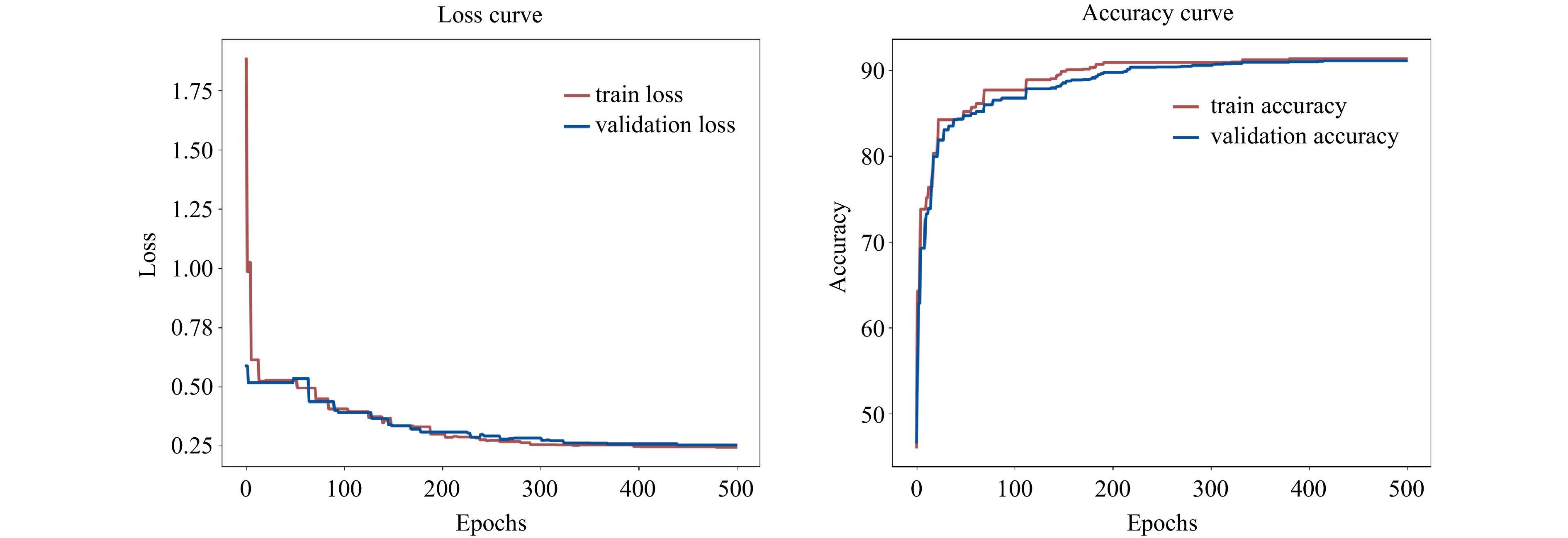
The right subplot shows the accuracy curves for training and validation. As the number of training rounds increases, the model reaches about 80% accuracy by round 50, and the rate of improvement begins to slow down. This indicates that the model is effectively capturing the underlying patterns of the data. Between rounds 50 and 100, the accuracy continues to steadily improve, reaching approximately 90%. After this point, the accuracy curve begins to flatten, suggesting that the model is approaching its maximum performance. From round 200 onwards, the training and validation accuracy curves converge and stabilize at approximately 92%. The tight alignment of these curves throughout the training process indicates that the performance of the model on the training and validation datasets remains consistent without significant overfitting.

In summary, the training process visualized by the loss and accuracy curves shows that the TransNet model maintains good generalization performance on the validation data while learning effectively from the training data. The convergence of the loss and accuracy curves indicates that the model achieves a high level of performance while minimizing the risk of overfitting.

4.5 Ablation experiments

We conduct ablation experiments in order to assess the impact of DA using EnKF in the TransNet model. The experiment aims to understand the importance of DA and its contribution to improving the performance of ocean surface latent heat flux prediction. By comparing and analyzing the performance of TransNetDA (Fig. 8) and TransNet (Fig. 10), we found that there is a significant difference in prediction accuracy between the two models. Compared to the standard TransNet model, TransNetDA, which incorporates EnKF for DA, outperforms the standard TransNet model in terms of metrics and frequency of DA. The results show that TransNetDA has lower RMSE values and higher $ {\mathrm{R}}^{2} $ values at all time points. As shown in Fig. 9 (each subplot has 8 000 points), the RMSE of TransNetDA is 2.385 and $ {\mathrm{R}}^{2} $ is 0.997, then at 04:30 without DA the RMSE increases and $ {\mathrm{R}}^{2} $ decreases, at 07:30 after using TransNetDA the RMSE decreases and $ {\mathrm{R}}^{2} $ increases again, and at 10:30 and 13:30 similar trends, indicating a significant improvement in model prediction ability after using DA.

Figure  8.  Comparison of 01:30, 07:30 and 13:30 real data (left), hourly TransNetDA prediction (center), and the differences between them (right) on January 1, 2021. DA frequency is opted as 6 hours for this experiment.

DownLoad: Full-Size Img PowerPoint

Figure  9.  Scatterplot of TransNetDA model predictions vs. true data on January 1, 2021.

DownLoad: Full-Size Img PowerPoint

Figure  10.  Comparison of 01:30, 07:30 and 13:30 real data (left), hourly TransNet prediction (center), and the differences between them (right) on January 1, 2021.

DownLoad: Full-Size Img PowerPoint

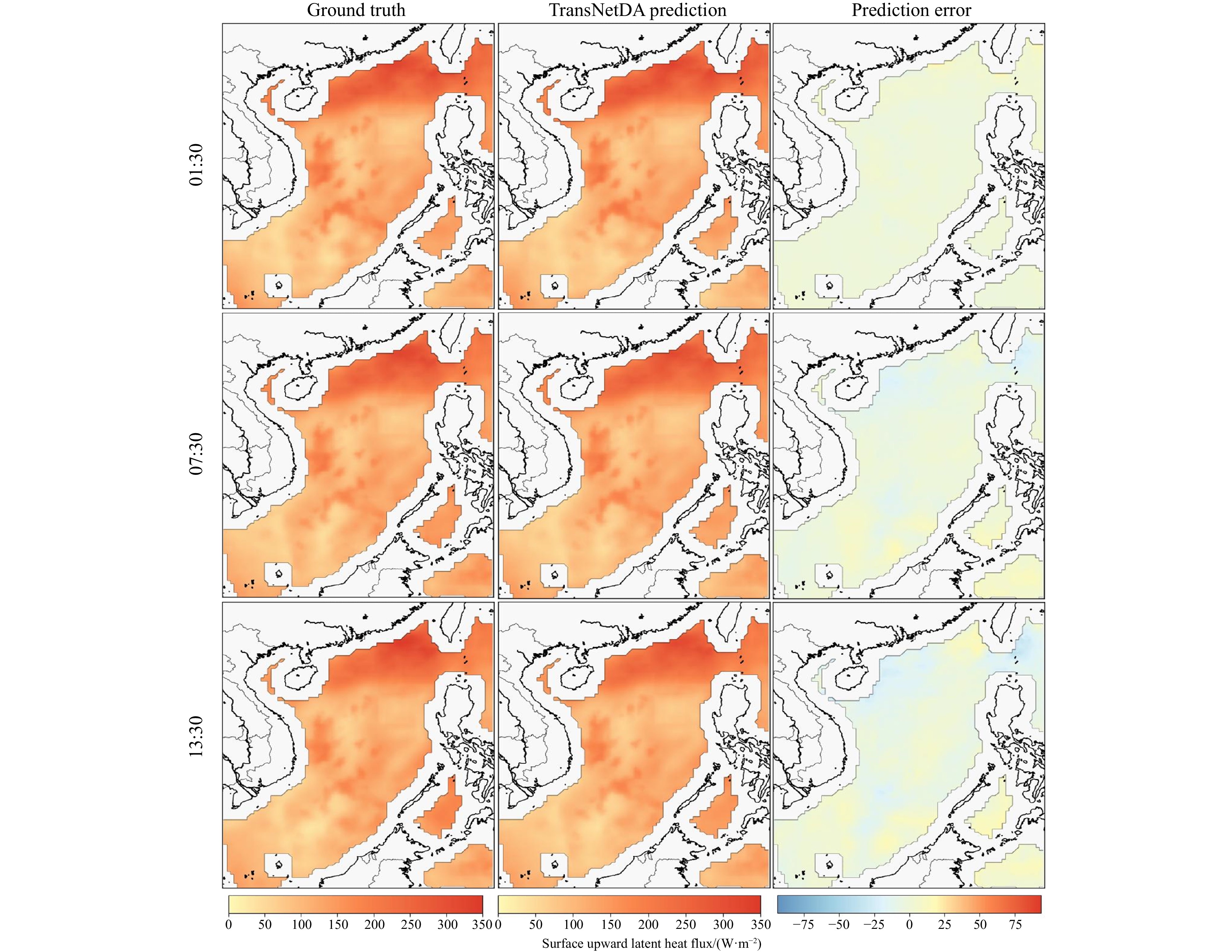
In summary, the integration of EnKF into the TransNet framework to form TransNetDA demonstrates the key role of DA in improving model performance. Higher accuracy and stability achieved through EnKF. Ablation experiments confirmed frequent DA is essential to maintain high prediction accuracy and effectively manage uncertainty in marine data. Throughout the study period, the RMSE of the method remained below 10 W/m², and the $ {\mathrm{R}}^{2} $ value was above 0.90. These performance metrics indicate that TransNetDA can effectively capture the spatial distribution of ocean surface latent heat flux data.

4.6 Impact of DA frequency on prediction performance

To systematically analyze the impact of DA frequency on operational prediction performance, this study explores the effects of different assimilation frequencies to determine the optimal frequency for use in actual observations (Durand and Margulis, 2006). Specifically, we evaluated three DA frequencies: every 6 hours, 12 hours, and 24 hours (Fig. 11).

Figure  11.  Evaluate the prediction accuracy of the TransNetDA on January 1, 2021 at different DA frequencies (6, 12 and 24 hours).

DownLoad: Full-Size Img PowerPoint

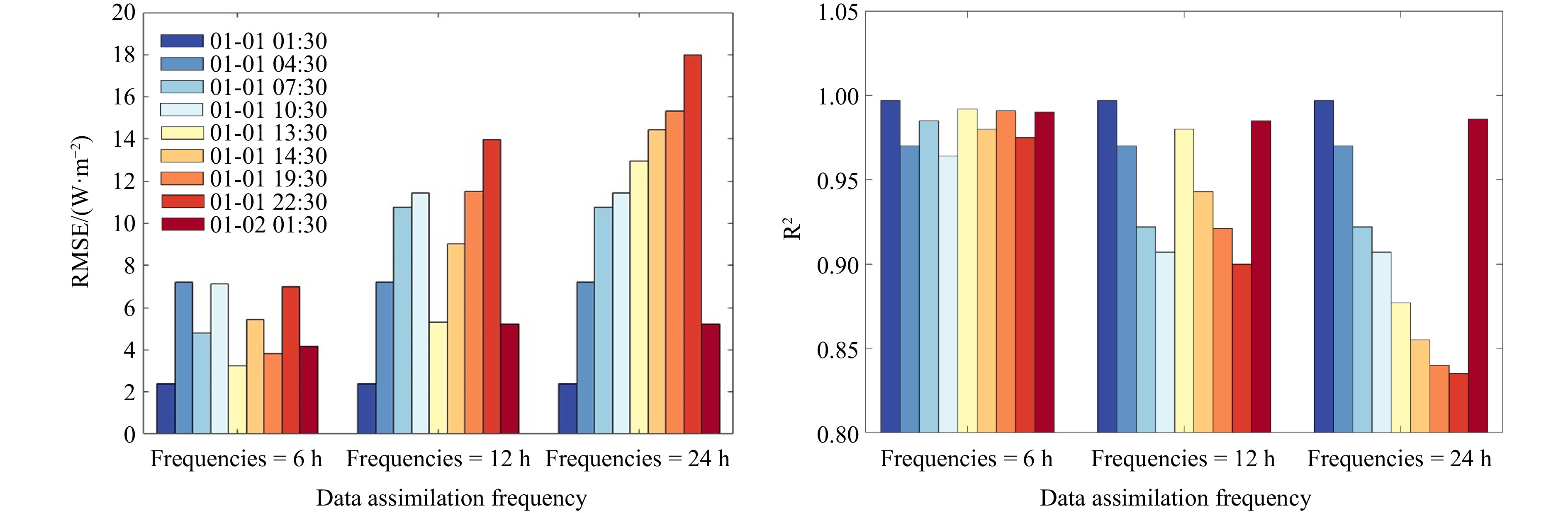
By selecting these frequencies, we systematically assessed the specific impact of different DA strategies on prediction accuracy (Geer et al., 2018). The evaluation focused on calculating the RMSE and $ {\mathrm{R}}^{2} $ to compare the predicted values with baseline data. Our research results show that within each DA cycle, RMSE gradually increases (Oke et al., 2008), while $ {\mathrm{R}}^{2} $ correspondingly decreases. This pattern underscores the enhanced prediction accuracy achieved by incorporating observations at the end of the cycle. Notably, at the end of each DA cycle, we observed significant variations in RMSE and $ {\mathrm{R}}^{2} $ due to changing meteorological conditions (Pan et al., 2008). These refined predictions are then used as the initial conditions for the following DA cycle, continuously improving the predictive accuracy of the model.

The results indicate that shortening the DA cycle can improve prediction accuracy (Ruiz et al., 2013). The critical role of DA frequency in enhancing the prediction performance of ocean surface latent heat flux has been confirmed. Frequent DA can reduce prediction errors, enhance the correlation between the model and actual meteorological data, and improve the reliability and utility of the predictions (Liu et al., 2012; Yucel et al., 2015). The TransNetDA method performs excellently in predicting ocean surface latent heat flux, especially when the DA frequency is set to every 6 (Fig. 8) and 12 hours. As shown in Fig. 11, these data regions further validate the high performance of the combination of TransNet and EnKF in DA, significantly enhancing the accuracy and stability of ocean surface latent heat flux prediction.

DA is crucial for improving the accuracy and reliability of model predictions. By incorporating real-time observations, EnKF helps correct prediction trajectories, reduce errors, and enhance the correlation between model predictions and actual observations (Liu et al., 2016). This continuous correction ensures that the model remains consistent with the ever-changing ocean environment. The results of the ablation experiments show that frequent DA (every 6 hours) resulted in the highest prediction accuracy, with TransNetDA maintaining low RMSE values and high $ {\mathrm{R}}^{2} $ values throughout the study period. In addition, this study systematically explores the effect of DA frequency. Frequent DA reduces the prediction error and enhances the ability of the model to capture and integrate the spatial and temporal complexity of ocean surface latent heat fluxes.

5. Discussion

This study presents TransNetDA, which combines the Transformer architecture and the EnKF to accurately predict ocean surface latent heat fluxes. By comparing with a variety of baseline models, including Persistence, Climatology, U-Net, LSTM and ConvLSTM, the TransNetDA model is highly effective in terms of prediction accuracy and reliability. Firstly, the Transformer component in TransNetDA excels in feature extraction, capturing complex spatio-temporal dependencies in the data using its multi-head self-attention mechanism. Secondly, EnKF plays a key role in assimilating real-time observations and continuously updating model predictions to reduce errors and improve accuracy. This combination ensures that TransNetDA maintains high prediction accuracy over a long period.

The results of this study emphasize the effectiveness of frequent DA. By integrating observations every six hours, TransNetDA achieves optimal performance, characterized by the lowest RMSE values and the highest $ {\mathrm{R}}^{2} $ values. This finding highlights the importance of timely updating to maintain forecast accuracy and reliability under rapidly changing ocean conditions. Comparisons with conventional models show that TransNetDA performs well in capturing the spatial distribution and temporal dynamics of latent heat fluxes at the ocean surface. Furthermore, model performance evaluations at various time points on January 1, 2021 reveal that TransNetDA consistently maintains high accuracy over extended periods, reflecting its robustness and adaptability. These results suggest that frequent DA is essential for enhancing predictive capabilities and ensuring the reliability of oceanographic forecasts, thereby supporting better decision-making in maritime and climate-related applications.

Future research tasks involve combining TransNetDA with advanced deep learning methods, such as graph neural networks and generative adversarial networks, to enhance its ability to model complex non-linear relationships in the data. This integration aims to improve prediction accuracy and expand the applicability of the model in operational forecasting. It will also refine the accuracy and reliability of ocean surface latent heat flux predictions under sparse observations conditions, thereby providing timely and accurate forecasts for various oceanographic and environmental decision-making processes.

Conflict of interest

The authors declare no competing interests.