Xu Fang, Lujun Zhang. The evolution characteristics and causes of melt ponds in the Arctic Ocean[J]. Acta Oceanologica Sinica. doi: 10.1007/s13131-024-2390-z
Citation:
Xu Fang, Lujun Zhang. The evolution characteristics and causes of melt ponds in the Arctic Ocean[J]. Acta Oceanologica Sinica. doi: 10.1007/s13131-024-2390-z
Xu Fang, Lujun Zhang. The evolution characteristics and causes of melt ponds in the Arctic Ocean[J]. Acta Oceanologica Sinica. doi: 10.1007/s13131-024-2390-z
Citation:
Xu Fang, Lujun Zhang. The evolution characteristics and causes of melt ponds in the Arctic Ocean[J]. Acta Oceanologica Sinica. doi: 10.1007/s13131-024-2390-z
Melt ponds are significant physical features on the ice surface throughout the Arctic summer, and the scarcity of observational data has resulted in a vague understanding about it. This study employs satellite data and multi-model averaged outputs from CMIP6 to analyze the spatiotemporal evolution characteristics of Arctic melt ponds and their relationship with sea ice thickness (SIT) and atmospheric energy flux. The ponds first emerge at lower latitudes and gradually extend to cover central ice areas as the season progresses, then persisting longer and covering larger total areas in the central region, with peak areas exceeding 0.6 million km2, which is 4 to 5 times that of other marginal areas. Over the past two decades, pond coverage has exhibited markedly different trends with slight decreases in the marginal seas but significant increases in the central area. Both CMIP6 and satellite data indicate that the sea ice carrying capacity, related to thickness, plays a crucial role in creating these differences. There is a marked increasing pond in areas with thicker ice. When the SIT falls below a certain threshold, however, sea ice melting results in decreased pond coverage. Additionally, the energy balance on the ice surface also dramatically impacts pond changes. For instance, the overall pond changes in central area are influenced by net longwave radiation (NLR) and latent heat (LH), with anomalies in these fluxes correlating highly (up to 0.8) with pond anomalies. Meanwhile, net shortwave radiation (NSR) primarily causes local pond anomalies through the pond-shortwave feedback only under the clear weather conditions.
In recent years, polar changes characterized by decreasing sea ice and warming arctic have received widespread attention. Over the past 40 years, sea ice extent has sharply shrunk in all seasons, with a notable drop of more than 30% in summer (Kinnard et al., 2011; Halfar et al., 2013; Meier et al., 2014). The remaining ice-covered area is also undergoing rapid changes—thinner, shorter-lived ice are increasingly common (Kwok et al., 2009a, 2009b, 2011). Atmospheric circulation anomalies largely influence sea ice changes (Henderson et al., 2021; Ding et al., 2017; Fearon et al., 2021; Woods and Caballero, 2016). Against the backdrop of more active ice-atmosphere interactions in the Arctic, understanding important physical processes on their interface, such as melt ponds, becomes even more crucial.
Melt ponds are a significant factor affecting the mass and energy balance on the ice surface. As the melting progresses, the accumulated meltwater on the ice forms numbers of ponds. These ponds are typically 5-10 m wide and 15-50 cm deep, and on flat first-year ice, the coverage rate of ponds can even rise to 90% (Rösel and Kaleschke, 2012; Eicken et al., 2004). The ponds largely impact energy balance on the ice surface in two primary ways. Firstly, the presence of ponds causes a reduction in ice albedo, absorbing more shortwave radiation and forming the pond-shortwave radiation positive feedback (Perovich and Tucker III, 1997; Brandt et al., 2005), ultimately accelerating sea ice melting. Polashenski who found that when the average albedo decreases from 0.6 to 0.25 due to the development of ponds, the ice surface absorbs about 90 W/m2 more shortwave flux daily (Polashenski et al., 2012). Studies have indicated that the melting rate of pond-covered ice can be nearly three times higher than that of bare ice (Scott and Feltham, 2010; Flocco and Feltham, 2007). Model simulations and observational data both suggest that early-season pond coverage has high predictability for the minimum sea ice extent in September, mainly related to this accelerating effect (Liu et al., 2015; Schröder et al., 2014). Secondly, the refreezing of melt ponds in late autumn releases latent heat, consequently, hindering the growth of the underlying sea ice (Flocco et al., 2012, 2015). Moreover, the presence and development of ponds increase the transmission of sunlight through ice, significantly enhancing the primary productivity of the ocean beneath it (Arrigo et al., 2012). Therefore, a thorough analysis of the characteristics of melt pond changes not only deepens our understanding of the sea ice mass balance, enabling the construction of more realistic and accurate melt pond parameterization schemes to improve the precision of sea ice simulations in ice models (Skyllingstad et al., 2009). It also enhances our understanding of arctic sea ice behavior and the marine mixed layer ecosystem.
Physical processes on the ice surface, represented by melt ponds, are indispensable part of ice-atmosphere interactions and significant factor causing their complex changes. Previous studies on pond changes were mainly limited by the lack of data. Rösel used MODIS satellite data to analyze the spatiotemporal changes of melt ponds from 2000 to 2011, noting significant positive pond anomalies in the high sea ice loss years of 2007 and 2011(Rösel and Kaleschke, 2012). Webster used airborne and situ data to reproduce the seasonal evolution of melt ponds on different types of sea ice near the APLIS site (Webster et al., 2015). Li used optical satellite data to show the pond evolution on first-year and multi-year ice in the Canadian Archipelago in 2017 (Li et al., 2020). However, these studies were constrained by the limited data and did not offer a comprehensive overview of the overall evolution of Arctic ponds. The pond simulated by MIZMAS sea ice model suggests that the sea ice decline leads to strong decrease in the total pond volume and area, while the arctic-averaged pond area fraction show weak download trends (Zhang et al., 2018). However, they overlooked the spatial heterogeneity in pond changes, such as variations across different latitudes. It is widely recognized that the existence and development of ponds largely depend on the state of sea ice and atmospheric conditions (Rösel and Kaleschke, 2012). Field observations have shown that the surface topography of the ice, snow cover, and the type of ice all have a significant impact on the extent of pond coverage (Roeckner et al., 2012). Polashenski based on observations of ponds on first-year ice near Alaska, emphasized the driving role of ice surface topography and meltwater balance in the evolution process (Polashenski et al., 2012). Recently developed satellite-derived pond datasets provide us with the opportunity to understand the characteristics of their activity and underlying mechanisms from a more comprehensive and macroscopic perspective (Ding et al., 2020; Qin et al., 2021; Xiong and Ren, 2023). For example, Feng noted that the warm and moist air brought by atmospheric circulation anomalies in certain extreme years could increase pond coverage (Feng et al., 2022). However, they did not thoroughly analyze the mechanisms behind this phenomenon.
This study, utilizing the latest satellite retrieval data and model outputs from CMIP6, revealing the spatiotemporal characteristics of pond evolution and discusses the underlying mechanisms over the past two decades. The structure of the article is divided into the following sections: Section 2 describes the data used; Section 3 presents the spatiotemporal characteristics of melt ponds and analyzes underlying mechanisms.; Section 4 provides a summary and discussion.
2.
Materials
2.1
Data
2.1.1
Atmospheric variables
The atmospheric variables used in this research all come from the ERA5 except cloud. ERA5 provides hourly and monthly global climate data from 1940 to the present, including atmospheric and oceanic climate variables. The single-level data primarily used include NLR, NSR, LH, sensible heat (SH), fluxes and sea level pressure (SLP). Note that all components of the surface energy flux are positive downwards. And the pressure levels data include 500hPa geopotential height, specific humidity and wind component. All data cover the period from 2002 to 2022, with a spatial resolution of 0.5°× 0.5° (Hersbach et al., 2020).
The cloud datasets are selected from CERES Energy Balance and Filled (EBAF) product. It is based on the CERES SYN1deg flux product, with modifications that improve its similarity to numerically modeled datasets. The dataset provide 1°instantaneous daily averaged top of the atmosphere (TOA) radiative fluxes and associated MODIS-derived cloud properties. Cloud properties are stratified into 4 atmospheric layers (surface-700hPa, 700 hPa-500 hPa, 500 hPa-300 hPa, 300 hPa-tropopause) and provided for the total layer as well. The product is widely used in scientific research because its assessment and associated uncertainties have been thoroughly analyzed. (Kato et al., 2018).
2.1.2
Sea ice thickness
The sea ice thickness come from the output of the Pan-Arctic Ice-Ocean Modeling and Assimilation System (PIOMAS) at the Polar Science Center (PSC) in the United States. PIOMAS is a numerical model with components for sea ice and ocean and the capacity for assimilating some kinds of observations (Zhang and Rothrock, 2003). The sea ice thickness produced by PIOMAS is always viewed as reference for data comparison and prevailing research product for the scientific community. The validation of the data against independent field measurements, observation and satellite-retrieved SIT data has been undertaken previously (Schweiger et al., 2011). The estimation for ice thickness of PIOMAS is agree well with ICESat retrievals. This thickness data covering the area north of 45°N from 1978 to the present. The linear interpolation is used to map other variables onto SIT grid (120×360).
2.1.3
Melt ponds
The melt pond data come from a dataset inverted using MODIS satellite data by Xiong et al. through a new algorithm based on the spatiotemporal variation of sea ice and melt pond reflectance characteristics, combined with pixel unmixing. Through validation and comparison, this dataset has a longer time span, finer spatiotemporal resolution, and relatively reliable advantages compared to previous studies (Xiong and Ren, 2023). The data used in this research span from 2002 to 2022, with a spatial resolution of 3km×3km.
CMIP6, initiated by the World Climate Research Programme's Coupled Model Intercomparison Project, is the 6th phase of the model comparison project (Eyring et al., 2016). To further explore the long-term evolution of Arctic melt ponds, we use monthly melt pond coverage data from the historical period of CMIP6 (1980-2014) and future periods under different socioeconomic emission scenarios (2020-2100). The emission scenarios include low (SSP1-2.6), medium (SSP2-4.5), and high (SSP5-8.5). Models from CMIP6 are shown in Table 1.
Table
1.
The models that output melt ponds in CMIP6
The spatiotemporal changes of melt ponds are mainly reflected by two variables: the relative melt pond fraction (RMPF), which is the coverage rate of melt ponds relative to sea ice, and the absolute melt pond area (MPA). RMPF reflects the interconnected changes between melt ponds and sea ice, while MPA reflects the changes in ponds themselves.
3.1.1
Seasonal evolution of Melt Ponds
The seasonal changes of Arctic summer ponds are shown in Fig. 1, together with the phase changes in sea ice thickness. Based on the characteristics of pond changes, they can be divided into three stages: the initial stage (May to early June), during which the SIT slightly decreases, melt ponds begin to form, and the pond-covered areas are mainly concentrated in the marginal seas. The rapid growth stage (early June to early July), during which the SIT decreases rapidly, melt ponds grow sharply, and the total MPA reaches a peak of about 1.4 million km2 in early July, with pond coverage gradually spreading from the marginal areas to the central area. The flat period (early July to the end of August), during this stage, the total MPA gradually decreases along with the SIT, while RMPF changes slowly and remains above 25%. The black dashed line in Fig. 1 shows the pond changes during the summer of 2007, a year of significant sea ice loss, where the rapid growth stage shows an abnormally high growth rate and RMPF can maintain around 30% during the flat period. The variations of RMPF in Fig. 1 are close to the results obtained from Mosaic observations and model simulations by Webster (Webster et al., 2015,2022).
Figure
1.
The evolution of melt ponds in the Arctic region from 2002 to 2022. (a) The RMPF and MPA change with SIT, the gray shaded is the standard deviation of RMPF. The dashed line and spatial map show the RMPF evolution in 2007. (b) the variation of RMPF and MPA with latitude.
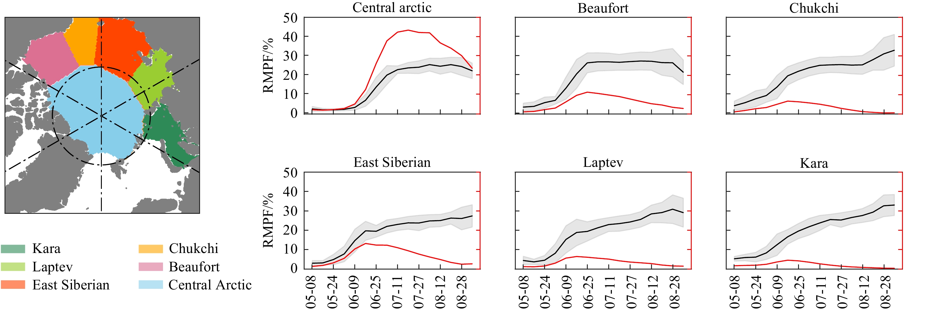
Figure 1b shows the changes of ponds at various latitudes in the Arctic over the past two decades, displaying significant latitudinal differences. Melt ponds appear first at lower latitudes, where MPA reaches its peak earlier. However, as the season progresses, MPA gradually decreases while RMPF gradually increases, resulting in low MPA and high RMPF in late July and early August at lower latitudes. Note that although melt ponds appear later at higher latitudes, they persist for a longer duration once they appear. Fig. 2 illustrates the seasonal evolution of ponds in different seas of the Arctic, the results show obvious differences in pond characteristics across different regions. The seasonal changes of ponds in the central area are very similar to the overall evolution in the Arctic. The start point of rapid growth period in the central zone is delayed by about 20 days compared to the marginal seas, but the total MPA peak can reach over 6 ×10⁵ km2, which is 4 to 5 times the peak of other seas. Moreover, the RMPF in the central area can maintain around 23% during the flat period, which is at least 5% lower than in other seas.
Figure
2.
The variation of melt ponds in various Arctic seas from 2002 to 2022.The black and red solid line represents RMPF and total MPA respectively, the gray shaded is the standard deviation of RMPF.
Over the past 20 years, the average RMPF in the Arctic has been (20.1±1.6%), with a total MPA of (0.86±0.07) million km2. RMPF shows a slight increasing trend, while total MPA shows a significant decreasing trend of 0.54 × 10⁴ km2/year. The trends of ponds show clear differences with latitude and melting dates. As shown in Fig. 3b, both RMPF and MPA exhibit a significant increasing trend in the early melting period, mainly related to the earlier onset of melting and the extension of the melting season in the Arctic region (Yang et al., 2022; Stroeve et al., 2014). Arctic summer ponds show distinctly different trends at higher and lower latitudes; MPA significantly decreases at lower latitudes with a slight change in RMPF, while both RMPF and MPA show increasing trends at higher latitudes.
Figure
3.
Inter-annual variation of melt ponds in the Arctic from 2002 to 2022. (a) the black and red solid line represents RMPF and total MPA respectively. The red dashed line indicates the linear trend, which passes the 95% significance test. The blue bar is SIT. (b) the inter-annual variation of RMPF and MPA with latitude, * indicates passing the 95% significance test.
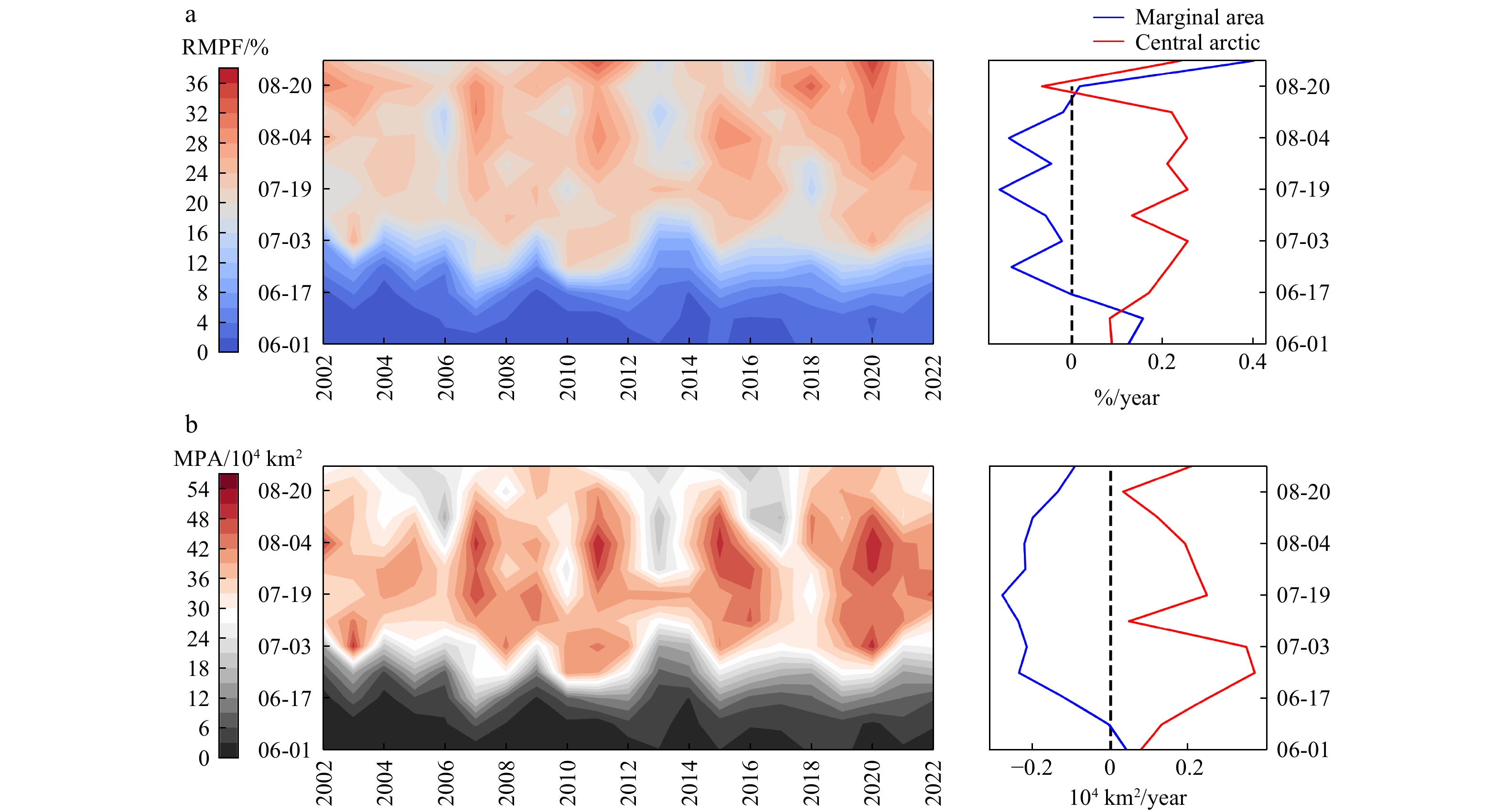
As known from Fig. 2, the total MPA peak in the central Arctic is 4-5 times higher than in the marginal seas, and the ponds changes in the central area almost dominate the overall evolution characteristics of Arctic ponds. Fig. 4 focuses on the evolution of melt ponds in the central area, with significant high pond coverage in years of anomalous sea ice melting such as 2007, 2011, 2015, and 2020. The phenomenon of increased ponds in the central Arctic and decreased ponds in the marginal seas appears almost throughout the summer, with the differences most pronounced from late June to early August. For example, on July 19, the trends of total MPA and RMPF in the central area increased by 0.25 × 10⁴ km2/year and 0.26%/year, respectively, while the trends in the marginal seas were −0.27 × 10⁴ km2/year and −0.16%/year, respectively. The increased ponds not only activate the local melt pond-shortwave radiation positive feedback mechanism (Perovich and Tucker III, 1997; Brandt et al., 2005), accelerating sea ice melting in thick ice areas, it also releases more latent heat during the freezing season, delaying sea ice growth (Flocco et al., 2015). Both have significant impacts on future climate change in the central Arctic.
Figure
4.
Distribution of summer ponds in the central Arctic from 2002 to 2022. (a) and (b) represent the distribution of RMPF and total MPA, respectively. The small graph on the right shows the trend of pond in the central arctic and marginal seas
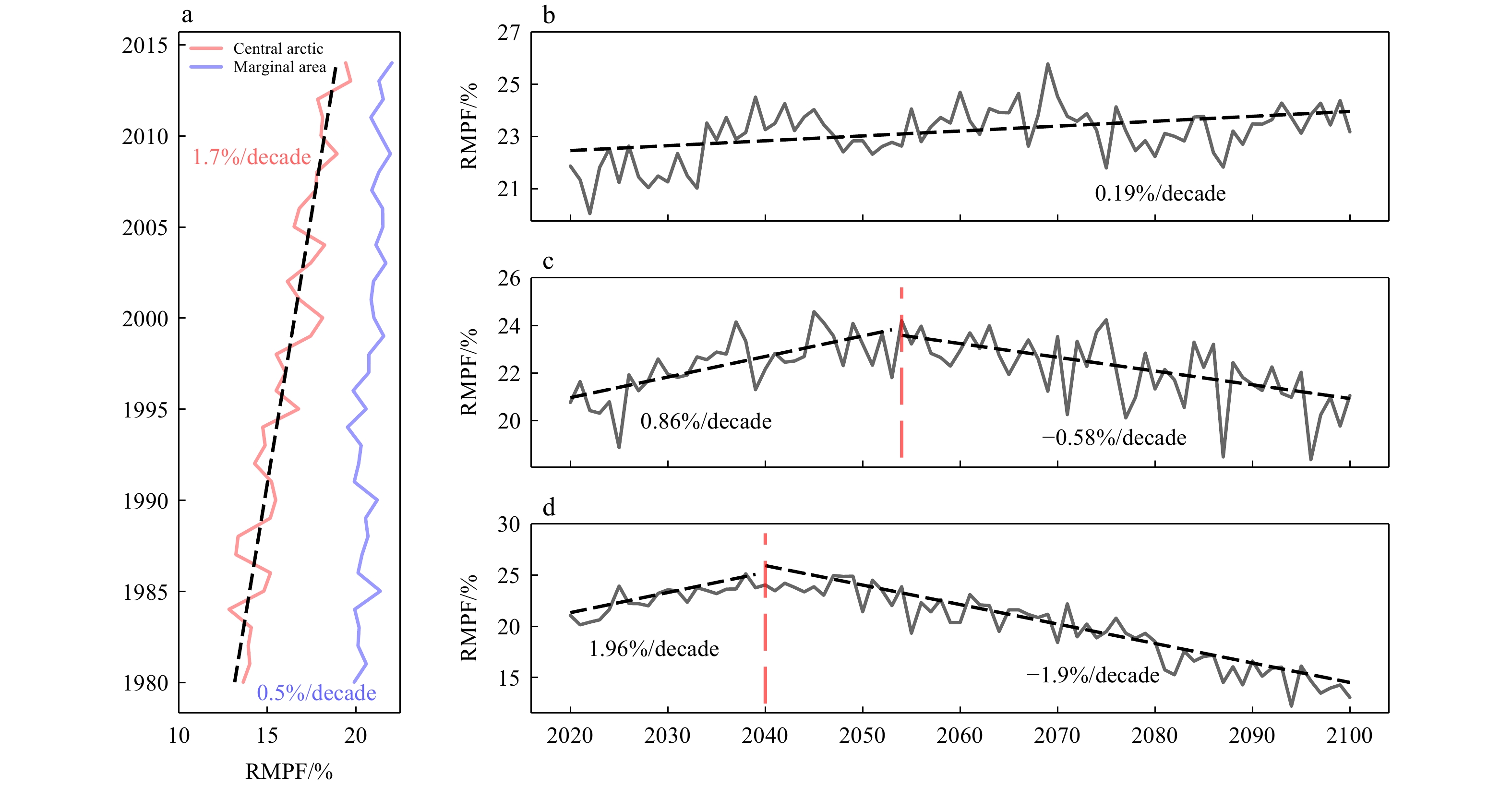
To further illustrate the interannual variations of melt ponds in the central region, we introduce pond data outputted by models in CMIP6. The results have shown in Fig. 5. Before analyzing future changes in melt ponds, we compared the historical simulations against remote sensing data, finding consistent interannual trends. Notably, since 1980, both the central Arctic and peripheral seas have exhibited significant growth trends, with the central region growing more than three times faster than the peripheral seas. This aligns with the observed increasing trend in the central region. Under different socio-economic emission scenarios, RMPF show clear differences. Under low emission scenarios, RMPF exhibits significant growth, but under SSP2-4.5 and SSP5-8.5 scenarios, RMPF shows a pattern of significant decrease following an initial increase. To confirm the turning points have statistical significance, we use the Mann-Kendall (MK) test combined with a sliding window method for turning point detection. First, we calculated the 30-year moving trends under medium and high emission scenarios, respectively. Second, we selected the first point where the trend shifts from positive to negative and passes the 99% significance test as the turning point (Fig. S1). In the medium emission scenario, RMPF displays a significant increasing trend before 2055, followed by a significant decreasing trend thereafter. In the high emission scenario with stronger radiation forcing, this turning point occurs around 2040.
Figure
5.
Average RMPF in the central Arctic under different CMIP6 emission scenarios (a) the SSP1-2.6 scenario, with the black solid line representing the change in RMPF and the black dashed line representing the linear trend that passes the 95% significance test. (b) and (c) are similar to (a) but correspond to the SSP2-4.5 and SSP5-8.5 scenarios, respectively.
As intermediates in ice-atmosphere interactions, melt ponds primarily depend on the state of sea ice and atmospheric conditions (Rösel and Kaleschke, 2012). Being products of surface melting, pond changes are inevitably closely linked to sea ice. Previous studies have highlighted the significant impact of ice type and surface topography on pond evolution. The rough surface topography of multi-year ice tends to limit the extent of pond coverage, while the smoother surface of first-year ice often allows for higher levels of coverage (Roeckner et al., 2012; Polashenski et al., 2012). The carrying capacity for melt ponds varies significantly with the thickness of the underlying sea ice, and in the following we will analyze the relationship between pond changes and sea ice thickness.
The distribution of summer ponds with SIT, as shown in Fig. 6, indicates that both RMPF and MPA decrease with the increasing SIT in June. Two peaks are observed that one in the thin ice zone of 0.6m-0.8m and another in the thicker ice zone of 1.8-2.2m, corresponding to the two peaks in RMPF distribution. During this rapid growth period, the pond coverage gradually spreads from the thin ice zone to the thicker ice zone. In July and August, a slight decrease in RMPF and significant increase in MPA with increasing SIT are observed. This is because the denser ice cover leads to a decrease in RMPF although there is larger pond area. Observations and model results by Webster et al. also indicate that RMPF on multi-year ice is lower than that on first-year ice (Webster et al., 2015).
Figure
6.
Distribution of summer RMPF and MPA and their relationship with SIT. (a)(b) represent the average RMPF distribution and their relationship with SIT for June, the marginal bar showing the density distribution of SIT and RMPF in different areas. (c)(d) follow the same format but for MPA. e, f, g, h; i, j, k, l is similar to a, b, c, d but for July and Aug respectively.
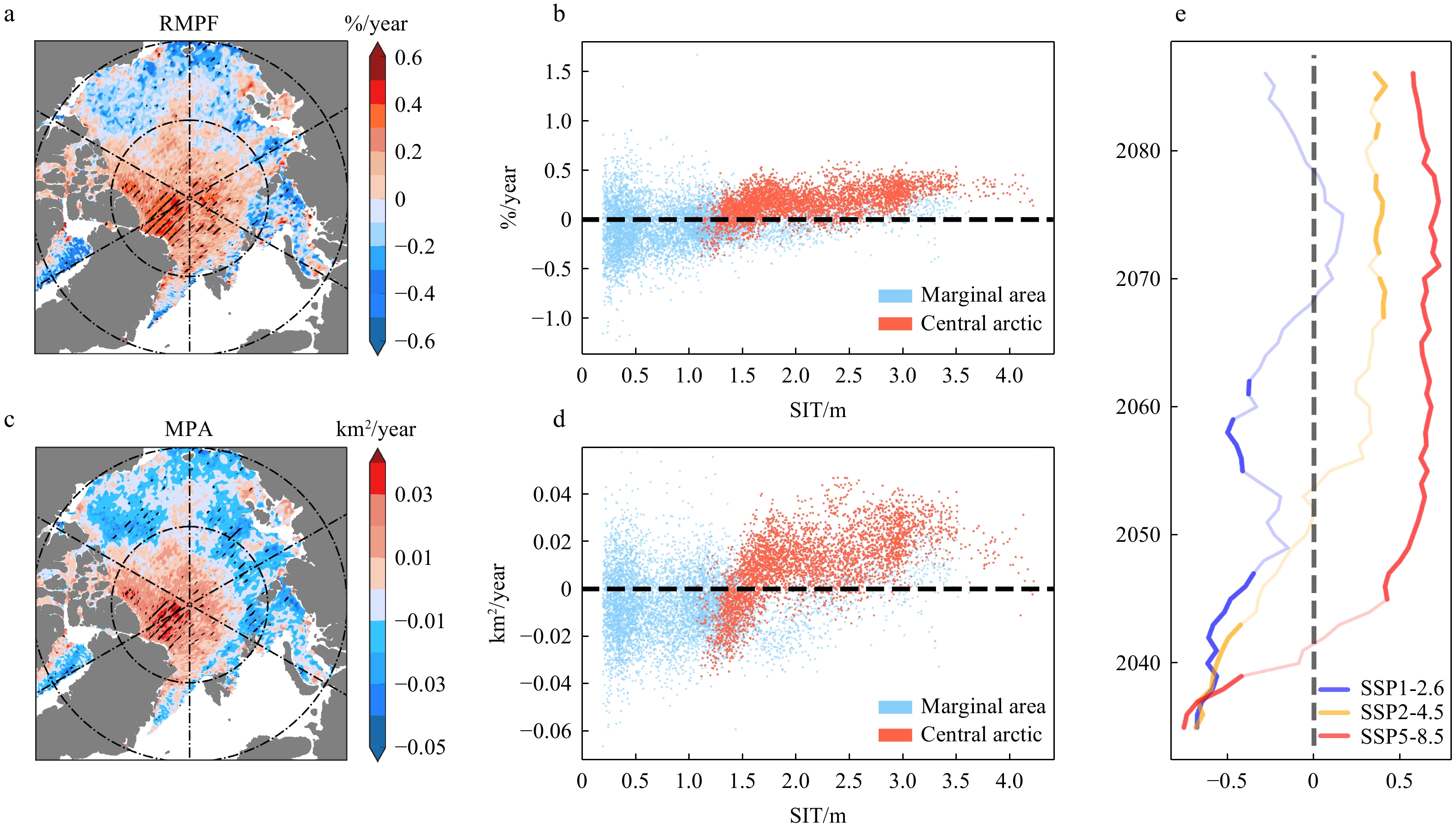
In recent 20 years, the MPA in the marginal seas has significantly decreased, primarily due to the drastic reduction of sea ice in these areas, leading to a weakened or even vanished capacity to support ponds. In contrast, in the central Arctic, the sea ice is predominantly thicker multi-year ice, with an average summer sea ice thickness of over 1.5 m (Fig. 7). The sea ice state is usually more stable than marginal seas and its capacity to support ponds relatively strengthens against the backdrop of Arctic warming and ice melting. Therefore, both RMPF and MPA show increasing trends. Especially, significant growth of ponds is observed in north of Greenland, which is consistent with the previous conclusions (Feng et al., 2022). The above phenomena can be further validated by calculating the 30-year moving correlation coefficient between detrended RMPF and SIT in the central region under different emission scenarios. When the thickness is substantial, there is a negative correlation between SIT and RMPF, with RMPF increasing as SIT decreases. However, when SIT decreases to a certain threshold, the correlation between SIT and RMPF becomes positive, with RMPF decreasing as sea ice melts. The thresholds under SSP2-4.5 and SSP5-8.5 scenarios are 1.73m and 1.88m, respectively. The variation in SIT and its capacity to support melt ponds is a key reason for the significant difference in pond trends.
Figure
7.
Spatial distribution of summer pond trends and their relationship with sea ice thickness including the period spanning 2002-2022. (a) The spatial distribution of the RMPF trends. (b) The relationship between RMPF and SIT. The red and blue dots represent central arctic and marginal area, respectively. (c) and (d) are similar to (a) and (b) but for MPA. (e)The 30-year moving-correlation between RMPF and SIT in the central region under different future emission scenarios, with the bold solid line indicating parts that pass the 95% significance test.
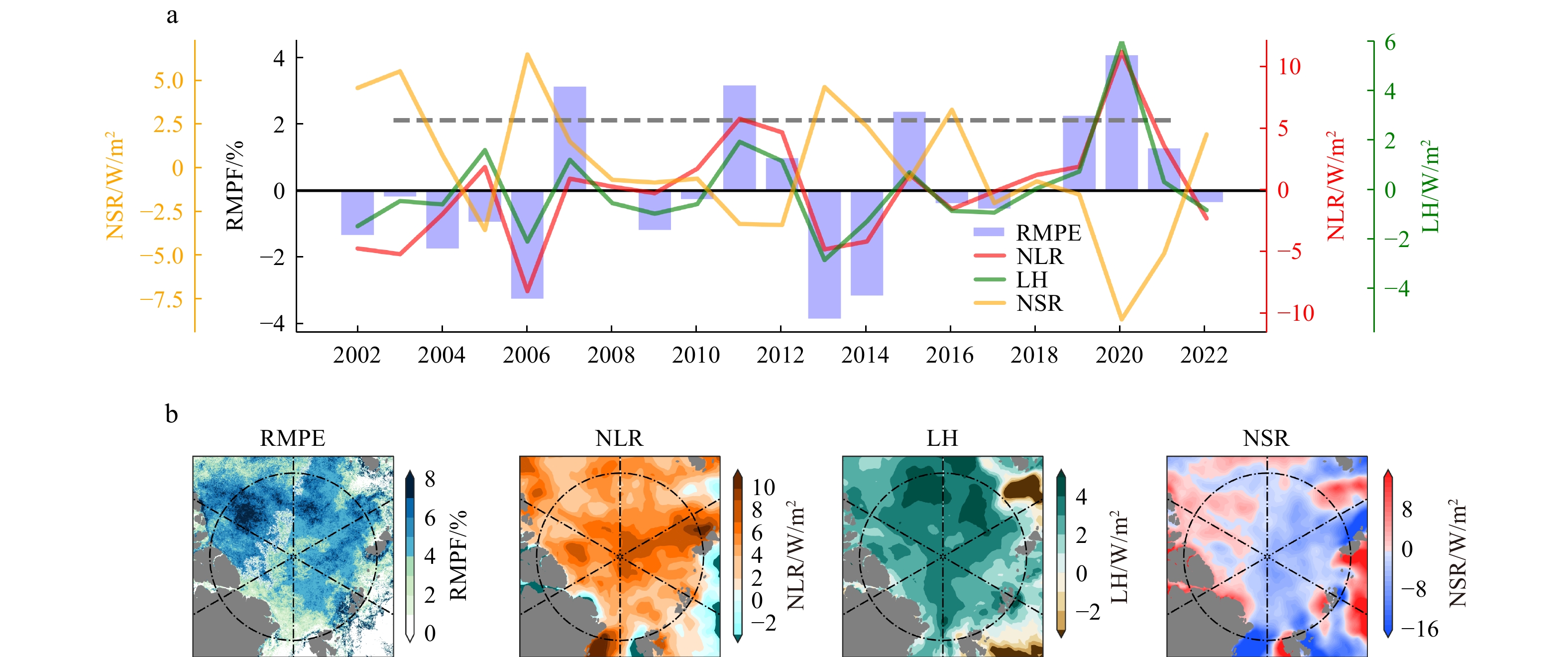
Melt ponds exposed directly to the air are primarily controlled by ice-atmosphere energy exchange when the carrying capacity of the sea ice does not change significantly. Table 2 shows the correlation coefficients between pond anomalies and atmospheric energy flux anomalies in the central Arctic. Before calculating the correlation coefficients, trends in all variables were removed. The correlation between NLR, LH anomalies and RMPF anomalies is as high as 0.8, while the NSR anomalies show a significant negative correlation. Although NSR flux is the main source of surface energy in the Arctic summer, the pond changes in the entire central Arctic are controlled by NLR and LH. Fig. 8 further illustrates their connection, with widespread positive anomalies of NLR and LH flux and negative anomalies of NSR in years of high pond anomalies in the central Arctic. However, it is noteworthy that under the local pond-shortwave radiation positive feedback mechanism, larger positive anomalies of melt ponds correspond to positive anomalies of NSR.
Table
2.
Correlation between melt ponds and various influencing factors anomalies in the central Arctic from 2002 to 2022. Bold and * indicate passing the 95% significance test.
Figure
8.
The connection between summer ponds and energy flux anomalies in the central Arctic from 2002 to 2022 (a) the inter-annual anomalies of RMPF, LH, NLR and NSR. The grey dashed line represents the standard deviation of RMPF. (b) The composite distribution of RMPF, NLR, LH, NSR anomalies.
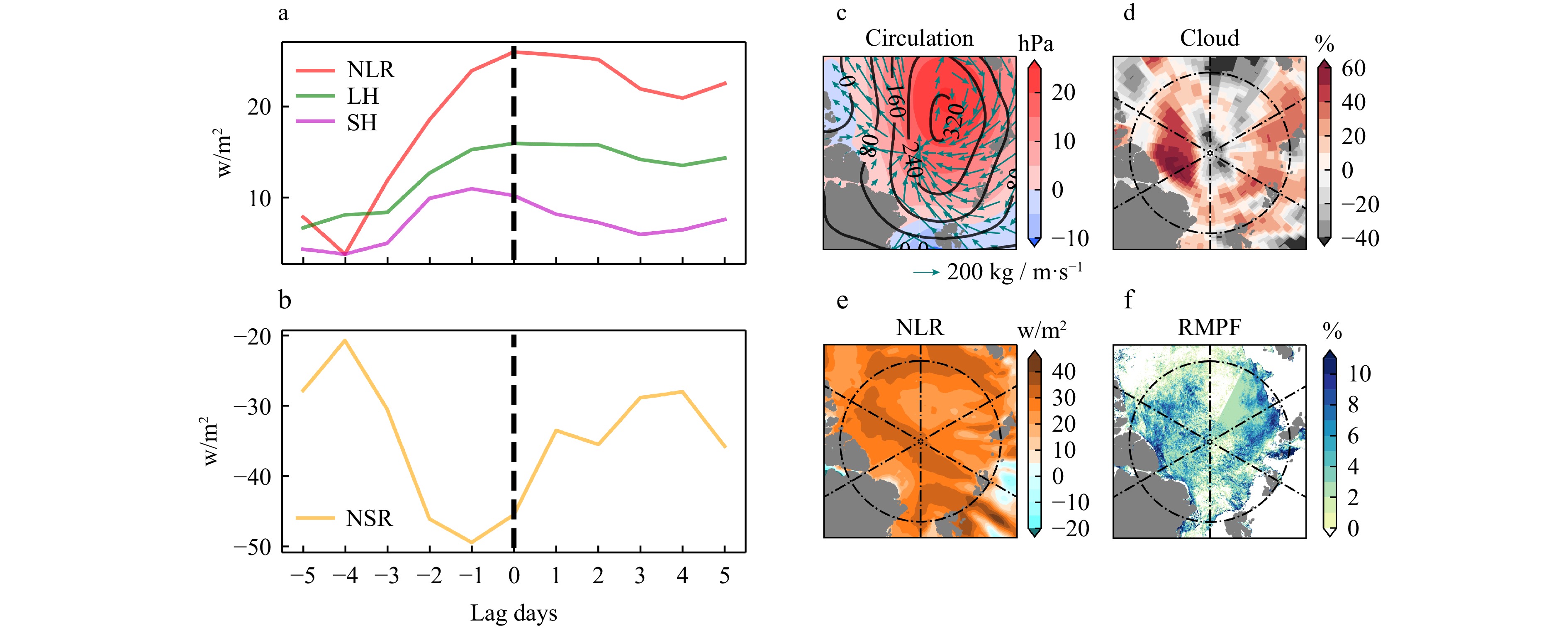
Taking a significant positive anomaly event of ponds in the central area as an example, Fig. 9 displays the corresponding atmospheric variable anomalies on July 11, 2020. In the early stages before the event, there is often a continuous increase in positive anomalies of NLR and LH fluxes along with negative anomalies of NSR. From 4 days before the event to its occurrence, the positive anomaly of NLR increased by 22.2 w/m2, and the positive anomalies of LH and SH fluxes increased by 7.86 w/m2 and 6.47 w/m2, respectively, while the negative anomaly of NSR increased by −24.78 w/m2. Additionally, it is evident that during this anomalous pond event, the central Arctic was dominated by a large, highly barotropic anticyclonic circulation anomaly. The center SLP and 500hPa geopotential height anomaly reached up to 25hPa and 320gpm, respectively. This powerful anticyclonic anomaly transported a significant amount of water vapor from the Atlantic sector to the central Arctic, resulting in positive anomalies in low cloud cover, NLR, and LH. Consequently, this led to an increase in surface temperature, enhanced melting of sea ice, and a positive anomaly in melt ponds. The anomalies of them correspond well with the pond anomalies, further underscoring the significance of DLR and LH at the weather scale in increasing sea ice melt and melt pond coverage. The similar phenomenon occurred in other cases on Aug 5, 2007 (Fig. S2). The exceptional sea ice melting closely linked to NLR and LH anomalies has also been reflected in other studies. Kapsch et al. have demonstrated that in years with significantly lower sea ice extent than normal have stronger NLR and turbulent flux in springtime, while downward shortwave radiation plays a role in feedback amplification after the onset of melting (Kapsch et al., 2013). Wang et al. suggests that enhanced DLR tied to the warm, moist air mass transport plays an important role in large daily sea ice loss event over the all arctic, although NSR do not seem to affect it significantly (Wang et al., 2020).
Figure
9.
Changes in atmospheric variable anomalies during the positive melt pond event on July 11, 2020. (a)(b) The energy flux anomaly of the lag days. (c) The shade and black line indicates the SLP anomaly and 500hPa geopotential height anomaly, respectively. The vector indicates that the integrated moisture transport. (d−f) The low cloud cover anomaly, the NLR anomaly and RMPF anomaly respectively.
This study employs the latest satellite data and multi-model averaged outputs from CMIP6 to systematically analyze the spatiotemporal evolution characteristics of Arctic melt ponds and their relationship with SIT and atmospheric energy flux. We have derived some interesting conclusions summarized as follows:
The study examines changes in melt ponds using both the relative melt pond fraction (RMPF) and absolute melt pond area (MPA). Melt ponds initially form in the lower latitude marginal seas, where MPA increases and then decreases as the season progresses, while RMPF gradually increases. The peak MPA in the central Arctic can exceed 0.6 million km2, which is 4 to 5 times that of other marginal seas. Over the past two decades, the Arctic's RMPF has slightly increased, while MPA has shown a significant annual decline of 0.54×10⁴ km². Additionally, summer ponds show distinctly different trends at different latitudes; lower latitudes experience a significant decrease in MPA and minor changes in RMPF, while higher latitudes see increases in both RMPF and MPA. Both satellite retrieval data and CMIP6 model outputs indicate that the ice thickness and corresponding support capacity is the key reason for the significant difference. The drastic reduction of sea ice in the marginal seas over recent decades, reducing or even eliminating their capacity to support ponds, leading to a decrease in pond coverage. In contrast, in the central Arctic, where the sea ice state is more stable and melting periods have lengthened, there is a significant increase. Beyond the carrying capacity of sea ice, the overall pond variations are influenced and controlled by the flux of NLR and LH on the central arctic. The correlation between NLR, LH anomalies and RMPF anomalies is as high as 0.8, while the NSR anomalies show a significant negative correlation. This is closely linked to the unusual atmospheric circulation patterns, which transported a significant amount of water vapor to the center area, resulting in positive anomalies in low cloud cover, NLR, LH and negative anomalies in NSR. Therefore, changes in melt ponds across the central Arctic are primarily influenced by NLR and LH. The pond-shortwave positive feedback occurs locally only under stable atmospheric circulation and clear weather conditions.
To ensure the reliability of our conclusions, we also utilized melt pond datasets retrieved by Ding et al. and Rosel et al. Due to the shorter duration of Rosel et al.'s data, changes in the RMPF were not very pronounced. However, Ding et al.’s dataset, which spans from 2001 to 2019, exhibited a consistent trend with our findings. We also examined the impact of different sources of thickness data on the uncertainty of our results. Both satellite and PIOMAS product revealed a similar spatial pattern of SIT, reinforcing the reliability of our conclusions in section 3.2. Notably, PIOMAS tends to significantly overestimate SIT in the northern part of Greenland by more than 0.5 meters. This overestimation might introduce uncertainties when discussing the relationship between SIT and other variables, which is not our primary focus. Although satellite data with higher spatial and temporal resolution can help us delve deeper into the overall evolution characteristics of Arctic ponds, inevitable errors in satellite retrieval technology, such as the identification of bare ice and snow, often increase the uncertainty (Xiong and Ren, 2023). The development and evaluation of more accurate in-situ observations, satellite retrieval, and diverse pond datasets are crucial for understanding this important physical process in the future (Ding et al., 2020; Wright and Polashenski, 2020).
Acknowledgements:
We are also very grateful for the data provided by A.P. Chuan Xiong.
Xu Fang, Lujun Zhang. The evolution characteristics and causes of melt ponds in the Arctic Ocean[J]. Acta Oceanologica Sinica. doi: 10.1007/s13131-024-2390-z
Xu Fang, Lujun Zhang. The evolution characteristics and causes of melt ponds in the Arctic Ocean[J]. Acta Oceanologica Sinica. doi: 10.1007/s13131-024-2390-z
Table
2.
Correlation between melt ponds and various influencing factors anomalies in the central Arctic from 2002 to 2022. Bold and * indicate passing the 95% significance test.
Figure 1. The evolution of melt ponds in the Arctic region from 2002 to 2022. (a) The RMPF and MPA change with SIT, the gray shaded is the standard deviation of RMPF. The dashed line and spatial map show the RMPF evolution in 2007. (b) the variation of RMPF and MPA with latitude.
Figure 2. The variation of melt ponds in various Arctic seas from 2002 to 2022.The black and red solid line represents RMPF and total MPA respectively, the gray shaded is the standard deviation of RMPF.
Figure 3. Inter-annual variation of melt ponds in the Arctic from 2002 to 2022. (a) the black and red solid line represents RMPF and total MPA respectively. The red dashed line indicates the linear trend, which passes the 95% significance test. The blue bar is SIT. (b) the inter-annual variation of RMPF and MPA with latitude, * indicates passing the 95% significance test.
Figure 4. Distribution of summer ponds in the central Arctic from 2002 to 2022. (a) and (b) represent the distribution of RMPF and total MPA, respectively. The small graph on the right shows the trend of pond in the central arctic and marginal seas
Figure 5. Average RMPF in the central Arctic under different CMIP6 emission scenarios (a) the SSP1-2.6 scenario, with the black solid line representing the change in RMPF and the black dashed line representing the linear trend that passes the 95% significance test. (b) and (c) are similar to (a) but correspond to the SSP2-4.5 and SSP5-8.5 scenarios, respectively.
Figure 6. Distribution of summer RMPF and MPA and their relationship with SIT. (a)(b) represent the average RMPF distribution and their relationship with SIT for June, the marginal bar showing the density distribution of SIT and RMPF in different areas. (c)(d) follow the same format but for MPA. e, f, g, h; i, j, k, l is similar to a, b, c, d but for July and Aug respectively.
Figure 7. Spatial distribution of summer pond trends and their relationship with sea ice thickness including the period spanning 2002-2022. (a) The spatial distribution of the RMPF trends. (b) The relationship between RMPF and SIT. The red and blue dots represent central arctic and marginal area, respectively. (c) and (d) are similar to (a) and (b) but for MPA. (e)The 30-year moving-correlation between RMPF and SIT in the central region under different future emission scenarios, with the bold solid line indicating parts that pass the 95% significance test.
Figure 8. The connection between summer ponds and energy flux anomalies in the central Arctic from 2002 to 2022 (a) the inter-annual anomalies of RMPF, LH, NLR and NSR. The grey dashed line represents the standard deviation of RMPF. (b) The composite distribution of RMPF, NLR, LH, NSR anomalies.
Figure 9. Changes in atmospheric variable anomalies during the positive melt pond event on July 11, 2020. (a)(b) The energy flux anomaly of the lag days. (c) The shade and black line indicates the SLP anomaly and 500hPa geopotential height anomaly, respectively. The vector indicates that the integrated moisture transport. (d−f) The low cloud cover anomaly, the NLR anomaly and RMPF anomaly respectively.


 DownLoad:

 DownLoad: