Figure
1.
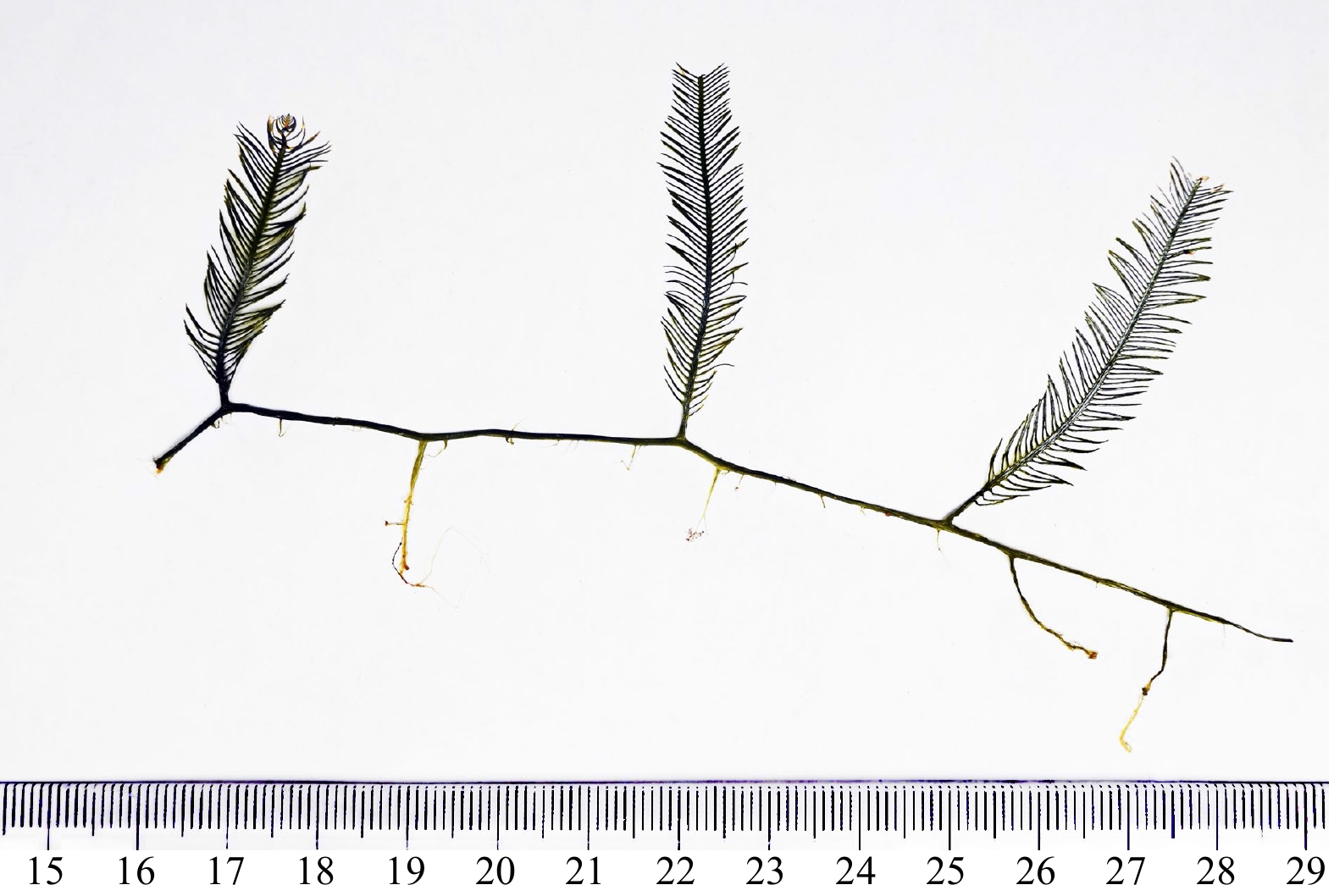
The external morphology of Caulerpa sertularioides.
| Citation: | Lei Ren, Lingna Yang, Yaqi Wang, Peng Yao, Jun Wei, Fan Yang, Fearghal O’Donncha. Forecasting of surface current velocities using ensemble machine learning algorithms for the Guangdong−Hong Kong−Macao Greater Bay area based on the high frequency radar data[J]. Acta Oceanologica Sinica, 2024, 43(10): 1-15. doi: 10.1007/s13131-024-2363-2

|
Caulerpa is a genus of marine green algae distributed mainly in tropical and subtropical waters and has more than 90 species. The thalli contain caulerpin, an alkaloid extracted from Caulerpa. The compound has anti-inflammatory activity, is rich in minerals and vitamins (Jiang et al., 2011), and has great value in application in the industries of food (de Gaillande et al., 2017), medicine (Gao, 2014; Chaves Filho et al., 2022), high-grade fertilizer (Wang, 2010), energy (Huang, 2012), and bioremediation of marine waters (Landi et al., 2022). Physiological and ecological studies have mostly focused on some environmental factors such as temperature (Li et al., 2022; Shi et al., 2022), salinity (Guo et al., 2015; Cai, 2021), irradiances (Stuthmann et al., 2021; Zhong et al., 2021), nutrient (Liu et al., 2016; Zhang et al., 2020) and heavy metal salt stress (Pang et al., 2021) for cultivated Caulerpa lentillifera in Southeast Asian countries. However, due to invasive nature, some species caused ecological problems in the Mediterranean, America, Australia, and other waters in the world (Davis et al., 1997; Meinesz et al., 2001; Verlaque et al., 2004; Anderson, 2005; Lapointe et al., 2005; Klein and Verlaque, 2008; Kang et al., 2021). In a eutrophic sea where some species boom excessively, vast and thick algal mats would form on the seafloor, which hamper sunlight transmission and seawater exchange, posing a large threat to local mariculture activities or coral reef growth (Williams and Schroeder, 2004). In environments with poor water quality, these blooming species have a strong ability to absorb nutrients from water and sediments (Williams, 1984; Kolar and Lodge, 2001). Therefore, they have the potential for sewage treatment (Landi et al., 2022).
Some of the Caulerpa species are highly invasive such as Caulerpa taxifolia and Caulerpa racemosa (Anderson, 2005; Fernández and Cortés, 2005; Liu et al., 2019). Caulerpa sertularioides (Anderson, 2005; Fernández and Cortés, 2005), also known as green feather alga, is similar in appearance and has the same mode of reproduction as C. taxifolia, including well-developed stolons and rhizoids for easy attachment to substrates (Fig. 1). It is highly invasive because its fragment of stolons can grow continuously from its apices (Smith and Walters, 1999), and spread quickly in the tropical northeast Pacific (Withgott, 2002). Its bloom damaged the coral reefs seriously (Smith et al., 2010). Some scientists believed that the high invasion ability might be related to a favorite temperature and the quick proliferation of thallus fragments (Fernández and Cortés, 2005). Some affected countries (such as Spain and France) are very concerned about the invasion and have tried to eradicate or control it by banning the trade of aquatic species (Klein and Verlaque, 2008).
In China, C. sertularioides was distributed mainly along the coast of the South China Sea in Taiwan, Hainan, and other islands (Ding et al., 2015; Liu et al., 2019). During the growing season, its blooms and the biomass abounds along the coast of the South China Sea (Fig. 2). However, few previous studies focused on its antimicrobial activities (Kumar et al., 2011), and polysaccharides and sterols (Shevchenko et al., 2009; Chaves Filho et al., 2022). More studies are required to elucidate its invasion characteristics and potential.

The response surface methodology (RSM) is a new statistical method for solving multivariable problems and exploring optimal process parameters by analyzing the regression equation (Mee, 2009; Mäkelä, 2017). It has been widely used in the research of life science in recent years because of its advantage of direct display selection of optimal operating conditions in experiment design (Kim et al., 2019; Srinivas et al., 2019; Faramarzi et al., 2019; da Silva et al., 2019; Vishwakarma and Banerjee, 2019; Ebadi et al., 2019; Nur et al., 2019). In China, the RSM method has recently been used to analyze the algal polysaccharides of Caulerpa lentillifera, demonstrating its advantages in the analysis of the active ingredients of algae (Tong et al., 2022).
In this study, effects of irradiance, temperature, and salinity on the growth of C. sertularioides are studied by using RSM. By determining and analyzing the optimum conditions of multiple ecological factors, it will provide reasonable data for cultivation, prevention and control of biological invasion of C. sertularioides in the natural waters.
The samples of C. sertularioides were bought from Tianjin’s aquariums and pre-cultured for one week in a seawater tank at room temperature, the thalli were washed and cleaned with disinfected seawater to remove debris, and then cultured under aeration for 30 days under the conditions of irradiance (37.5 ± 6.25) μmol/(m2·s), temperature (25 ± 1)℃, and salinity (30 ± 1) to obtain adequate biomass for the following experiment.
The thalli with long stolons were picked out and cut with sterilized scissors into at least 3 cm-long fragments carefully, making sure each fragment containing some blades and rhizoids (Smith and Walters, 1999), and placed in the air for 15 s for better wound healing. The fresh weight of each fragment was between 0.31–0.38 g (the mean standard deviation was (0.35 ± 0.02) g).
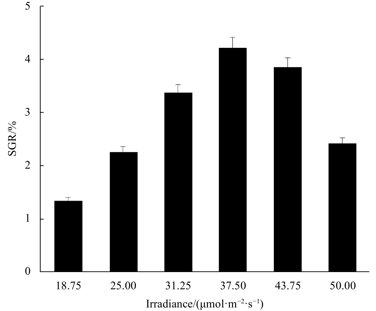
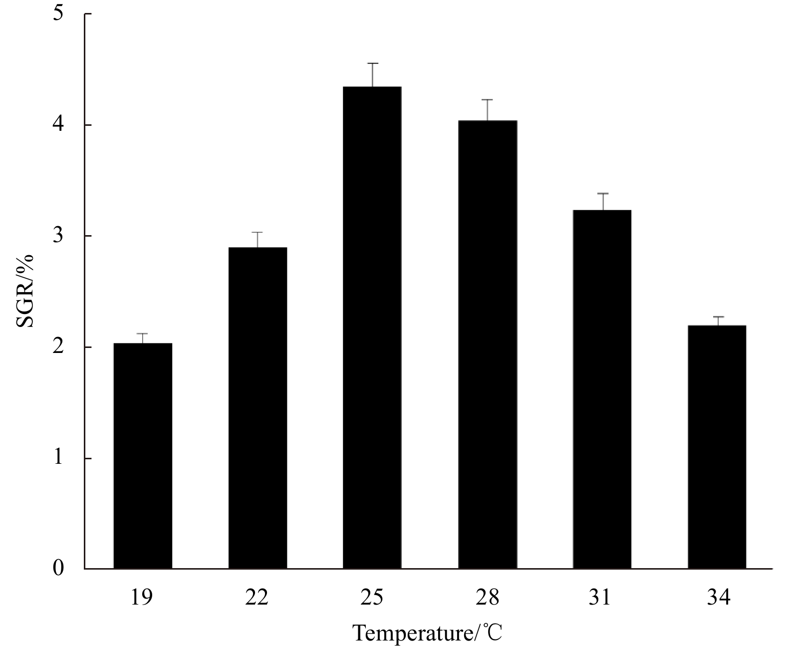
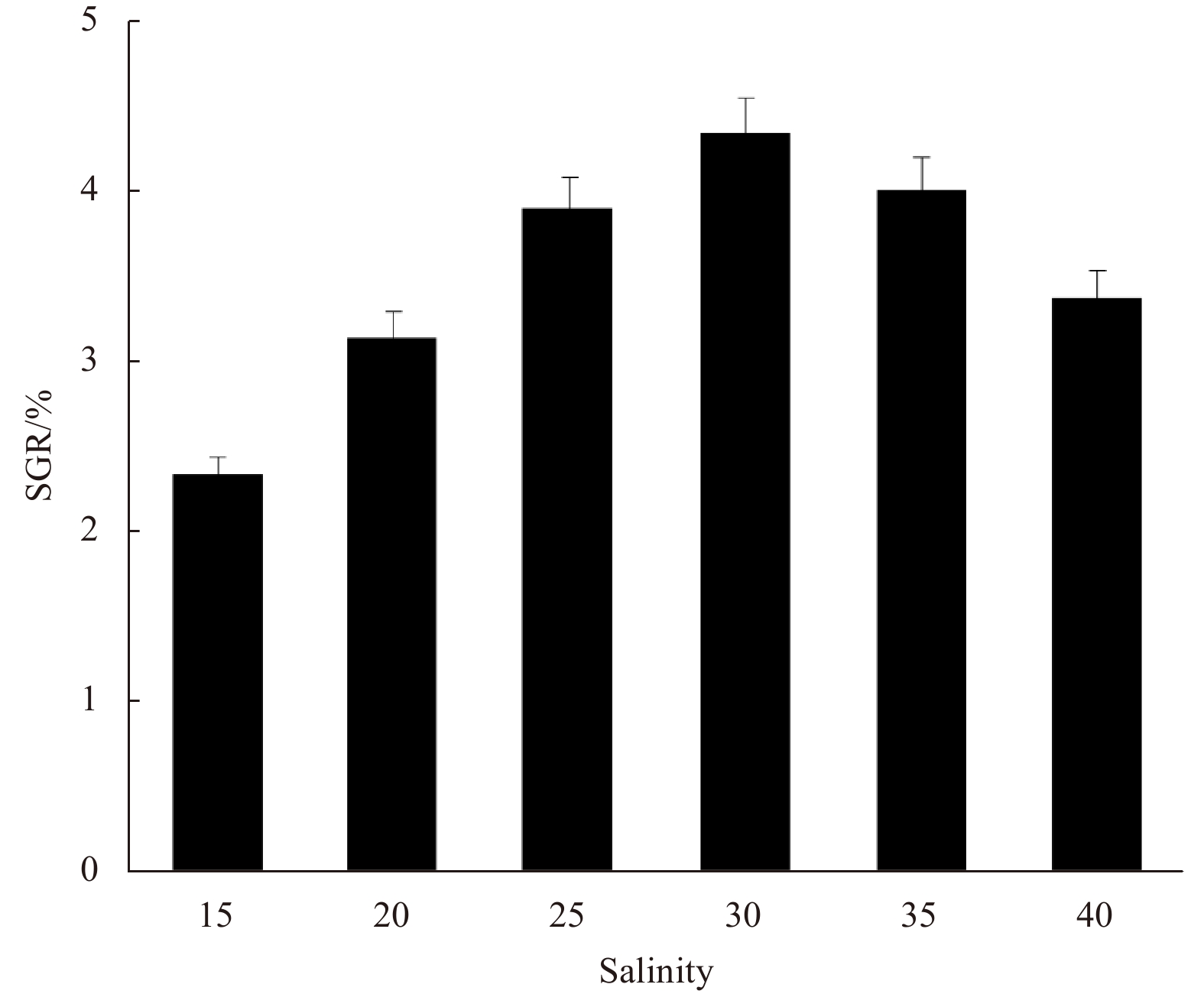
Referring to the cultivation experience and data, three ecological single-factor experiments, in which three main factors, e.g., irradiance, salinity, and temperature are tested and each is assigned a variable value, while the other two are constants. The conditions were set as: (1) irradiance at 18.75 μmol/(m2·s), 25.00 μmol/(m2·s), 31.25 μmol/(m2·s), 37.50 μmol/(m2·s), 43.75 μmol/(m2·s) and 50.00 μmol/(m2·s), salinity at 30 and temperature at 25℃; (2) temperature at 19℃, 22℃, 25℃, 28℃, 31℃ and 34℃, irradiance at 37.5 μmol/(m2·s) and salinity at 30; and (3) salinity at 15, 20, 25, 30, 35 and 40, irradiance at 37.5 μmol/(m2·s) and temperature at 25℃.
Each sample (including three fragments) was placed in a 250 mL conical flask containing 200 mL seawater that was renewed daily and cultured in the thermostatic illumination incubator (Jiangnan Instrument Co., Ltd., Ningbo, type GXZ) referring to the different treatments above. The total cultivation cycles last a week. Each treatment group was replicated three times. All samples were taken out and weighted wet at the end of the week, and then the SGR (specific growth rate) was calculated.
A central combination design experiment and the verification experiment on the results of the RSM of the three factors were performed using multi-factor experimental method. The results of the single-factor experiment were used to confirm the horizontal range of the ecological factor. The Box-Behnken central combination design, or the Box-Behnken design for simplicity—an RSM method was used to determine the SGR of the thalli fragments, and the optimum conditions of irradiance, temperature, and salinity.
The experimental data were statistically analyzed using Design-Expert 10.
SGR can be expressed as:
| $$ {\rm{ SGR}} =\frac{W_t-W_0}{t} \times 100 \%, $$ | (1) |
where W0 is the fresh mass (g) of fragments at the initial stage; Wt is the fresh mass (g) of fragments at the end of the experiment; and t is the number of days of the experiment.
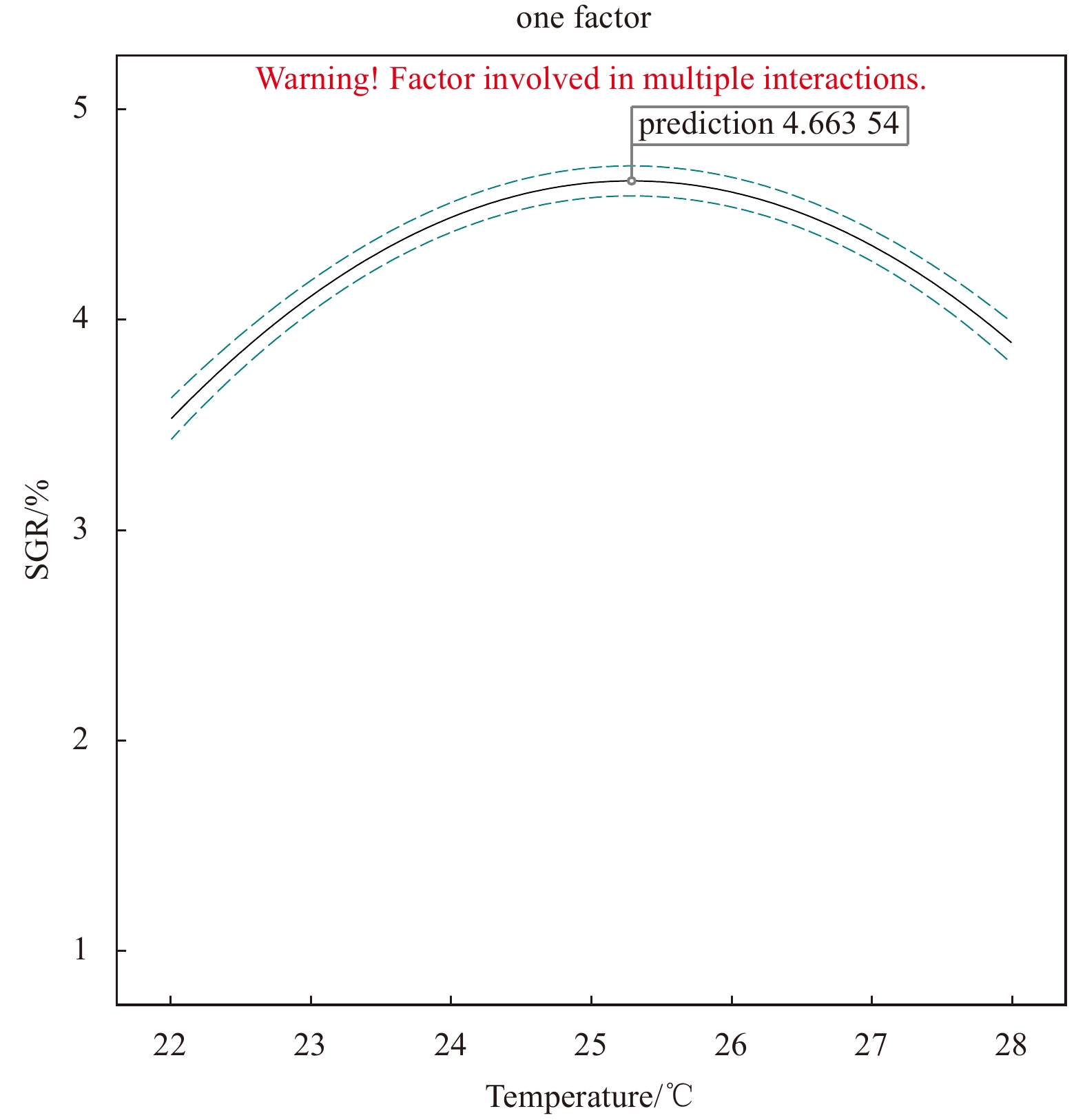
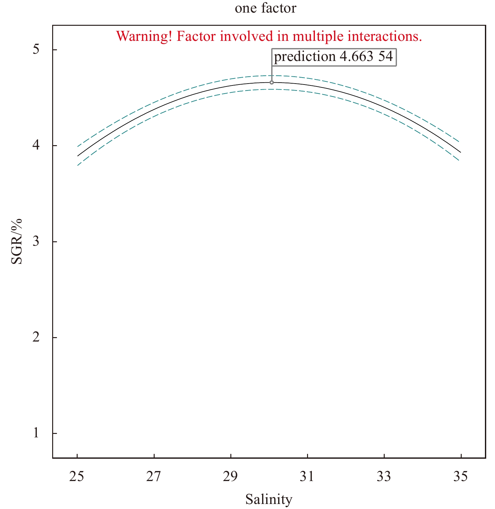
SGR of the fragments increased at first and then decreased with the increase of the variable factor. Peaks appeared at irradiance 37.5 μmol/(m2·s), temperature 25℃, and salinity 30, under which the SGR was 4.35%, 4.22%, and 4.33%, respectively (Figs 3–5).
Irradiance, temperature, and salinity are considered the three key factors affecting the growth of the species, and SGR is the response value. According to the results of the single-factor experiments, the horizontal ranges of the three factors were set and analyzed in the Box-Behnken design (Table 1), in which 17 three-factor combinations were determined and the SGRs of thalli fragments of the 17 combinations were measured (Table 2).
| Factor | Irradiance /(μmol·m−2·s−1) | Temperature/℃ | Salinity |
| Low | 31.25 | 22 | 25 |
| High | 43.75 | 28 | 35 |
 DownLoad:
CSV
DownLoad:
CSV
| Serial number | Irradiance/ (μmol·m−2·s−1) | Temperature/℃ | Salinity | SGR/% |
| 1 | 37.5 | 22 | 35 | 2.84 |
| 2 | 37.5 | 25 | 30 | 4.62 |
| 3 | 37.5 | 28 | 35 | 3.06 |
| 4 | 37.5 | 25 | 30 | 4.52 |
| 5 | 37.5 | 22 | 25 | 2.46 |
| 6 | 43.75 | 28 | 30 | 3.25 |
| 7 | 31.25 | 22 | 30 | 1.93 |
| 8 | 37.5 | 25 | 30 | 4.52 |
| 9 | 43.75 | 22 | 30 | 3.20 |
| 10 | 31.25 | 28 | 30 | 2.65 |
| 11 | 43.75 | 25 | 25 | 3.41 |
| 12 | 37.5 | 25 | 30 | 4.70 |
| 13 | 31.25 | 25 | 35 | 2.63 |
| 14 | 37.5 | 28 | 25 | 3.26 |
| 15 | 31.25 | 25 | 25 | 2.38 |
| 16 | 43.75 | 25 | 35 | 3.38 |
| 17 | 37.5 | 25 | 30 | 4.62 |
DownLoad:
CSV
Design-Expert 10 was used for the quadratic multiple regression of the data shown in Table 2. The regression equation was established as below:
| $$ \begin{aligned}{\rm{SGR}}(\%)= &\;4.60+0.46A+0.22B+0.049C-0.17AB-0.074AC-\\&0.14BC-0.90A^2-0.94B^2-0.75C^2, \end{aligned} $$ | (2) |
where A is irradiance, B is temperature, and C is salinity. The influences of factors A and B were highly significant (P < 0.000 1), and those of factors AB and BC were extremely significant (P < 0.01).
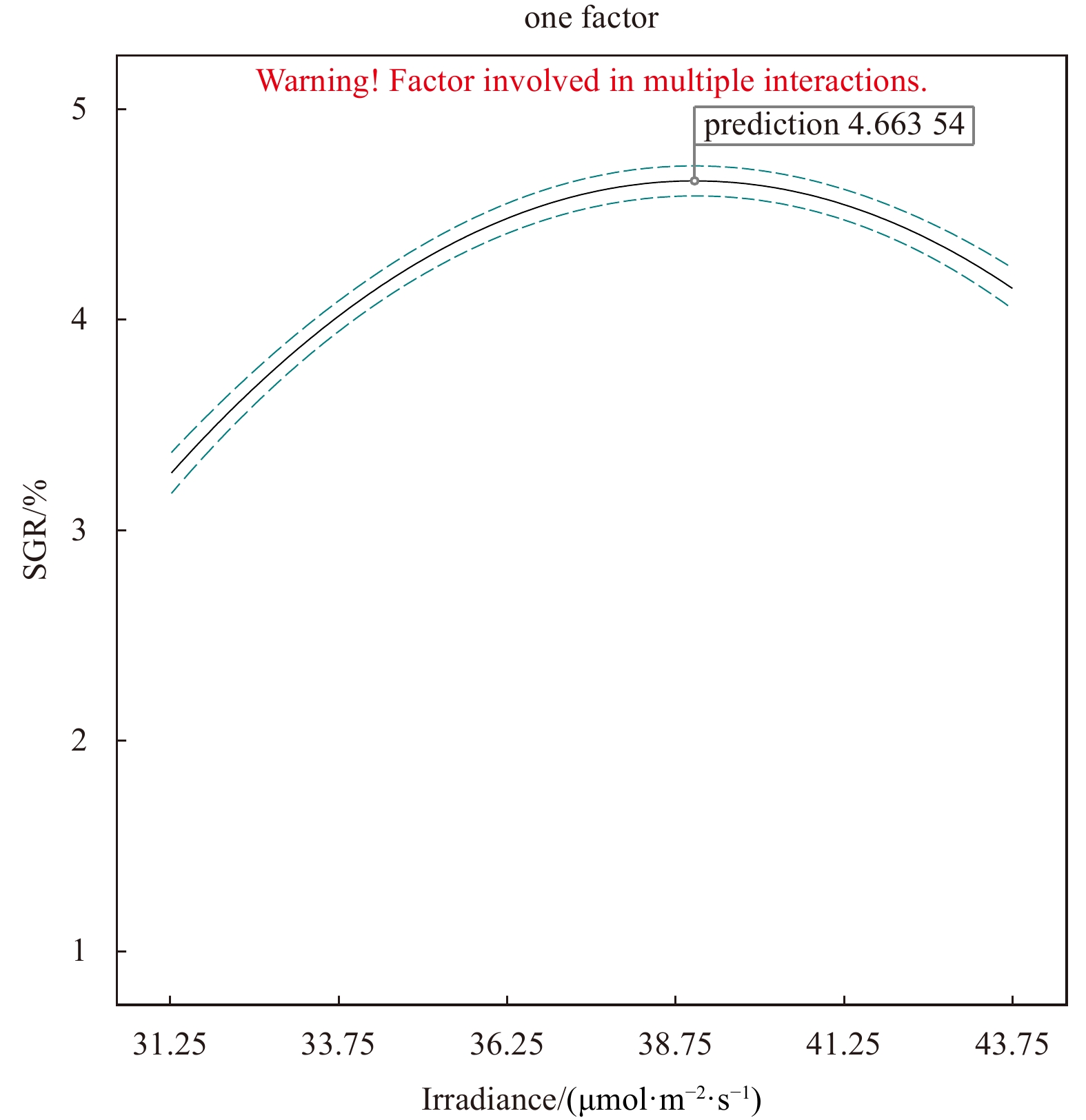
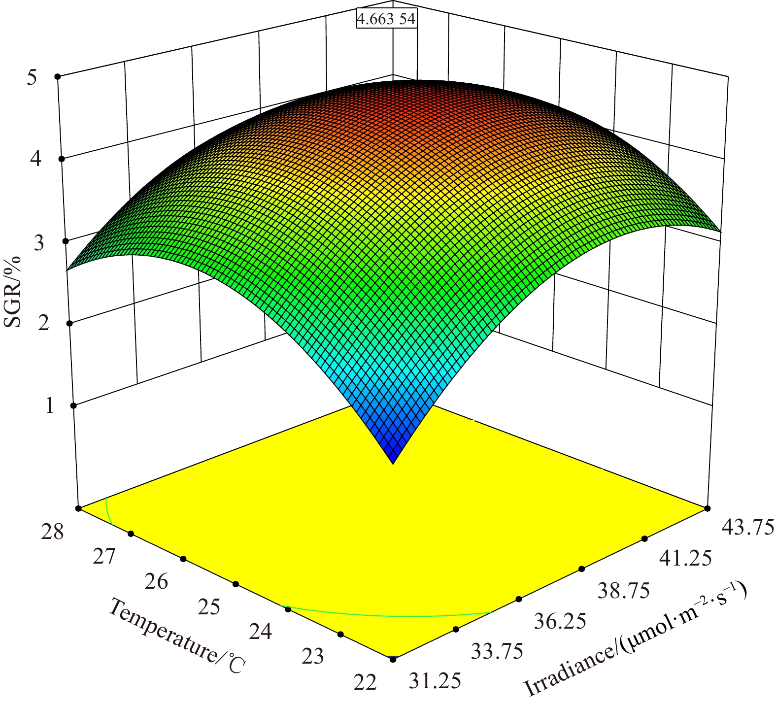
In addition, as ANOVA results show, the model of regression equation was highly significant (P < 0.000 1), while the lack-of-fit was not significant (P > 0.05), thus the mode could better describe the real relationship between various factors and the response value (SGR) (Table 3). In our response surface analysis (Figs 6–11), the factors involved in multiple interactions were irradiance (in μmol/(m2·s)), temperature (℃), and SGR (%). The results show that within the set range, the SGR of the fragments increased first and then decreased with the increases in irradiance, temperature, and salinity, and the interactions of irradiance-temperature and temperature-salinity were extremely significant. According to the analysis of the model, the best combination condition for the growth of fragments was irradiance 39.03 μmol/(m2·s), temperature 25.29℃, and salinity 30.06, under which the SGR was the best, reaching 4.66%.
| Source | Sum of squares | df | Mean square | F value | P value | Significance |
| Model | 12.89 | 9 | 1.43 | 304.92 | <0.000 1 | Significant |
| A−irradiance | 1.67 | 1 | 1.67 | 355.29 | <0.000 1 | − |
| B−temperature | 0.4 | 1 | 0.4 | 85.16 | <0.000 1 | − |
| C−salinity | 0.02 | 1 | 0.019 | 4.08 | 0.083 | − |
| AB | 0.11 | 1 | 0.11 | 23.76 | 0.001 8 | − |
| AC | 0.02 | 1 | 0.022 | 4.64 | 0.068 | − |
| BC | 0.08 | 1 | 0.083 | 17.67 | 0.004 | |
| A2 | 3.4 | 1 | 3.4 | 724.44 | <0.000 1 | − |
| B2 | 3.74 | 1 | 3.74 | 796.58 | <0.000 1 | − |
| C2 | 2.34 | 1 | 2.34 | 498.31 | <0.000 1 | − |
| Residual | 0.033 | 7 | 4.70 × 10⁻³ | − | − | − |
| Lack of fit | 9.07 × 10⁻³ | 3 | 3.02 × 10⁻³ | 0.51 | 0.80 | Insignificant |
| Pure error | 0.024 | 4 | 5.95 × 10⁻³ | − | − | − |
| Cor total | 12.93 | 16 | − | − | − | − |
| Note: df: Degrees of Freedom. Cor total: This row shows the amount of variation around the mean of the observations. The model explains part of it, the residual explains the rest. | ||||||
DownLoad:
CSV
To verify the optimum combination conditions, another experiment was conducted under the above-stated optimum condition. Within the scope of the precision of experimental instruments, the SGR of the thalli fragments was measured to be 4.66%, which is consistent overall with the predicted results of response surface method.
Some species of genus Caulerpa are common invasive green algae. Their growth and development are affected by local coastal environmental conditions. Taking C. racemosa as an example, its growth varied in temperature in terms of season, region, or water depth. As reported previously, its blade length reached 6 cm in October at 0–3 m depth in Leghorn, Italy (Piazzi and Cinelli, 1999), and at a deeper depth of 17 m in Marseille, France; its blade height in summer was on average 2 cm only and no such a summer peak was observed (Ruitton et al., 2005). Moreover, C. racemosa had fewer blades in winter at a depth of 2 m in coastal waters of northern Italy (Piazzi et al., 2001). In Japanese waters, Caulerpa species begin to develop in spring and become mature in summer (Wang, 2015). In salinity and irradiance, C. racemosa grew fastest in salinity 30–40 and light intensity 20–60 μE/(m2·s) as reported in the intertidal zone/subtidal reef of southwestern coastal Australia (Carruthers et al., 1993). In China, a study showed that the optimum conditions for C. sertularioides growth were 26℃, salinity 27.5, and irradiance 25 μmol/(m2·s) (Zhong et al., 2021). Similarly, C. racemosa on Taiwan Island in China grew best in seawater temperatures ranging from 24–28℃, while the biomass reduced dramatically below 22℃ or above 31℃ (Shi, 2008).
All these data provide references for the monitoring and control of the invasion of Caulerpa species. However, the above-mentioned cases are complicated and imprecise among the three parameters. Therefore, RSM was introduced and applied to this study.
RSM is a commonly used method for experimental design, which is applicable for multi-factor and multi-level experimental designs and is convenient, and has good predictability (Stensrud et al., 2000; Nazzal et al., 2002; Kramar et al., 2003; Hadiyat et al., 2022). Currently, it is widely used for biological enzyme medium configuration and in food processing (Zhao et al., 2013; Gong et al., 2022; Pinheiro et al., 2022). In this study, we first determined preliminarily growth conditions of C. sertularioides fragments in a single-factor manner: 25℃ in temperature, 30 in salinity, and 37.5 μmol/(m2·s) in irradiance, under which the SGR was the best. Subsequently, the interactions among irradiance, temperature, and salinity, and an optimum ecological multi-factor combination condition were established and analyzed in RSM.
The results of RSM show that the interactions between irradiance and temperature, and temperature and salinity were extremely significant. Temperature regulates algal growth by affecting enzyme activity (Wang et al., 2014; Feng et al., 2021). Salinity regulates ion exchange by affecting osmotic pressure (Flexas et al., 2004). The enzymes require the activation of specific ions (Wells and Di Cera, 1992); too high or too low salinity could affect the activity of enzymes or their carriers (Okur et al., 2002). The irradiance mainly affects the photosynthesis of algae (Dennison, 1987), in which certain enzymes are involved (Bischof et al., 2000). The interactions between temperature and salinity, and between temperature and irradiance have been observed to be significant in other algae Prorocentrum donghaiense (Xu et al., 2010) and Skeletonema costatum (Yu, 2005).
The optimum combination condition indicated by RSM was: irradiance 39.03 μmol/(m2·s), temperature 25.29℃, and salinity 30.06. The R2Adj (adjusted coefficient of determination) of the multiple correlation coefficient R after the analysis of variance was 0.99, indicating that 99% of the change in the response value is derived from the selected variable, which means that the error of this experiment is very small. By analyzing the response surface of the interaction terms in the regression equation (Figs 9–11), we found that the interaction among temperature, salinity, and irradiance is significant in the selected range, which is consistent with the result of the model analysis (Table 3), indicating that the model could be used to optimize the growth conditions of the fragments of C. sertularioides, and to predict its SGR. The SGR value determined by the verification experiment was higher than the maximum SGR of the single-factor experiment, and also higher than the SGR of C. sertularioides measured under 16 of the total 17 combined conditions determined in the Box-Behnken design (see Table 2), but slightly lower than one of the conditions, which is speculated that it was caused by an experimental error. The result indicates that the optimum combination conditions of ecological factors for the growth of C. sertularioides optimized by RSM (irradiance 39.03 μmol/(m2·s), temperature 25.29℃, and salinity 30.06) are suitable for the growth of C. sertularioides. In addition, it also indicates that the optimum combination conditions (the irradiance, temperature, and salinity) of ecological factors for the growth of C. sertularioides optimized in this study can be taken as the center and be appropriately extended to combine in the range of appropriate growth conditions, which provided new theoretical data and solutions for the cultivation, invasion prediction, and monitoring of Caulerpa species in China and around the world, and offer some new scientific data for future in-depth researches in this regard. Based on the literatures and our result, with further research and data mining, we predict that the RSM method will be better applied in the following aspects of macroalgae: (1) species or taxa (new cultivars) that have not been studied because an optimal set of culture conditions need to be obtained; (2) germplasms that require intensive orientation cultured, where changes in the microenvironment often cause them to undergo qualitative changes, such as the transition from the growth to the reproductive stage; (3) the analysis of environmental hazards of cultivated species in the field, which facilitates the acquisition of new insights.


As known from the current works of literature, those blooming macroalgae generally adapt to their environment very quickly through multiple pathways, which means they are extremely viable. C. sertularioides is also extremely adaptable to its environment which is similar to other Caulerpa species. In addition to sexual reproduction (which had few been seen in the literature), it can grow and spread on the seafloor through its stolons and fragments or branches. In them, the rate of speed by the fragments is much faster. In the previous research and cultivations of Caulerpa species, asexual materials were generally used, mainly fragments or branches. They are much more economical and conveniently available than sexual ones. Therefore, our experiment was implemented using fragments rather than whole individuals.
The effects of ecological factors on growth of C. sertularioides, an invasive potential blooming green alga, were studied. Its optimum conditions of irradiance, temperature and salinity for the growth of its fragments were determined in the response surface methodology (RSM). Using the Box-Behnken design, the conditions were optimized and verified to be irradiance 39.03 μmol/(m2·s), temperature 25.29℃, and salinity 30.06, under which the SGR reached 4.66%. As the research progresses and the data are fully explored, the RSM method may have great potential application in the environmental adaptation characteristics of new macroalgal cultivars, intensive orientation cultured germplasms, and environmental hazard analysis of cultivated species in the field.
We thank Roger Z. YU, a Canadian english editor for help in modifying the language.
|
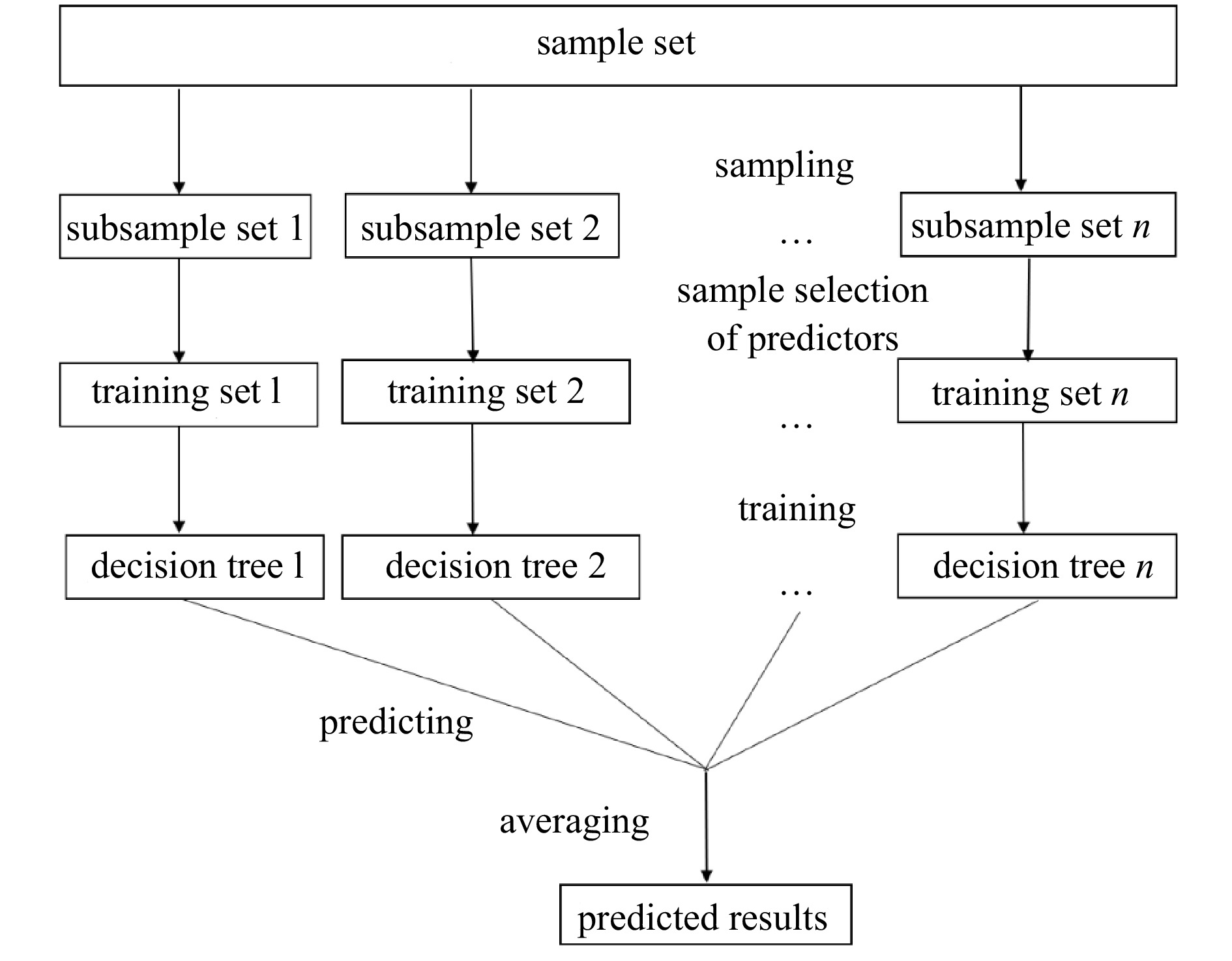
Ali J, Khan R, Ahmad N, et al. 2012. Random forests and decision trees. International Journal of Computer Science Issues, 9(5): 272–278
|
|
Aydoğan B, Ayat B, Öztürk M N, et al. 2010. Current velocity forecasting in straits with artificial neural networks, a case study: Strait of Istanbul. Ocean Engineering, 37(5/6): 443–453, doi: 10.1016/j.oceaneng.2010.01.016
|
|
Barrick D E, Headrick J M, Bogle R W, et al. 1974. Sea backscatter at HF: Interpretation and utilization of the echo. Proceedings of the IEEE, 62(6): 673–680, doi: 10.1109/PROC.1974.9507
|
|
Basañez A, Pérez-Muñuzuri V. 2021. HF radars for wave energy resource assessment offshore NW Spain. Remote Sensing, 13(11): 2070, doi: 10.3390/rs13112070
|
|
Bradbury M C, Conley D C. 2021. Using artificial neural networks for the estimation of subsurface tidal currents from high-frequency radar surface current measurements. Remote Sensing, 13(19): 3896, doi: 10.3390/rs13193896
|
|
Breiman L. 2001. Random forests. Machine Learning, 45(1): 5–32, doi: 10.1023/A:1010933404324
|
|
Chen Yuru, Paduan J D, Cook M S, et al. 2021. Observations of surface currents and tidal variability off of northeastern taiwan from shore-based high frequency radar. Remote Sensing, 13(17): 3438, doi: 10.3390/rs13173438
|
|
Cheng Peng, Valle-Levinson A. 2009. Influence of lateral advection on residual currents in microtidal estuaries. Journal of Physical Oceanography, 39(12): 3177–3190, doi: 10.1175/2009JPO4252.1
|
|
Cosoli S, Pattiaratchi C, Hetzel Y. 2020. High-frequency radar observations of surface circulation features along the south-western Australian coast. Journal of Marine Science and Engineering, 8(2): 97, doi: 10.3390/jmse8020097
|
|
Dinh V N, McKeogh E. 2019. Offshore wind energy: technology opportunities and challenges. In: Proceedings of the 1st Vietnam Symposium on Advances in Offshore Engineering. Singapore: Springer
|
|
Fang Shenguang, Xie Yufeng, Cui Liqin. 2015. Analysis of tidal prism evolution and characteristics of the Lingdingyang Bay at Pearl River estuary. MATEC Web of Conferences, 25: 01006, doi: 10.1051/matecconf/20152501006
|
|
Han Qinghua, Gui Changqing, Xu Jie, et al. 2019. A generalized method to predict the compressive strength of high-performance concrete by improved random forest algorithm. Construction and Building Materials, 226: 734–742, doi: 10.1016/j.conbuildmat.2019.07.315
|
|
Hastie T, Tibshirani R, Friedman J. 2009. Random forests. In: Hastie T, Tibshirani R, Friedman J, eds. The Elements of Statistical Learning. New York: Springer, 587–604
|
|
Immas A, Do N, Alam M R. 2021. Real-time in situ prediction of ocean currents. Ocean Engineering, 228: 108922, doi: 10.1016/j.oceaneng.2021.108922
|
|
Jishun R. 1991. On the geotectonics of southern China. Acta Geologica Sinica-English Edition, 4(2): 111–130, doi: 10.1111/j.1755-6724.1991.mp4002001.x
|
|
Johnston K, Ver Hoef J M, Krivoruchko K, et al. 2001. Using ArcGIS Geostatistical Analyst. Redlands: Esri Redlands
|
|
Kim S J, Kõrgersaar M, Ahmadi N, et al. 2021. The influence of fluid structure interaction modelling on the dynamic response of ships subject to collision and grounding. Marine Structures, 75: 102875, doi: 10.1016/j.marstruc.2020.102875
|
|
Klemas V. 2011. Remote sensing techniques for studying coastal ecosystems: an overview. Journal of Coastal Research, 27(1): 2–17
|
|
Li Ruixiang, Chen Changsheng, Xia Huayong, et al. 2014. Observed wintertime tidal and subtidal currents over the continental shelf in the northern South China Sea. Journal of Geophysical Research: Oceans, 119(8): 5289–5310, doi: 10.1002/2014JC009931
|
|
Li Chuan, Wu Xiongbin, Yue Xianchang, et al. 2017. Extraction of wind direction spreading factor from broad-beam high-frequency surface wave radar data. IEEE Transactions on Geoscience and Remote Sensing, 55(9): 5123–5133, doi: 10.1109/TGRS.2017.2702394
|
|
Lin Mingsen, Xu Dewei, Li Xiaosun. 2003. Application of satellite data in monsoon and circulation of south China sea. In: Proceedings of SPIE 4892, Ocean Remote Sensing and Applications. Hangzhou: SPIE
|
|
Liu Qinyu, Kaneko A, Jilan S. 2008. Recent progress in studies of the South China Sea circulation. Journal of Oceanography, 64(5): 753–762, doi: 10.1007/s10872-008-0063-8
|
|
Liu Zhen, Zhang Zhilong, Zhou Cuiying, et al. 2021. An adaptive inverse-distance weighting interpolation method considering spatial differentiation in 3D geological modeling. Geosciences, 11(2): 51, doi: 10.3390/geosciences11020051
|
|
Ma Lei, Fu Tengyu, Blaschke T, et al. 2017. Evaluation of feature selection methods for object-based land cover mapping of unmanned aerial vehicle imagery using random forest and support vector machine classifiers. ISPRS International Journal of Geo-Information, 6(2): 51, doi: 10.3390/ijgi6020051
|
|
Mantovani C, Corgnati L, Horstmann J, et al. 2020. Best practices on high frequency radar deployment and operation for ocean current measurement. Frontiers in Marine Science, 7: 210, doi: 10.3389/fmars.2020.00210
|
|
Mao Xiaojun, Peng Liuhua, Wang Zhonglei. 2022. Nonparametric feature selection by random forests and deep neural networks. Computational Statistics & Data Analysis, 170: 107436
|
|
Mitchell T M. 1999. Machine learning and data mining. Communications of the ACM, 42(11): 30–36, doi: 10.1145/319382.319388
|
|
Paduan J D, Washburn L. 2013. High-frequency radar observations of ocean surface currents. Annual Review of Marine Science, 5: 115–136, doi: 10.1146/annurev-marine-121211-172315
|
|
Port A, Gurgel K W, Staneva J, et al. 2011. Tidal and wind-driven surface currents in the German Bight: HFR observations versus model simulations. Ocean Dynamics, 61(10): 1567–1585, doi: 10.1007/s10236-011-0412-9
|
|
Ren Lei, Hartnett M. 2017a. Sensitivity analysis of a data assimilation technique for hindcasting and forecasting hydrodynamics of a complex coastal water body. Computers & GeoSciences, 99: 81–90
|
|
Ren Lei, Hartnett M. 2017b. Prediction of surface currents using high frequency CODAR data and decision tree at a marine renewable energy test site. Energy Procedia, 107: 345–350, doi: 10.1016/j.egypro.2016.12.171
|
|
Ren Lei, Hu Zhan, Hartnett M. 2018. Short-term forecasting of coastal surface currents using high frequency radar data and artificial neural networks. Remote Sensing, 10(6): 850, doi: 10.3390/rs10060850
|
|
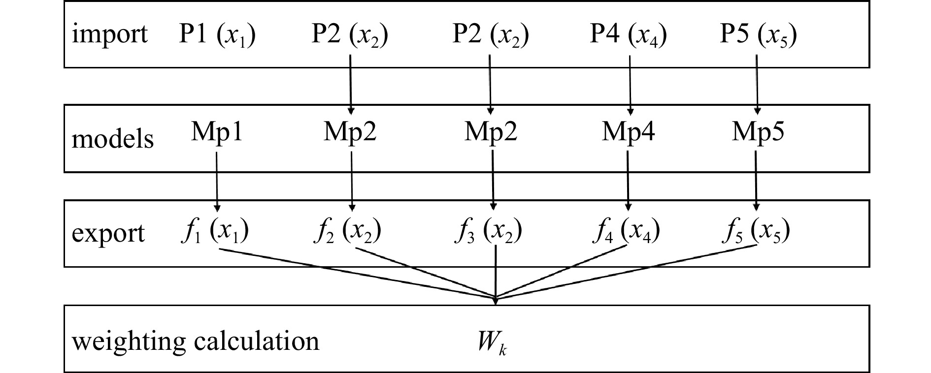
Sagi O, Rokach L. 2018. Ensemble learning: A survey. WIREs: Data Mining and Knowledge Discovery, 8(4): e1249, doi: https://doi.org/10.1002/widm.1249
|
|
Sun Shuo, Zhang Qianli, Sun Junzhong, et al. 2022. Lead–acid battery SOC Prediction using improved adaBoost algorithm. Energies, 15(16): 5842, doi: 10.3390/en15165842
|
|
Vavatsikos A P, Sotiropoulou K F, Tzingizis V. 2022. GIS-assisted suitability analysis combining PROMETHEE II, analytic hierarchy process and inverse distance weighting. Operational Research, 22(5): 5983–6006, doi: 10.1007/s12351-022-00706-0
|
|
Vilibić I, Šepić J, Mihanović H, et al. 2016. Self-organizing maps-based ocean currents forecasting system. Scientific Reports, 6: 22924, doi: 10.1038/srep22924
|
|
Wang Lina, Cao Yu, Deng Xilin, et al. 2023a. Significant wave height forecasts integrating ensemble empirical mode decomposition with sequence-to-sequence model. Acta Oceanologica Sinica, 42(10): 54–66, doi: 10.1007/s13131-023-2246-y
|
|
Wang Yuchen, Imai K, Mulia I E, et al. 2023b. Data Assimilation using high-frequency radar for tsunami early warning: a case study of the 2022 Tonga Volcanic Tsunami. Journal of Geophysical Research: Solid Earth, 128(2): e2022JB025153, doi: 10.1029/2022JB025153
|
|
Wang Wenxiong, Rainbow P S. 2020. Environmental Pollution of the Pearl River Estuary, China. Berlin: Springer
|
|
Wang Shuangling, Zhou Fengxia, Chen Fajin, et al. 2021. Spatiotemporal distribution characteristics of nutrients in the drowned tidal inlet under the influence of tides: a case study of Zhanjiang Bay, China. International Journal of Environmental Research and Public Health, 18(4): 2089, doi: 10.3390/ijerph18042089
|
|
Wei Xing, Cai Shuqun, Zhan Weikang. 2021. Impact of anthropogenic activities on morphological and deposition flux changes in the Pearl River Estuary, China. Scientific Reports, 11(1): 16643, doi: 10.1038/s41598-021-96183-0
|
|
Wen Xuezhi, Shao Ling, Xue Yu, et al. 2015. A rapid learning algorithm for vehicle classification. Information Sciences, 295: 295–406, doi: 10.1016/j.ins.2014.10.040
|
|
Xie Lili, Liu Xia, Yang Qingshu, et al. 2015. Variations of current and sediment transport in Lingding Bay during spring tide in flood season driven by human activities. Journal of Sediment Research (in Chinese), (3): 56–62
|
|
Yang Yun. 2017. Temporal Data Mining via Unsupervised Ensemble Learning. Amsterdam: Elsevier
|
|
Yang Liling, Yang Fang, Yu Shunchao, et al. 2021. The hydrodynamic division of lingdingyang estuary and its application in the impact analysis of large water-related projects. IOP Conference Series: Earth and Environmental Science, 643(1): 012135., doi: 10.1088/1755-1315/643/1/012135
|
|
Ye A L, Robinson I S. 1983. Tidal dynamics in the South China Sea. Geophysical Journal International, 72(3): 691–707, doi: 10.1111/j.1365-246X.1983.tb02827.x
|
|
Yin Xunqiang, Shi Junqiang, Qiao Fangli. 2018. Evaluation on surface current observing network of high frequency ground wave radars in the Gulf of Thailand. Ocean Dynamics, 68(4): 575–587
|

Figures(11) / Tables(7)

Supported by:
Beijing Renhe Information Technology Co. Ltd

Bingxin Huang, Yue Chu, Rongjuan Wang, Yixiao Wang, Lanping Ding. Effects of main ecological factors on the growth of marine green alga Caulerpa sertularioides using the response surface methodology[J]. Acta Oceanologica Sinica, 2023, 42(11): 90-97. doi: 10.1007/s13131-023-2171-0

| Factor | Irradiance /(μmol·m−2·s−1) | Temperature/℃ | Salinity |
| Low | 31.25 | 22 | 25 |
| High | 43.75 | 28 | 35 |
DownLoad:
CSV
| Serial number | Irradiance/ (μmol·m−2·s−1) | Temperature/℃ | Salinity | SGR/% |
| 1 | 37.5 | 22 | 35 | 2.84 |
| 2 | 37.5 | 25 | 30 | 4.62 |
| 3 | 37.5 | 28 | 35 | 3.06 |
| 4 | 37.5 | 25 | 30 | 4.52 |
| 5 | 37.5 | 22 | 25 | 2.46 |
| 6 | 43.75 | 28 | 30 | 3.25 |
| 7 | 31.25 | 22 | 30 | 1.93 |
| 8 | 37.5 | 25 | 30 | 4.52 |
| 9 | 43.75 | 22 | 30 | 3.20 |
| 10 | 31.25 | 28 | 30 | 2.65 |
| 11 | 43.75 | 25 | 25 | 3.41 |
| 12 | 37.5 | 25 | 30 | 4.70 |
| 13 | 31.25 | 25 | 35 | 2.63 |
| 14 | 37.5 | 28 | 25 | 3.26 |
| 15 | 31.25 | 25 | 25 | 2.38 |
| 16 | 43.75 | 25 | 35 | 3.38 |
| 17 | 37.5 | 25 | 30 | 4.62 |
DownLoad:
CSV
| Source | Sum of squares | df | Mean square | F value | P value | Significance |
| Model | 12.89 | 9 | 1.43 | 304.92 | <0.000 1 | Significant |
| A−irradiance | 1.67 | 1 | 1.67 | 355.29 | <0.000 1 | − |
| B−temperature | 0.4 | 1 | 0.4 | 85.16 | <0.000 1 | − |
| C−salinity | 0.02 | 1 | 0.019 | 4.08 | 0.083 | − |
| AB | 0.11 | 1 | 0.11 | 23.76 | 0.001 8 | − |
| AC | 0.02 | 1 | 0.022 | 4.64 | 0.068 | − |
| BC | 0.08 | 1 | 0.083 | 17.67 | 0.004 | |
| A2 | 3.4 | 1 | 3.4 | 724.44 | <0.000 1 | − |
| B2 | 3.74 | 1 | 3.74 | 796.58 | <0.000 1 | − |
| C2 | 2.34 | 1 | 2.34 | 498.31 | <0.000 1 | − |
| Residual | 0.033 | 7 | 4.70 × 10⁻³ | − | − | − |
| Lack of fit | 9.07 × 10⁻³ | 3 | 3.02 × 10⁻³ | 0.51 | 0.80 | Insignificant |
| Pure error | 0.024 | 4 | 5.95 × 10⁻³ | − | − | − |
| Cor total | 12.93 | 16 | − | − | − | − |
| Note: df: Degrees of Freedom. Cor total: This row shows the amount of variation around the mean of the observations. The model explains part of it, the residual explains the rest. | ||||||
DownLoad:
CSV
| Factor | Irradiance /(μmol·m−2·s−1) | Temperature/℃ | Salinity |
| Low | 31.25 | 22 | 25 |
| High | 43.75 | 28 | 35 |
| Serial number | Irradiance/ (μmol·m−2·s−1) | Temperature/℃ | Salinity | SGR/% |
| 1 | 37.5 | 22 | 35 | 2.84 |
| 2 | 37.5 | 25 | 30 | 4.62 |
| 3 | 37.5 | 28 | 35 | 3.06 |
| 4 | 37.5 | 25 | 30 | 4.52 |
| 5 | 37.5 | 22 | 25 | 2.46 |
| 6 | 43.75 | 28 | 30 | 3.25 |
| 7 | 31.25 | 22 | 30 | 1.93 |
| 8 | 37.5 | 25 | 30 | 4.52 |
| 9 | 43.75 | 22 | 30 | 3.20 |
| 10 | 31.25 | 28 | 30 | 2.65 |
| 11 | 43.75 | 25 | 25 | 3.41 |
| 12 | 37.5 | 25 | 30 | 4.70 |
| 13 | 31.25 | 25 | 35 | 2.63 |
| 14 | 37.5 | 28 | 25 | 3.26 |
| 15 | 31.25 | 25 | 25 | 2.38 |
| 16 | 43.75 | 25 | 35 | 3.38 |
| 17 | 37.5 | 25 | 30 | 4.62 |
| Source | Sum of squares | df | Mean square | F value | P value | Significance |
| Model | 12.89 | 9 | 1.43 | 304.92 | <0.000 1 | Significant |
| A−irradiance | 1.67 | 1 | 1.67 | 355.29 | <0.000 1 | − |
| B−temperature | 0.4 | 1 | 0.4 | 85.16 | <0.000 1 | − |
| C−salinity | 0.02 | 1 | 0.019 | 4.08 | 0.083 | − |
| AB | 0.11 | 1 | 0.11 | 23.76 | 0.001 8 | − |
| AC | 0.02 | 1 | 0.022 | 4.64 | 0.068 | − |
| BC | 0.08 | 1 | 0.083 | 17.67 | 0.004 | |
| A2 | 3.4 | 1 | 3.4 | 724.44 | <0.000 1 | − |
| B2 | 3.74 | 1 | 3.74 | 796.58 | <0.000 1 | − |
| C2 | 2.34 | 1 | 2.34 | 498.31 | <0.000 1 | − |
| Residual | 0.033 | 7 | 4.70 × 10⁻³ | − | − | − |
| Lack of fit | 9.07 × 10⁻³ | 3 | 3.02 × 10⁻³ | 0.51 | 0.80 | Insignificant |
| Pure error | 0.024 | 4 | 5.95 × 10⁻³ | − | − | − |
| Cor total | 12.93 | 16 | − | − | − | − |
| Note: df: Degrees of Freedom. Cor total: This row shows the amount of variation around the mean of the observations. The model explains part of it, the residual explains the rest. | ||||||
 DownLoad: