Yuxin Shi, Hailong Liu, Xidong Wang, Quanan Zheng. Responses of the Southern Ocean mixed layer depth to the Eastern and Central Pacific El Niño events during austral winter[J]. Acta Oceanologica Sinica.
Citation:
Yuxin Shi, Hailong Liu, Xidong Wang, Quanan Zheng. Responses of the Southern Ocean mixed layer depth to the Eastern and Central Pacific El Niño events during austral winter[J]. Acta Oceanologica Sinica.
Yuxin Shi, Hailong Liu, Xidong Wang, Quanan Zheng. Responses of the Southern Ocean mixed layer depth to the Eastern and Central Pacific El Niño events during austral winter[J]. Acta Oceanologica Sinica.
Citation:
Yuxin Shi, Hailong Liu, Xidong Wang, Quanan Zheng. Responses of the Southern Ocean mixed layer depth to the Eastern and Central Pacific El Niño events during austral winter[J]. Acta Oceanologica Sinica.
School of Oceanography, Shanghai Jiao Tong University, Shanghai 200240, China
2.
College of Oceanography, Hohai University, Nanjing 210098, China
3.
Department of Atmospheric and Oceanic Science, University of Maryland at College Park, College Park 20742, USA
Funds:
Oceanic Interdisciplinary Program of Shanghai Jiao Tong University (project number SL2021ZD204); Sino-German Mobility Program (Grant no. M0333); Shanghai Frontiers Science Center of Polar Science (SCOPS).
Based on the Ocean Reanalysis System version 5 (ORAS5) and the fifth-generation reanalysis datasets (ERA5) derived from Medium-Range Weather Forecasts (ECMWF), we investigate the different impacts of the Central Pacific (CP) El Niño and the Eastern Pacific (EP) El Niño on the Southern Ocean (SO) mixed layer depth (MLD) during austral winter. The MLD response to the EP El Niño shows a dipole pattern in the South Pacific, namely the MLD dipole, which is the leading El Niño-induced MLD variability in the SO. The tropical Pacific warm sea surface temperature anomaly (SSTA) signal associated with the EP El Niño excites a Rossby wave train propagating southeastward and then enhances the Amundsen Sea Low (ASL). This results in an anomalous cyclone over the Amundsen Sea. As a result, the anomalous southerly wind to the west of this anomalous cyclone advects colder and drier air into the southeast of New Zealand, leading to surface cooling through less total surface heat flux, especially surface sensible heat (SH) flux and latent heat (LH) flux, and thus contributing to the ML deepening. The east of the anomalous cyclone brings warmer and wetter air to the southwest of Chile, but the total heat flux anomaly shows no significant change. The warm air promotes the sea ice melting and maintains fresh water, which strengthens stratification. This results in a shallower MLD. During the CP El Niño, the response of MLD shows a separate negative MLD anomaly center in the central South Pacific. The Rossby wave train triggered by the warm SSTA in the central Pacific Ocean spreads to the Amundsen Sea, which weakens the ASL. Therefore, the anomalous anticyclone dominates the Amundsen Sea. Consequently, the anomalous northerly wind to the west of anomalous anticyclone advects warmer and wetter air into the central and southern Pacific, causing surface warming through increased SH, LH and longwave (LW) radiation flux, and thus contributing to the ML shoaling. However, to the east of the anomalous anticyclone, there is no statistically significant impact on the MLD.
Figure 1. Time series of (a) Niño 3 index (blue line) from NOAA and Nep index (red line) based on Eq. (2), and (b) Niño 4 index (blue line) from NOAA and Ncp index (red line) based on Eq. (2). Grey dashed lines denote one standard deviation of Nep and Ncp indices. Cor indicates correlations between two curves in each panel.
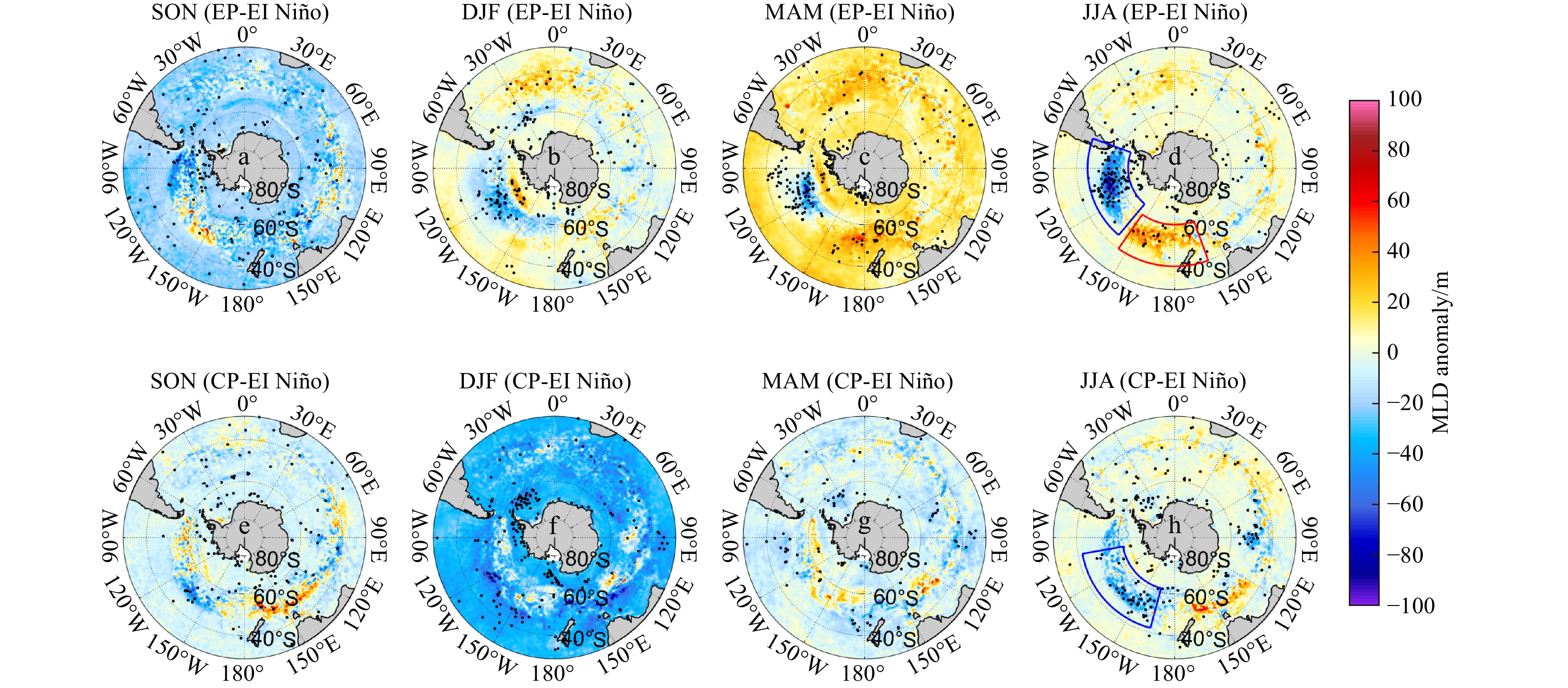
Figure 2. Composite images of MLD (unit: m) anomaly derived from the ORAS5 in austral (a), (e) spring (SON), (b), (f) summer (DJF), (c), (g) autumn (MAM), and (d), (h) winter (JJA) for (a)–(d) EP El Niño and (e)–(h) CP El Niño events. The black stippled areas represent that the results are statistically significant at the 95% confidence level. Box 1 (40°–60°S, 160°E–145°W) and Box 2 (45°–65°S, 140°–70°W) in (d) and the Box 3 (42°–62°S, 165°–100°W) in (h) indicate the focus areas
Figure 3. Composite images of SSTA (unit: °C) observed from the ERA5 for EP (a) and CP (b) El Niño events in austral winter (JJA). The black stippled areas represent that the results are statistically significant at the 95% confidence level. Red and blue boxes are the same as in Figs 2d and h.
Figure 4. Composite images of (a) and (b) 300 hPa, (c) and (d) 700 hPa, and (e) and (f) 850 hPa geopotential height (unit: m) anomaly derived from the ERA5 for (a), (c) and (e) EP El Niño and (b), (d) and (f) CP El Niño events. The gray shadings represent the results statistically significant at the 95% confidence level. Red and blue boxes are the same as in Figs 2d and h.
Figure 5. Composite images of 300 hPa (a) and (b) zonal wind anomaly (unit: m/s), and (c) and (d) PV (unit: m2·K/(kg·s)) anomaly derived from the ERA5 for (a) and (c) EP El Niño and (b) and (d) CP El Niño events. The black stippled areas represent the results statistically significant at the 95% confidence level. Red and blue boxes are the same as in Figs. 2d and h.
Figure 6. Composite images of a and b SLP anomaly (unit: hPa), and c and d anomalous 10 m wind (vectors) as well as wind speed (color) anomaly (unit: m/s) derived from the ERA5 for a and c EP El Niño and b and d CP El Niño events. The gray shadings and black stippled areas represent the results statistically significant at the 95% confidence level. Red and blue boxes are the same as in Figs 2d and h.
Figure 7. Composite images of a and b air temperature anomaly at 2 m (unit: °C), and c and d 1000 hPa specific humidity anomaly (unit: g/kg) derived from the ERA5 for a, c EP El Niño and b, d CP El Niño events. The black stippled areas represent the results statistically significant at the 95% confidence level. Red and blue boxes are the same as in Figs 2d and h.
Figure 8. Composite images of surface SH anomaly (a and b), LH anomaly (c and d), net LW anomaly (e and f), net SW anomaly (g and h), and total surface heat flux anomaly (i and j) (unit: W/m2) derived from the ERA5 for a, c, e, g, and i EP El Niño and b, d, f, h, and j CP El Niño events. The positive anomaly represents downward. The black stippled areas represent the results statistically significant at the 95% confidence level. Red and blue boxes are the same as in Figs 2d and h.
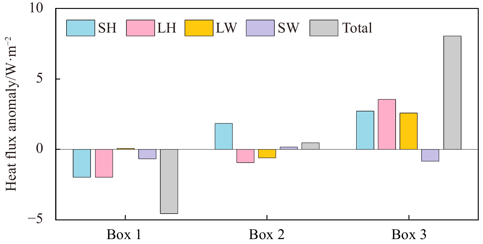
Figure 9. Contributions of net heat flux components (unit: W/m2) to the MLD anomaly during EP and CP El Niño events. The contributions are calculated from averaged anomaly over Box 1 and Box 2 in Figs. 8a, c, e, g and i for EP El Niño events, and Box 3 in Figs 8b, d, f, h and j for CP El Niño events.
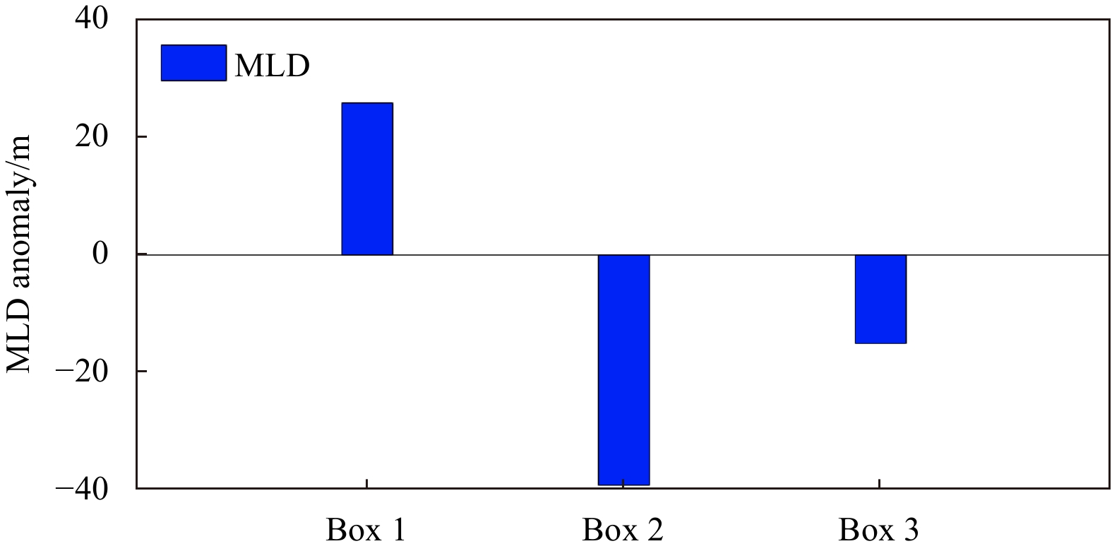
Figure 10. Magnitudes of MLD variation (unit: m) derived from the ORAS5 during the EP and CP El Niño events. The magnitudes are estimated by averaging anomaly over the red and blue boxes in Fig. 2d and the blue box in Fig. 2h.
Figure 11. Composite pictures of SIC anomaly derived from the ORAS5 during (a) EP El Niño events, and (b) CP El Niño events. The black stippled areas represent the results statistically significant at the 95% confidence level. Red and blue boxes are the same as in Figs. 2d and h.
Figure 12. Schematic diagram illustrating the differences of critical elements during EP and CP El Niño events. Red and blue boxes are the same as in Figs. 2d and h.


 DownLoad: