

Figure
1.
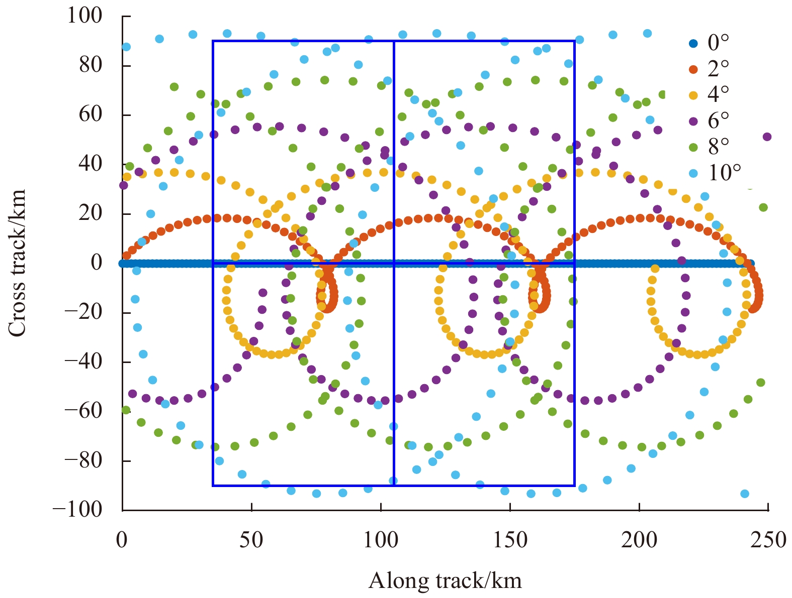
Horizontal sampling of wave investigation and monitoring data (Tison et al., 2019).
| Citation: | Jingwei Gu, Xiuzhong Li, Yijun He. A speckle noise suppression method based on surface waves investigation and monitoring data[J]. Acta Oceanologica Sinica, 2023, 42(1): 131-141. doi: 10.1007/s13131-022-2103-4

|
Ocean waves are a volatile phenomenon that often occurs in the ocean, which includes wind waves, swell waves, and near-shore waves. An ocean wave is composed of an infinite number of constituent waves of different amplitudes, frequencies, directions, and phases. A wave spectrum is a map that describes the distribution of wave frequency and direction relative to the internal energy. It is an important statistical property of random sea waves. It not only contains second-order information of ocean waves but also shows their external form and internal characteristics. Therefore, studying wave spectra are important for understanding wave characteristics and forecasts. It is critical in fields such as air-sea interaction, upper ocean dynamics, wave prediction, ocean remote sensing, ocean engineering, and so on.
Wave measurement methods mainly include direct measurement and remote sensing. Direct measurement methods are classified into two: fixed point measurement and array methods. The direct measurement method can measure the wave more accurately, but it has disadvantages such as narrow measurement range, discontinuous time, and is highly affected by the environment. Therefore, measuring the space-time continuous-wave direction spectra using the direct measurement method is difficult. Therefore, remote sensing technology must be used for measurement. There are two main remote sensing methods: marine radar and synthetic aperture radar (SAR) methods. The marine radar method cannot be used for all-weather global measurement, and the measurement results contain much noise; whereas, the SAR method cannot be used for a long time. Surface waves investigation and monitoring (SWIM) is a new measuring instrument proposed to solve these problems. In spite of this, SAR still plays an irreplaceable role in some fields. And there have been some meaningful research about SAR ocean wave observations. These researches provide methods to calculate the significant wave height of waves by SAR (Wang et al., 2018, 2022; Quach et al., 2021).
SWIM is a scanning beam true aperture radar that was proposed in the 1980s (Jackson et al., 1985a, b). The main principle of SWIM is that the normalized radar cross-section is sensitive to the local tilt of the sea surface at a small incident angle, but it is almost insensitive to the small-scale wind roughness effect and hydrodynamic modulation, which is caused by the interaction between long and short waves. In subsequent research, several airborne platforms were equipped with SWIM (Hauser et al., 1992; Vandemark et al., 1994; Caudal et al., 2014). The SWIM is being used for the first time on a space-borne platform with the Chinese-French Oceanography Satellite (CFOSAT).
CFOSAT was launched in October 2018 after being developed jointly by China and France. The SWIM on CFOSAT is a real-aperture radar in the Ku-band (13.6 GHz) that illuminates the surface sequentially with six incidence angles (0°, 2°, 4°, 6°, 8°, and 10°) and an antenna aperture of approximately 2°. The 0° beam is a finite pulse beam with an incidence angle of 0°, which is used to measure a significant wave height (SWH) and wind speed (WS). The other beams are five pen-shaped beams with a central axis deviating from the 0° beam direction by 2°, 4°, 6°, 8°, and 10°. The two-dimensional (2D) ocean-wave spectra are obtained by rotating an antenna at a speed of 5.6 revolutions per minute (Tison et al., 2009, 2019; Hauser et al., 2010; Dong et al., 2011).
Because it is the first time, SWIM has been used on a space-borne platform, some problems remain, such as large speckle noise in the 2D directional wave spectra product (Hauser et al., 2021). In the measurement of wave spectrum and speckle, noise is unavoidable and speckle noise is a common phenomenon in all coherent imaging systems. When a radar detects the sea surface, the roughness of the sea surface results in many independent scattering surface elements in a resolution unit, and the radar antenna can receive the echo signal of each scattering surface element. Meanwhile, each signal is in a coherent superposition. Because the distance between each scattering surface element and radar is different, the phase of each echo differs. A strong signal is generated when the echo phase is consistent, and a weak signal is generated when the echo phase is inconsistent. This phenomenon results in a patchwork of light and dark spots on the image, which is known as the speckle noise. This is caused by a random interference phenomenon that affects the radar observation, and the scale is equivalent to the wavelength of the incident radar wave (Singh and Shree, 2016). Therefore, speckle noise exists in the 2D directional wave spectra measured by SWIM. When the fluctuation spectrum is estimated using independent samples, the noise spectral density can be expressed as a function of independent samples (Hauser et al., 2001). The number of independent samples in the along-track direction (that is, within 15° of the satellite’s orbit) of SWIM decreases sharply because of the decrease in Doppler bandwidth, which leads to a significant increase in the noise spectral density, resulting in speckle noise in the along-track direction was significantly greater than that in other directions of SWIM (Hauser et al., 2021).
Many studies on speckle noise have been conducted using SAR. In the 1980s, Lee et al. proposed a spatial local filtering method, which uses a sigma filter to smooth the speckled image (Lee, 1980, 1981a, b, 1983). Subsequently, many denoising methods, such as transform domain filtering, adaptive morphological filtering, and wavelet transform methods were proposed (Argenti and Alparone, 2002; Yu and Acton, 2002; Deledalle et al., 2009, 2015; Ahmed et al., 2010; Raju et al., 2013; Yamazaki et al., 2017). In addition to these methods, the neural network method, which has recently gained popularity, has many applications in the field of speckle-noise suppression (Owirka et al., 1999; Achim et al., 2003; Patnaik and Casasent, 2005; Morgan, 2015; Chen et al., 2016; Chierchia et al., 2017; Kwak et al., 2019; Mohan et al., 2021).
Although SWIM and SAR are radars with similar noise generation mechanisms, they differ in speckle noise suppression. As a new multi-beam real-aperture radar, the study of speckle noise suppression on SWIM is not as extensive as that on SAR. In 2020, Hauser et al. (2021) proposed an empirical method for suppressing speckle noise from 2D directional wave spectra of SWIM. This method is mainly based on the empirical formula of speckle noise established by numerous data to achieve noise suppression, which has been applied to the SWIM V5.1.2 data. However, this method can still be improved in some ways. For example, this method denoises excessively in the along-track direction, which leads to some missing values in the 2D directional wave spectra in some cases. Additionally, this method can be improved to deal with abnormal noise, which results in some abnormally large values in the 2D directional wave spectra.
To solve these problems, this study proposes a new speckle noise suppression method based on SWIM data that use rational transfer function filtering (RTFF) and noise ratio (NR) control. This method was called the spectral classification-threshold control (SCTC) method. The structure of this study is as follows: the second section introduces the data used in this study; the third section introduces the SCTC method. In fourth section, the results of the SCTC method are compared with the SWIM data, WaveWatch III (WW3) data and National Data Buoy Center (NDBC) buoy in situ observations data. The fifth section is the conclusion of this study.
In this study, SWIM-level 1b (L1b) and level 2 (L2) products for version 5.1.2 are used. The period of data is from May 1, 2019, to April 30, 2020. The data is selected from the first four days of each month. In June 2019, the data for 5–8 days are selected because of the lack of data from the 1st to 4th day. The data selected in this way is to eliminate seasonal and spatial variations in wave spectra, allowing these data to be represented in all directions and locations. The entire year wave data were not selected to reduce the amount of calculation, and the interval selection like this met our needs.
The acquisition of L1b only uses a beam of 6°, 8°, and 10°, and its role is to generate a modulation spectrum. The role of the L2 processing step is to generate geophysical data products that reconstruct 2D observations. The data of L1b are stored according to macrocycle, and variables such as fluctuation spectra, azimuth, and latitude are used. The L2 defines product units that covers both sides of the satellite’s orbit, and it corresponds to an area of approximately 70 km×90 km (Fig. 1). In Fig. 1, each blue box is a product unit named box, scattered points of different colors represent the scanning track of different beams, the horizontal coordinate represents the distance in the running direction of the satellite, and the vertical coordinate represents the distance perpendicular to the running direction of the satellite. The data of L2 contain several physical parameters, such as SWH and WS, which are divided into 24 azimuths, each azimuth is 15°.
To verify the effect of the SCTC method, data of WW3 are used as referenced data. The resolution in time is 3 h and that in space is 0.5°×0.5° of referenced data we used. WW3 is the third generation wave model developed by the National Oceanic and Atmospheric Administration (NOAA) and the National Centers for Environmental Prediction (NCEP) based on the Whac-a-mole model. It is a development of WaveWatch and WaveWatch 2. WW3 has been improved in many important aspects, such as governing equations, the model structure, numerical methods, and physical parameterization. WW3 is commonly used in wave climate analysis (Gallagher et al., 2016), and it has been demonstrated to be capable of simulating waves in key areas such as the Pacific and adjacent sea areas of China (Gallagher et al., 2014; Zheng et al., 2016, 2018; Bi et al., 2015; Guo et al., 2015; He and Xu, 2016; Shukla and Kinter, 2016). Furthermore, WW3 can be used to study the typhoon waves (Shao et al., 2018; Sheng et al., 2019), and it provides an exchange of wave-current interactions, indicating that it considers the influence of ocean currents. In this study, the data of WW3 from 2019 to 2020 were obtained from the NCEP NOAA Operational Model Archive and Distribution System, Global Data Service, and Distributed Oceanographic Data Systems data servers. The window with a time threshold of 10 min and a space threshold of 10 km was selected to match WW3 data with the SWIM data mentioned above. The matched data are deemed observations of the same wave spectrum.
The NDBC buoy in situ observations data we used are obtained from NDBC Stations 44005, 44025 and 46100. The Stations 44005 and 44025 are owned and maintained by National Data Buoy Center while the Station 46100 is owned and maintained by Ocean Observatories Initiative. Station 44005’s latitude is 43.201°N and its longitude is 69.127°W. The air temp height is 4.4 m above site elevation, the anemometer height is 4.9 m above site elevation, the barometer elevation is 0.3 m above mean sea level and the sea temp depth is 0.6 m below water line of Station 44005. Station 44025’s latitude is 40.251°N and its longitude is 73.164°W. The air temp height is 3.7 m above site elevation, the anemometer height is 4.1 m above site elevation, the barometer elevation is 2.7 m above mean sea level and the sea temp depth is 1.5 m below water line of Station 44025. Station 46100’s latitude is 46.851°N and its longitude is 124.972°W. The air temp height is 4 m above site elevation, the anemometer height is 4.5 m above site elevation, the barometer elevation is 3.95 m above mean sea level and the sea temp depth is 1.15 m below water line of Station 46100. We use variable named “WVHT” as SWH, “DPD” as the dominant wave period and “MWD” as the dominant wave direction (DWAD) of standard meteorological data of these stations. To make comparison easier, we turn the dominant wave period to the dominant wavelength (DWAL) by dispersion relationship.
This section discusses the SCTC method. There are two types of noise in fluctuation spectra, which are background speckle noise and speckle noise caused by Doppler bandwidth reduction (SNDBR). The calculation and suppression methods of these noises are discussed sequentially.
In addition to wave information, fluctuation spectra in the data of L1b of SWIM contain noise, which must be suppressed during inversion (Jackson et al., 1985a, b; Hauser et al., 2017). The expression of noise is shown in Eq. (1):
| $$ {P}_{\mathrm{d}{\mathrm{s}}_{0}}\left(k\right)\approx {\text{δ}} \left(k\right)+{P}_{\text{IR}}\left(k\right)\times {P}_{\mathrm{m}}\left(k\right)+{P}_{\text{sp}}\left(k\right) ,$$ | (1) |
where
| $$ {P}_{\text{sp}}\left(k\right)=\frac{1}{{N}_{\text{ind}}}\frac{{{\text{δ}}}r}{2\text{π}}\frac{1}{\rm{sin}\;\theta \times {\rm{tri}}\left(\dfrac{k}{2\text{π}}\dfrac{{{\text{δ}}}r}{\rm{sin}\;\theta }\right)}, $$ | (2) |
where tri is the trigonometric function,
| $$ {P}_{\mathrm{s}}\left(k\right)=\frac{1}{{N}_{\text{ind}}\sqrt{2\mathrm{\pi }}}\frac{\Delta x}{2\sqrt{2\;{{\rm{ln}}}\;2}}, $$ | (3) |
where
| Variable | Beam 0° | Beam 2° | Beam 4° | Beam 6° | Beam 8° | Beam 10° |
| Time duration/ms | 55.4 | 22.6 | 22.6 | 34.4 | 40.5 | 44.2 |
| Number of integrated echoes | 264 | 97 | 97 | 156 | 186 | 204 |
| Number of averaged range bins | 1 | 4 | 4 | 2 | 3 | 3 |
 DownLoad:
CSV
DownLoad:
CSV
However, because of other factors, this setting of
According to Hauser et al. (2021), in the non-orbital direction, speckle noise is affected only by radar parameters, and it has nothing to do with sea state and latitude. Meanwhile, in the along-track direction, this type of speckle noise exists in addition to SNDBR. Therefore, we refer to this type of speckle noise as background speckle noise. The impact of wave information must be minimized to suppress this noise. Because the direction of the fluctuation spectrum with the smallest variance in every 180° azimuth is the direction containing the least wave information (Hauser et al., 2021), the fluctuation spectrum in this direction is used as the background speckle noise (Fig. 2).

The background speckle noise agrees well with the theoretical formula (Eq. (2)), thus the empirical formula of background speckle noise can be established.
In the along-track direction, there is SNDBR besides the background speckle noise mentioned in the previous section. The noise should be classified according to its influencing factors to obtain the empirical formula of SNDBR.
Generally, three factors can affect SNDBR: latitude, sea surface condition, and the beams of SWIM (Hauser et al., 2021). Additionally, sea surface conditions can be expressed by SWH and WS. Therefore, four variables, such as latitude, SWH, WS, and beam, are selected to classify SNDBR.
The above-mentioned data of L2 are used for classification. The classification of 14 categories for latitude from 70°N to 70°S is set up, and the interval is 10°. The classification of three categories for sea surface condition is also set up (WS<5 m/s and SWH<2 m,
According to the classification above, SNDBR in the fluctuation spectra of one class is the same. Therefore, if the SNDBR of one fluctuation spectrum is obtained, the SNDBR of other fluctuation spectra in the same class can also be obtained. To obtain the SNDBR of each class, the real wave information in the along-track is must be obtained first. Therefore, fluctuation spectra are averaged based on classification. The average of 19 categories among 126 classifications is shown in Fig. 3. Because the selected data cover one year, and the fluctuation spectra belonging to the same class have similar elements such as sea surface conditions and geographical information, the real wave information contained in each of the 126 fluctuation spectra should be distributed almost uniformly in all directions.

According to the above research, background speckle noise exists in all directions of the 126 fluctuation spectra. The obtained empirical formula of background speckle noise is used to calculate background speckle noise and suppress the background speckle noise from the above-mentioned averaged fluctuation spectra acquired. Thus, 126 new fluctuation spectra without background speckle noise are obtained. Only SNDBR exists in these new fluctuation spectra. Therefore, in the non-orbital direction, these new fluctuation spectra only contain real wave information. The real wave information is almost uniform in all directions, as previously mentioned. Therefore, the real wave information of each class is obtained.
However, there are errors in the measurement, which can affect the average of the fluctuation spectrum, and the samples are not infinity. Therefore, the ideal situation is difficult to achieve and the real wave information may have a small difference between each direction. This can cause some errors in the estimation of real wave information and the error can be intensified in the presence of the fluctuation spectrum with significant abnormal noise. To obtain the real wave information from the along-track more accurately, RTFF expressed in Eq. (4) is used to filter each wavenumber of each fluctuation spectrum.
| $$ Y\left(z\right)=\frac{b\left(1\right)+b\left(2\right){z}^{-1}+\dots +b\left({n}_{b}+1\right){z}^{-{n}_{b}}}{1+a\left(2\right){z}^{-1}+\dots +a\left({n}_{a}+1\right){z}^{-{n}_{a}}}X\left(z\right), $$ | (4) |
where X(z) represents the input fluctuation spectrum, Y(z) represents the filtered fluctuation spectrum, z is the transform domain.

According to the real wave information obtained above, an SNDBR of 126 classifications can be obtained. The fluctuation spectrum samples selected are evenly distributed over one year and are classified based on the characteristics of the influence of SNDBR. Therefore, among the 126 classifications divided, SNDBR belonging to the same category accounts for the same proportion in the corresponding fluctuation spectra. The proportion of SNDBR and fluctuation spectrum is used as the NR threshold of each class.
During denoising, after SNDBR is calculated, the NR of SNDBR is must also be calculated. If the NR calculated is less than the corresponding NR threshold, the noise corresponding to the NR threshold is used as SNDBR at this position.
We selected fluctuation spectra of one orbit on June 6, 2019, to obtain the denoised 2D directional wave spectra using the SCTC method. The denoised 2D directional wave spectrum of the 220th left box of this orbit is shown in Fig. 5.

Figure 6 shows the same 2D directional wave spectrum as Fig. 5, but it is not denoised.

Figure 6 shows SNDBR, which can affect DWAL and DWAD. SNDBR is significantly large and covers all real wave information. SNDBR is significantly suppressed after the SCTC method is used (Fig. 5). DWAL and DWAD are then successfully calculated.
In order to compare the denoising effects of SCTC method with other methods, we select one case to calculate the denoising results of SCTC method and compare them with SWIM products and WW3 products. We also select NDBC buoys to validate the denoising effects of SCTC method.
The 2D directional wave spectra provided in the SWIM version 5.1.2 are generated by fluctuation spectra, which are dealt with using the empirical denoising method proposed by Hauser et al. (2021). The 2D directional wave spectrum of SWIM products, which has the same time and location as the above-mentioned SCTC method product, is selected. It is shown in Fig. 7.

There are two obvious areas for improvement in SWIM products. (1) There are small white pixels at 0°–15° azimuth and 180°–195° azimuth in Fig. 7. These small white blocks are due to an overestimation of noise, which causes the real wave information to be treated as noise and suppressed. This leads to partial wave information loss. (2) The 2D directional wave spectrum at the azimuth angles of 15°–30° and 195°–210° in Fig. 7 still retains noise. This means that some large abnormal noises are not suppressed.
Both of these two factors can be attributed to the denoising method used in SWIM products. According to Hauser et al. (2021), quadratic polynomial fitting to fluctuation spectra is used in SWIM products to calculate SNDBR. Generally, scatters are uniformly distributed near the fitting curve, which causes SNDBR of scatters smaller than the fitting curve to be larger than fluctuation spectra, resulting in the above-mentioned excessive along-track denoising .
In addition to causing excessive along-track denoising, the quadratic polynomial fitting lacks representativeness for some fluctuation spectra with abnormally large noise. Therefore, when these fluctuation spectra are denoised, several noises will be left, which will cover the real wave information.
In these cases, the SCTC method makes some improvements. First, the SCTC method uses fluctuation spectra within a year and a global space span to increase representativeness. Second, the real wave information is isotropic after averaging over a large time-space window. According to these properties, the SCTC method calculates real wave information to obtain SNDBR. This can reduce the error compared with quadratic polynomial fitting. Third, in the SCTC method, NR control is proposed. This can affect the suppression of abnormally large noise.
Because WW3 products are selected as reference data, the SCTC method and SWIM products are compared with them. WW3 products are time and space matched with the SCTC method and SWIM products for consistency comparison. The 2D directional wave spectrum of WW3 products matched with that of Fig. 5 is shown in Fig. 8.

According to Fig. 8, the SWH of the 2D directional wave spectrum of WW3 products is 4.2 m, DWAL of that is 89 m, and DWAD of that is 176°. In comparison, the SWHs of SCTC method and SWIM products are 3.8 m and 3.7 m, respectively, DWALs of that of SCTC method and SWIM products are both 151 m, and DWADs of SCTC method and SWIM products are 162° and 131°, respectively. In the case of SWH, the SWH error ratio equations of the SCTC method and SWIM products are as follows:
| $$ an{o}_{\text{SCTC}}=\frac{\mathrm{abs}\left({\rm{SWH}}_{\text{SCTC}}-{\rm{SWH}}_{\text{WW3}}\right)}{{\rm{SWH}}_{\text{WW3}}} ,$$ | (5) |
| $$ an{o}_{\text{SWIM}}=\frac{\mathrm{abs}\left({\rm{SWH}}_{\text{SWIM}}-{\rm{SWH}}_{\text{WW3}}\right)}{{\rm{SWH}}_{\text{WW3}}}, $$ | (6) |
where
The comparison above is based on WW3 data as reference data. As we all know, the buoy in situ measurements data are also important. However, the scarcity of buoy observation makes it difficult to be used in comparison between large quantities of data. Here, we choose two cases of NDBC Buoy 46100 to compare with SCTC method, so as to verify the denoising effects of SCTC method. The comparison results are shown in Tables 2 and 3. The time of NDBC data in Table 2 is 3:10 UTC on November 26, 2019, while the time of SWIM products and SCTC method results is 2:56:33 UTC on November 26, 2019. The time of NDBC data in Table 3 is 3:10 UTC on December 9, 2019, while the time of SWIM products and SCTC method results is 2:56:30 UTC on December 9, 2019. ano is used to show errors of SWIM and SCTC products. Take SWH for example, the equation of
| SWH/m | $ {ano}_{{\rm{SWH}}} $ | DWAL/m | $ {ano}_{\mathrm{DWAL}} $ | DWAD/(°) | $ {ano}_{\mathrm{DWAD}} $ | |
| Buoy | 3.62 | − | 275.90 | − | 110.00 | − |
| SWIM products | 3.89 | 7.46% | 164.91 | 40.23% | 114.37 | 3.97% |
| SCTC results | 3.85 | 6.35% | 268.07 | 2.84% | 108.54 | 1.33% |
| Note: SWIM: surface waves investigation and monitoring; SCTC: spectral classification-threshold control; SWH: significant wave height; DWAL: dominant wavelength: DWAD: dominant wave direction. − represents no data. | ||||||
DownLoad:
CSV
| SWH/m | $ {ano}_{{\rm{SWH}}} $ | DWAL/m | $ {ano}_{\rm{DWAL}} $ | DWAD/(°) | $ {ano}_{\rm{DWAD}} $ | |
| Buoy | 1.85 | − | 107.45 | − | 105.00 | − |
| SWIM products | 2.04 | 10.27% | 154.91 | 44.17% | 136.90 | 30.38% |
| SCTC results | 1.81 | 2.16% | 113.92 | 6.02% | 110.72 | 5.45% |
| Note: SWIM: surface waves investigation and monitoring; SCTC: spectral classification-threshold control; SWH: significant wave height; DWAL: dominant wavelength: DWAD: dominant wave direction. − represents no data. | ||||||
DownLoad:
CSV
| $$ {ano}_{\mathrm{SWH}}=\frac{{{\rm{SWH}}}_{\mathrm{SWIM}\;\mathrm{or}\; \mathrm{SCTC}}-{{\rm{SWH}}}_{\mathrm{buoy}}}{{{\rm{SWH}}}_{\mathrm{buoy}}}. $$ | (7) |
The result shows that the error of wave parameters obtained by SCTC method is always less than 7% while the error of SWIM products is unstable, up to 44.17%, especially the DWAL error is all above 40%. By comparison with the buoy in situ measurements data, it can be seen that SCTC method makes improvement on wave parameters than SWIM products.
In order to visualize the improvement of the SCTC method in wave spectrum, we select two NDBC buoys which numbered 44005 and 44025, and compare their wave spectra with that of SWIM products and the SCTC method. The results are shown in Figs 9 and 10.


From Figs 9 and 10, we can see that the SWIM products and SCTC method results are consistent with the NDBC buoy results in the main characteristics, but in the along-track direction, SWIM products have some abnormal noises to be denoised in Fig. 9 and SWIM products have a large number of missed data caused by excessive denoising in Fig. 10, while the SCTC method don’t have these problems.
To verify and analyze the SCTC method more accurately, the SCTC method is applied to many data, and wave parameters of the SCTC method and SWIM products are compared with WW3 products in batches.
The referenced data are 2D directional wave spectra of WW3 products from May 1, 2019, to April 30, 2020. The SCTC method and SWIM products are then matched with the referenced data, and the wave parameters of all matched data are calculated. A batch comparison of wave parameters is performed between them.
Using SWH as an example mentioned above, the difference in the SWH error ratio between the SCTC method and SWIM products is as follows:
| $$ ano=an{o}_{\rm{SWIM}}-an{o}_{\rm{SCTC}}, $$ | (8) |
where ano is the difference in the SWH error ratio between the SCTC method and SWIM products (Fig. 11).

Figure 11 shows that 82.1% of the difference in the SWH error ratio is positive. Additionally, the standard deviation of the SWH error ratio of SCTC method products is 6.8896, whereas that of SWIM products is 6.9977. This means that SCTC method products outperform SWH in terms of accuracy and stability.
Figure 12 shows the difference in DWAL error ratio between the SCTC method and SWIM products.

According to Fig. 12, 54% of the difference in DWAL error ratio is positive and the sum of difference is 11.01%. In other words, SCTC method products have little improvement in accuracy over DWAL.
Figure 13 shows the difference in DWAD error ratio between the SCTC method and SWIM products.

According to Fig. 13, 51.2% of the difference in DWAD error ratio is positive and the sum of differences is 2.25%. The standard deviation of DWAD error ratio of SCTC method products is 131.1897, whereas that of SWIM products is 131.7603. This means that SCTC method products have little improvement in accuracy and stability over DWAD.
In this study, we propose the SCTC method for calculating speckle noise using data from L1b and L2 of the SWIM version 5.1.2 from May 1, 2019, to April 30, 2020. The calculated noise is applied to L1b products to obtain 2D directional wave spectra without noise.
The background speckle noise and SNDBR are calculated separately. The background speckle noise is calculated by establishing an empirical formula for the direction with the least wave information in the fluctuation spectrum. The fluctuation spectrum is then classified based on latitude, sea surface condition, and WS, and the fluctuation spectrum of each type is averaged and filtered using a rational transfer function to obtain real wave information and the NR threshold. Finally, SNDBR can be calculated.
SWIM products use quadratic polynomial fitting on fluctuation spectra to calculate SNDBR, which resulted in the above-mentioned excessive along-track denoising method. Meanwhile, the result of the quadratic polynomial fitting lacks representativeness for some fluctuation spectra with abnormally large noise, which will cover the real wave information around. Three major improvements have been made to the SCTC method to address these problems. They use a large time-space window to calculate real wave information and propose NR control to obtain SNDBR.
The advantages of SCTC method in denoising were confirmed by case study of SCTC method. One case was selected to calculate the denoising results of SCTC method and compare them with SWIM products and WW3 products. Then, the advantages were confirmed once again by the comparison between in situ data from NDBC buoys, SCTC method results and SWIM products. In the comparison, SCTC method results perform good in all three wave parameters while SWIM products need some improvements especially in the DWAL. Meanwhile, in the comparison of wave spectra, the improvement of SCTC method in excessive denoising and the inability of some abnormal noises to be denoised is highlighted.
The batch comparison of 2D directional wave spectra and wave parameters reveal that the SCTC method outperforms the SWH in terms of accuracy and stability. It also has little improvement in terms of accuracy and stability over DWAL and DWAD. According to the batch comparison, the SCTC method has few large deviations in the calculation of SWH, indicating that the SCTC method has room for improvement in the denoising of some outliers, which awaits further research.
Acknowledgements: We acknowledge the High Performance Computing Center of Nanjing University of Information Science & Technology for their support of this work, NCEP NOMADS GDS/DODS Data Server for providing WaveWatch III data, AVISO and the National Satellite Ocean Application Service for providing CFOSAT SWIM L1b and L2 data, and National Data Buoy Center for providing in situ observations data.|
Achim A, Tsakalides P, Bezerianos A. 2003. SAR image denoising via Bayesian wavelet shrinkage based on heavy-tailed modeling. IEEE Transactions on Geoscience and Remote Sensing, 41(8): 1773–1784. doi: 10.1109/tgrs.2003.813488
|
|
Ahmed S M, Eldin F A E, Tarek A M. 2010. Speckle noise reduction in SAR images using adaptive morphological filter. In: Proceedings of the 2010 10th International Conference on Intelligent Systems Design and Applications. Cairo, Egypt: IEEE, 260–265
|
|
Argenti F, Alparone L. 2002. Speckle removal from SAR images in the undecimated wavelet domain. IEEE Transactions on Geoscience and Remote Sensing, 40(11): 2363–2374. doi: 10.1109/tgrs.2002.805083
|
|
Bi Fan, Song Jinbao, Wu Kejian, et al. 2015. Evaluation of the simulation capability of the Wavewatch III model for Pacific Ocean wave. Acta Oceanologica Sinica, 34(9): 43–57. doi: 10.1007/s13131-015-0737-1
|
|
Caudal G, Hauser D, Valentin R, et al. 2014. KuROS: a new airborne ku-band doppler radar for observation of surfaces. Journal of Atmospheric and Oceanic Technology, 31(10): 2223–2245. doi: 10.1175/jtech-d-14-00013.1
|
|
Chen Sizhe, Wang Haipeng, Xu Feng, et al. 2016. Target classification using the deep convolutional networks for SAR images. IEEE Transactions on Geoscience and Remote Sensing, 54(8): 4806–4817. doi: 10.1109/tgrs.2016.2551720
|
|
Chierchia G, Cozzolino D, Poggi G, et al. 2017. SAR image despeckling through convolutional neural networks. In: Proceedings of 2017 IEEE International Geoscience and Remote Sensing Symposium. Fort Worth, USA: IEEE, 5438–5441
|
|
Deledalle C A, Denis L, Tupin F. 2009. Iterative weighted maximum likelihood denoising with probabilistic patch-based weights. IEEE Transactions on Image Processing, 18(12): 2661–2672. doi: 10.1109/tip.2009.2029593
|
|
Deledalle C A, Denis L, Tupin F, et al. 2015. NL-SAR: a unified nonlocal framework for resolution-preserving (pol)(in)SAR denoising. IEEE Transactions on Geoscience and Remote Sensing, 53(4): 2021–2038. doi: 10.1109/tgrs.2014.2352555
|
|
Dong Xiaolong, Zhu Di, Lin Wenming, et al. 2011. Status and recent progresses of development of the scatterometer of CFOSAT. In: Proceedings of 2011 IEEE International Geoscience and Remote Sensing Symposium. Vancouver, Canada: IEEE, 961–964
|
|
Gallagher S, Gleeson E, Tiron R, et al. 2016. Wave climate projections for Ireland for the end of the 21st century including analysis of EC-Earth winds over the North Atlantic Ocean. International Journal of Climatology, 36(4): 4592–4607. doi: 10.1002/joc.4656
|
|
Gallagher S, Tiron R, Dias F. 2014. A long-term nearshore wave hindcast for Ireland: Atlantic and Irish Sea coasts (1979–2012). Ocean Dynamics, 64(8): 1163–1180. doi: 10.1007/s10236-014-0728-3
|
|
Guo Lanli, Perrie W, Long Zhenxia, et al. 2015. The impacts of climate change on the autumn North Atlantic wave climate. Atmosphere-Ocean, 53(5): 491–509. doi: 10.1080/07055900.2015.1103697
|
|
Hauser D, Caudal G, Rijckenberg G J, et al. 1992. RESSAC: a new airborne FM/CW radar ocean wave spectrometer. IEEE Transactions on Geoscience and Remote Sensing, 30(5): 981–995. doi: 10.1109/36.175333
|
|
Hauser D, Soussi E, Thouvenot E, et al. 2001. SWIMSAT: a real-aperture radar to measure directional spectra of ocean waves from space—main characteristics and performance simulation. Journal of Atmospheric and Oceanic Technology, 18(3): 421–437. doi: 10.1175/1520-0426(2001)018<0421:SARART>2.0.CO;2
|
|
Hauser D, Tison C, Amiot T, et al. 2017. SWIM: the first spaceborne wave scatterometer. IEEE Transactions on Geoscience and Remote Sensing, 55(5): 3000–3014. doi: 10.1109/tgrs.2017.2658672
|
|
Hauser D, Tison C, Lefèvre J M, et al. 2010. Measuring ocean waves from space: objectives and characteristics of the China-France oceanography SATellite (CFOSAT). In: Proceedings of the ASME 2010 29th International Conference on Ocean, Offshore and Arctic Engineering. Shanghai, China: ASME, 85–90
|
|
Hauser D, Tourain C, Hermozo L, et al. 2021. New observations from the SWIM radar on-board CFOSAT: instrument validation and ocean wave measurement assessment. IEEE Transactions on Geoscience and Remote Sensing, 59(1): 5–26. doi: 10.1109/tgrs.2020.2994372
|
|
He Hailun, Xu Yao. 2016. Wind-wave hindcast in the Yellow Sea and the Bohai Sea from the year 1988 to 2002. Acta Oceanologica Sinica, 35(3): 46–53. doi: 10.1007/s13131-015-0786-5
|
|
Jackson F C, Walton W T, Baker P L. 1985a. Aircraft and satellite measurement of ocean wave directional spectra using scanning-beam microwave radars. Journal of Geophysical Research, 90(C1): 987–1004. doi: 10.1029/jc090ic01p00987
|
|
Jackson F C, Walton W T, Peng C Y. 1985b. A comparison of in situ and airborne radar observations of ocean wave directionality. Journal of Geophysical Research, 90(C1): 1005–1018. doi: 10.1029/jc090ic01p01005
|
|
Kwak Y, Song W J, Kim S E. 2019. Speckle-noise-invariant convolutional neural network for SAR target recognition. IEEE Geoscience and Remote Sensing Letters, 16(4): 549–553. doi: 10.1109/lgrs.2018.2877599
|
|
Lee J S. 1980. Digital image enhancement and noise filtering by use of local statistics. IEEE Transactions on Pattern Analysis and Machine Intelligence, PAMI-2(2): 165–168. doi: 10.1109/tpami.1980.4766994
|
|
Lee J S. 1981a. Refined filtering of image noise using local statistics. Computer Graphics and Image Processing, 15(4): 380–389. doi: 10.1016/s0146-664x(81)80018-4
|
|
Lee J S. 1981b. Speckle analysis and smoothing of synthetic aperture radar images. Computer Graphics and Image Processing, 17(1): 24–32. doi: 10.1016/s0146-664x(81)80005-6
|
|
Lee J S. 1983. A simple speckle smoothing algorithm for synthetic aperture radar images. IEEE Transactions on Systems, Man, and Cybernetics, SMC-13(1): 85–89,
|
|
Mohan E, Rajesh A, Sunitha G, et al. 2021. A deep neural network learning-based speckle noise removal technique for enhancing the quality of synthetic-aperture radar images. Concurrency and Computation: Practice and Experience, 33(13): e6239. doi: 10.1002/cpe.6239
|
|
Morgan D A E. 2015. Deep convolutional neural networks for ATR from SAR imagery. In: Proceedings of SPIE 9475, Algorithms for Synthetic Aperture Radar Imagery XXII. Baltimore, USA: International Society for Optical Engineering, 94750F
|
|
Owirka G J, Verbout S M, Novak L M. 1999. Template-based SAR ATR performance using different image enhancement techniques. In: Proceedings of SPIE 3721, Algorithms for Synthetic Aperture Radar Imagery VI. Orlando, USA: International Society for Optical Engineering
|
|
Patnaik R, Casasent D. 2005. MINACE filter classification algorithms for ATR using MSTAR data. In: Proceedings of SPIE 5807, Automatic Target Recognition XV. Orlando, USA: International Society for Optical Engineering, 100–111. doi: 10.1117/12.603065
|
|
Quach B, Glaser Y, Stopa J E, et al. 2021. Deep learning for predicting significant wave height from synthetic aperture radar. IEEE Transactions on Geoscience and Remote Sensing, 59(3): 1859–1867. doi: 10.1109/tgrs.2020.3003839
|
|
Raju K M S, Nasir M S, Devi T M. 2013. Filtering techniques to reduce speckle noise and image quality enhancement methods on satellite images. IOSR Journal of Computer Engineering, 15(4): 10–15. doi: 10.9790/0661-1541015
|
|
Shao Weizeng, Hu Yuyi, Yang Jingsong, et al. 2018. An empirical algorithm to retrieve significant wave height from Sentinel-1 synthetic aperture radar imagery collected under cyclonic conditions. Remote Sensing, 10(9): 1367. doi: 10.3390/rs10091367
|
|
Sheng Yexin, Shao Weizeng, Li Shuiqing, et al. 2019. Evaluation of typhoon waves simulated by Wavewatch-III model in shallow waters around Zhoushan Islands. Journal of Ocean University of China, 18(2): 365–375. doi: 10.1007/s11802-019-3829-2
|
|
Singh P, Pandey R S. 2016. Speckle noise: modelling and implementation. International Journal of Circuit Theory and Applications, 9(17): 8717–8727. doi: 10.1175/waf-d-16-0078.1
|
|
Tison C, Amiot T, Bourbier J, et al. 2009. Directional wave spectrum estimation by SWIM instrument on CFOSAT. In: Proceedings of 2009 IEEE International Geoscience and Remote Sensing Symposium. Cape Town, South Africa: IEEE, V-312–V-315
|
|
Tison C, Hauser D, Castillan P. 2019. Swim Products Users Guide. Toulouse: Centre National d’Etudes Spatiales
|
|
Vandemark D, Jackson F C, Walsh E J, et al. 1994. Airborne radar measurements of ocean wave spectra and wind speed during the grand banks ERS-1 SAR wave experiment. Atmosphere-Ocean, 32(1): 143–178. doi: 10.1080/07055900.1994.9649493
|
|
Wang He, Mouche A, Husson R, et al. 2022. Assessment of ocean swell height observations from Sentinel-1A/B wave mode against buoy in situ and modeling hindcasts. Remote Sensing, 14(4): 862. doi: 10.3390/rs14040862
|
|
Wang He, Wang Jing, Yang Jingsong, et al. 2018. Empirical algorithm for significant wave height retrieval from wave mode data provided by the Chinese satellite Gaofen-3. Remote Sensing, 10(3): 363. doi: 10.3390/rs10030363
|
|
Yamazaki D, Ikeshima D, Tawatari R, et al. 2017. A high-accuracy map of global terrain elevations. Geophysical Research Letters, 44(11): 5844–5853. doi: 10.1002/2017gl072874
|
|
Yu Yongjian, Acton S T. 2002. Speckle reducing anisotropic diffusion. IEEE Transactions on Image Processing, 11(11): 1260–1270. doi: 10.1109/tip.2002.804276
|
|
Zheng Kaiwen, Osinowo A A, Sun Jian, et al. 2018. Long-term characterization of sea conditions in the East China Sea using significant wave height and wind speed. Journal of Ocean University of China, 17(4): 733–743. doi: 10.1007/s11802-018-3484-z
|
|
Zheng Kaiwen, Sun Jian, Guan Changlong, et al. 2016. Analysis of the global swell and wind sea energy distribution using WAVEWATCH III. Advances in Meteorology, 2016: 8419580. doi: 10.1155/2016/8419580
|


Figures(13) / Tables(3)

Supported by:
Beijing Renhe Information Technology Co. Ltd

Jingwei Gu, Xiuzhong Li, Yijun He. A speckle noise suppression method based on surface waves investigation and monitoring data[J]. Acta Oceanologica Sinica, 2023, 42(1): 131-141. doi: 10.1007/s13131-022-2103-4

| Variable | Beam 0° | Beam 2° | Beam 4° | Beam 6° | Beam 8° | Beam 10° |
| Time duration/ms | 55.4 | 22.6 | 22.6 | 34.4 | 40.5 | 44.2 |
| Number of integrated echoes | 264 | 97 | 97 | 156 | 186 | 204 |
| Number of averaged range bins | 1 | 4 | 4 | 2 | 3 | 3 |
DownLoad:
CSV
| SWH/m | $ {ano}_{{\rm{SWH}}} $ | DWAL/m | $ {ano}_{\mathrm{DWAL}} $ | DWAD/(°) | $ {ano}_{\mathrm{DWAD}} $ | |
| Buoy | 3.62 | − | 275.90 | − | 110.00 | − |
| SWIM products | 3.89 | 7.46% | 164.91 | 40.23% | 114.37 | 3.97% |
| SCTC results | 3.85 | 6.35% | 268.07 | 2.84% | 108.54 | 1.33% |
| Note: SWIM: surface waves investigation and monitoring; SCTC: spectral classification-threshold control; SWH: significant wave height; DWAL: dominant wavelength: DWAD: dominant wave direction. − represents no data. | ||||||
DownLoad:
CSV
| SWH/m | $ {ano}_{{\rm{SWH}}} $ | DWAL/m | $ {ano}_{\rm{DWAL}} $ | DWAD/(°) | $ {ano}_{\rm{DWAD}} $ | |
| Buoy | 1.85 | − | 107.45 | − | 105.00 | − |
| SWIM products | 2.04 | 10.27% | 154.91 | 44.17% | 136.90 | 30.38% |
| SCTC results | 1.81 | 2.16% | 113.92 | 6.02% | 110.72 | 5.45% |
| Note: SWIM: surface waves investigation and monitoring; SCTC: spectral classification-threshold control; SWH: significant wave height; DWAL: dominant wavelength: DWAD: dominant wave direction. − represents no data. | ||||||
DownLoad:
CSV
| Variable | Beam 0° | Beam 2° | Beam 4° | Beam 6° | Beam 8° | Beam 10° |
| Time duration/ms | 55.4 | 22.6 | 22.6 | 34.4 | 40.5 | 44.2 |
| Number of integrated echoes | 264 | 97 | 97 | 156 | 186 | 204 |
| Number of averaged range bins | 1 | 4 | 4 | 2 | 3 | 3 |
| SWH/m | $ {ano}_{{\rm{SWH}}} $ | DWAL/m | $ {ano}_{\mathrm{DWAL}} $ | DWAD/(°) | $ {ano}_{\mathrm{DWAD}} $ | |
| Buoy | 3.62 | − | 275.90 | − | 110.00 | − |
| SWIM products | 3.89 | 7.46% | 164.91 | 40.23% | 114.37 | 3.97% |
| SCTC results | 3.85 | 6.35% | 268.07 | 2.84% | 108.54 | 1.33% |
| Note: SWIM: surface waves investigation and monitoring; SCTC: spectral classification-threshold control; SWH: significant wave height; DWAL: dominant wavelength: DWAD: dominant wave direction. − represents no data. | ||||||
| SWH/m | $ {ano}_{{\rm{SWH}}} $ | DWAL/m | $ {ano}_{\rm{DWAL}} $ | DWAD/(°) | $ {ano}_{\rm{DWAD}} $ | |
| Buoy | 1.85 | − | 107.45 | − | 105.00 | − |
| SWIM products | 2.04 | 10.27% | 154.91 | 44.17% | 136.90 | 30.38% |
| SCTC results | 1.81 | 2.16% | 113.92 | 6.02% | 110.72 | 5.45% |
| Note: SWIM: surface waves investigation and monitoring; SCTC: spectral classification-threshold control; SWH: significant wave height; DWAL: dominant wavelength: DWAD: dominant wave direction. − represents no data. | ||||||
 DownLoad:


 DownLoad:


