

Figure
1.
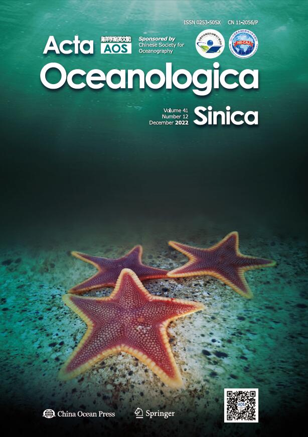
The study area (a) and the locations of the sampling stations (b). Black triangle markers are the sampling stations; red dotted lines represent the rang of table reefs.
| Citation: | Xiaofan Hong, Zuozhi Chen, Jun Zhang, Yan’e Jiang, Yuyan Gong, Yancong Cai, Yutao Yang. Construction and analysis of a coral reef trophic network for Qilianyu Islands, Xisha Islands[J]. Acta Oceanologica Sinica, 2022, 41(12): 58-72. doi: 10.1007/s13131-022-2047-8

|
The complex habitat composed of reef-building corals in the coral reef ecosystem is the main reason for its extremely high level of biodiversity and primary productivity (Knowlton, 2001). The large number of shelters, breeding grounds and nursery grounds in the ecosystem of coral reefs provide suitable habitats for various marine organisms with different living habits (Botha et al., 2013). However, coral reefs are currently under threat and deteriorating worldwide due to numerous influences of anthropogenic activities and climate change (Hoegh-Guldberg et al., 2007), which has prompted multifaceted conservation and restoration efforts (Baums, 2008).
Coral reefs in the South China Sea (SCS) cover an area of approximately 3.72×10⁴ km2, with tropical reefs therein accounting for nearly 5% of the total global area of coral reefs (Wang and Guan, 2020). The richness of corals in this region (571 species) is comparable to that in the “Coral Triangle” (Huang et al., 2015). Coral reef ecosystems in the SCS have abundant biological resources, with at least 3 600 fish species (Shao et al., 2008) (more than one-third of these are reef fish) having been reported from them. Coral reefs on the Xisha Islands of the central part of SCS are located more than 400 km from mainland China and are isolated from terrestrial nutrient influence via runoff through rivers and drains. As the main tropical fishing ground in China, there are more than 400 species of oceanic fish and coral reef fish in the coral reefs of the Xisha Islands, it is the important fishing ground for catching commercial fish such as tuna, mackerel, snapper, bonito, flying fish, shark and grouper. Moreover, as part of the Xisha Islands, Qilianyu Islands also as the site of the largest spawning ground for green turtle (Chelonia mydas) in China (Zhang et al., 2020b), more than 40 species of birds occur there, and the surrounding waters are rich in high-quality and valuable seafoods (Yang, 2017). Despite all of this, the numbers and density of coral reef fish in the waters surrounding the Qilianyu Islands have recently trended down because of anthropogenic disturbance and natural environment variation (Li et al., 2017), such as overfishing, destructive fishing, ocean acidification, ocean warming, typhoon damage, and outbreaks of crown-of-thorns starfish (Wu et al., 2011), these factors also chiefly responsible for serious declines in the SCS coral reef fishery resources (Zhang et al., 2020a). Continuing degradation of coral reef ecosystems has generated substantial interest in how management and restoration can support reef resilience (MacNeil et al., 2015). Many measures can be taken to reduce the threats affecting coral reef ecosystems. Confronting large-scale threats requires a major scaling-up of management and restoration efforts based on an improved understanding of the ecological processes that underlie reef resilience (Bellwood et al., 2004). Focusing in ecosystem assessment of coral reef, the lack of knowledge of the structure and function about coral reef ecosystems is one of the main problems for conserving the marine organisms living in coral reefs. Thus, in an effort to assess the health state and sustainable fishery of coral reef, modeling the compositions of coral reef ecosystem and their interaction trajectories should be necessary.
Models are increasingly used to improve our understanding of marine ecosystem functioning and address applied questions in the field of fishery management (Walters and Martell, 2004). Although, it is customary in ecosystem models to mix together what is inherent in physiological growth with counter-effects imposed by interactions with other species and self-limitation, ecosystem-based modeling methods which take into consideration characteristics of both the environment and organisms provide an effective tool to appraise the status of coral reef ecosystems. Model development involves computer software modeling (Bello-Pineda et al., 2006), dynamics simulation (Ippolito et al., 2016; Melbourne-Thomas et al., 2011), hyper-spectral remote sensing and radiation transmission modeling (Petit et al., 2017), mathematics (Jokiel, 2016; Li et al., 2014; Spillman and Alves, 2009), and assessment and monitoring of the various components of the coral reef ecosystem (González-Rivero et al., 2014; Heenan et al., 2017). Such models may improve understanding of the present-day status and dynamics of an ecosystem, can improve scientific theories, and they can guide measures to protect and restore coral reef ecosystems. As there are no standardized criteria for designing food web models in terms of grouping strategy and pedigree, it is frequently difficult to compare different food webs (Pérez-Ruzafa et al., 2020). The reconstruction of trophic pathways plays a fundamental role in understanding the structure and function of ecosystems (Pimm et al., 1991). Ecopath with Ecosim (EwE) provides an overview of an ecosystem’s trophic state, and can represent aquatic food webs (Christensen and Walters, 2004). Ecopath model was first used to simulate a coral reef ecosystem by Polovina (1984), and has since been developed and integrated into the EwE software package; it has now been used extensively in various aquatic ecosystems (Christensen and Pauly, 1992; Heymans et al., 2016). The operating principle of the Ecopath component in EwE is based on thermodynamics. The ecosystem is simplified by constructing a food web, with various ecosystem characteristics quantified through modeling. This can both reflect the characteristics and nutritional relationships of a specific ecosystem in a certain period as the static state of the food web mass balance, and it also serve as a starting point for more dynamic ecosystem models (Odum, 1969; Christensen and Pauly, 1992). Exploring the trajectory of energy flow could facilitate our understanding of ecosystem respondence and resilience to external disturbance. The SCS provides an excellent natural laboratory to reveal the ecology responses and variation tendency of coral reef ecosystem under changeable environmental conditions over a large spatial scale.
Most research on coral reef habitat in the SCS has focused on benthic algae (Chen et al., 2019; Wu et al., 2021), hermatypic coral communities (Li et al., 2018), coral-associated organism (Li et al., 2020; Zhang et al., 2020a), symbiotic microorganism of coral (Chen et al., 2021; Qin et al., 2021), and sediment layers (Yang, 2019). In the previous studies, the main aims were to assess how environmental factors (e.g., seawater environmental parameters, coral reef fish diversity and zooxanthellae density) across a large spatial scale can correlate or control the geographical distribution of coral reef. Because ecosystem-level management of coral reef fish has received limited attention, knowledge of the structure and ecological significance of coral reefs in the SCS is fragmentary. Therefore, given that ecosystem-based modeling methods provide effective tools for assessing the status of coral reef ecosystems, our research aims became to: (1) generate a preliminary trophic model for the Qilianyu Islands coral reef (QICR) to identify the main ecosystem trophic interaction pathways and trophic functioning, and (2) assess the status of this ecosystem and its maturity.
Qilianyu Islands, comprising Zhaohu Island, West Shoal, North Island, Center Island, South Island, North Shoal, South Shoal, West-New Shoal and East-New Shoal, are located in the northeastern part of the Xuande Islands (part of the Xisha Islands) in the central SCS (16°55′–17°00′N, 112°12′–112°21′E) (Fig. 1), belong to tropical coral reef regions with a high reef coral diversity and numerous coral species. The islands area is about 1.32 km2, the area of surrounding reef flat about 25 km2, surrounding water depth is mostly shallower than 20 m, and mean annual surface sea temperature 26.8℃. Because of the tropical monsoon climate, these islands are affected by 8–10 typhoons annually, with precipitation concentrated in summer and autumn (May–November); the tide is irregularly diurnal (Yang, 2017). Currents around the Qilianyu Islands are primarily wind-driven, with their direction changing with that of monsoon winds; currents between islands are influenced by tides (Yang, 2019).
We construct an Ecopath model to represent an average annual situation (2018–2019) for the QICR ecosystem with EwE 6.5 software (Christensen et al., 2005). In the Ecopath model, functional groups with similar trophic level (TL), life history and niche characteristics must be comprehensively considered (Pauly et al., 2000), and all functional groups must include basic processes of energy and material flow in the ecosystem (Christensen and Pauly, 1992). Ecopath model comprises two main equations—the first, Eq. (1), defines the balance between the input and output of each functional group to ensure that the ecotrophic efficiency (EE) does not exceed 1; Eq. (2) defines the thermodynamics of the functional groups. The expressions of Eq. (1) and Eq. (2) are
| $$ {B}_{i}\cdot {\left(P/B\right)}_{i}\cdot {{\rm{EE}}}_{i}={Y}_{i}+{\sum _{j=1}^{n}{B}_{j}\cdot \left(Q/B\right)_{j}}\cdot {{\rm{DC}}}_{ij}+{B}_{i}\cdot {{\rm{BA}}}_{i}+{E}_{i} , $$ | (1) |
| $$ {Q}_{i}={P}_{i}+{R}_{i}+{U}_{i} ,$$ | (2) |
where Bi is the biomass of group i; (P/B)i is the production of group i per unit biomass, equal to the total mortality rate of group i; EEi is the ecotrophic efficiency of group i, defined as the fraction of production that is consumed within the system or removed by fishers; Yi is the total fishery catch rate of group i; (Q/B)j is the consumption rate of group j per unit biomass; DCij is the fraction of prey i in the average diet of predator j; BAi is the biomass accumulation rate of group i; Ei is the net migration rate (immigration and emigration); Qi is the consumption of group i; Ri is the respiration of group i; and Ui is the unassimilated food of group i (Christensen et al., 2008).
Recognition of Ecopath functional groups requires consideration of shifts in the habitat of life history stages and/or diet. Thus, functional groups are represented as single biomass pools or multi-stanza functional groups (Walters et al., 2008). In this study, components in the Ecopath model for the QICR ecosystem can be divided into 21 functional groups (Table 1), 7 groups are fish groups; 7 groups are invertebrate groups, and the rest 6 groups are, turtles, zooplankton, phytoplankton, macroalgae, turf, and detritus, which cover the energy flow process of each ecosystem trophic level. Except for the results of field investigation, these functional groups are also selected based on characteristics of ecology, biosystematics, diets of species, and species distributions in the QICR area (Li et al., 2020). The species of fish are assigned to functional groups according to similar ecological characteristics (e.g., diet, predators, body sizes, and metabolic requirements), and the group names of carnivorous fish functional groups are assigned based on size (small, medium and large).
| Group name | Composition of dominant species |
| Chondrichthyes | ray, skate, shark |
| Large carnivorous fish | Aprion virescens, Pristipomoides filamentosus, Aphareus rutilans, large grouper, etc. |
| Medium carnivorous fish | Labridae, Lethrinidae, Priacanthidae, Mullidae, etc. |
| Small carnivorous fish | Holocentridae, Apogonidae, Cephalopholis, Epinephelus merra, etc. |
| Omnivorous fish | Pomacentridae, Balistidae, etc. |
| Coral-eating fish | Scaridae, Chaetodontidae, etc. |
| Herbivorous fish | Pomacanthidae, Acanthuridae, Siganus, etc. |
| Turtles | Chelonia mydas, Eretmochelys imbricata, Dermochelys coriacea, etc. |
| Crown-of-thorns starfish | Acanthaster planci |
| Giant triton | Charonia tritonis |
| Other echinoderms | urchin, cucumber, brittle star, starsish |
| Other mollusca | bivalve, snail, etc. |
| Crustaceans | crab & shrimp |
| Coral | Pocillopora damicornis, Pocillopora verrucosa, Acropora humilis, Porites lutea, etc. |
| Zooplankton | copepoda, planula, juvenile fish, etc. |
| Small benthic invertebrates | polychaeta, etc. |
| Macroalgae | coralline algae |
| Turf | turf |
| Phytoplankton | Bacillariopyta, Pyrrophyta, Chrysophyta, Cyanophyta, etc. |
| Detritus | particulate organic carbon & dissolved organic carbon |
 DownLoad:
CSV
DownLoad:
CSV
Biomass data for QICR coral reef fish is based on a 2019 shallow-water fishery-resource survey by the R/V Nanfengin. Fish species richness is based on collections of species made from ground cages, hand fishing and other operations. Biomass of each coral reef fish functional group is estimated from acoustic signals. Acoustic detection used a Simrad EK60 echosounder with 38 kHz and 120 kHz split-beam transducers (Zhang et al., 2016); data were collected from the surface to the seabed. Besides, some model parameters used in this study would also apply to other coral reef Ecopath models with similar ecosystem characteristics. Chondrichthyes biomass was obtained from Huang et al. (2009). Phytoplankton biomass (g/m2) was calculated following Brown et al. (1991) and Shang et al. (2018), based on the SCS chlorophyll a (Chl a) concentration (mg/m3) (Ke et al., 2018). Benthic producer (turf and macroalgae) biomass was estimated from empirical data and Wabnitz et al. (2010). Detrital biomass was calculated following Pauly et al. (1993), as a function of primary production and euphotic depth (Tang et al., 2007).
A lack of biomass data for corals, Acanthaster planci and Charonia tritonis, necessitated using output parameters of similar models; to balance our model EE values for each were set at 0.70, 0.30 and 0.95, respectively (Wabnitz et al., 2010; Cáceres et al., 2016; Ruiz et al., 2016; Du et al., 2020). These values were input into the model to calculate the biomass of missing functional groups. The biomass of other functional groups (other invertebrates) referenced models for adjacent seas or similar ecosystems (Du et al., 2015, 2020; Xie et al., 2019).
Methods used to estimate P/B include assessment of population resources, and estimation using natural mortality (M) and fishing mortality. According to bioenergy theory, the ratio of production (P)/consumption (Q), P/Q, is assumed to range of 0.1–0.3. Under assumptions of mass-balance trophic models, the P/B of “fishes” equals the instantaneous rate of total mortality (Z) (Allen, 1971). The Q/B for each fish functional group was estimated following Palomares and Pauly (1998); P/B and Q/B of some functional groups were estimated based on parameters in Fishbase (
The catch of QICR coral reef fish and some invertebrates was estimated from fishery data. Because a diet matrix is important for Ecopath simulation, the diets of different functional groups (Table 2) were reconstructed from stomach content analysis, published literature, and Fishbase (
| No. | Prey (predator) | 1 | 2 | 3 | 4 | 5 | 6 | 7 | 8 | 9 | 10 | 11 | 12 | 13 | 14 | 15 | 16 |
| 1 | chondrichthyes | 0.01 | 0 | 0 | 0 | 0 | 0 | 0 | 0 | 0 | 0 | 0 | 0 | 0 | 0 | 0 | 0 |
| 2 | large carnivorous fish | 0.05 | 0.008 | 0 | 0 | 0 | 0 | 0 | 0 | 0 | 0 | 0 | 0 | 0 | 0 | 0 | 0 |
| 3 | medium carnivorous fish | 0.14 | 0.1 | 0.009 | 0 | 0 | 0 | 0 | 0 | 0 | 0 | 0 | 0 | 0 | 0 | 0 | 0 |
| 4 | small carnivorous fish | 0.12 | 0.12 | 0.13 | 0.03 | 0.019 | 0 | 0 | 0 | 0 | 0 | 0 | 0 | 0 | 0 | 0 | 0 |
| 5 | omnivorous fish | 0.12 | 0.05 | 0.06 | 0.02 | 0.01 | 0 | 0 | 0 | 0 | 0 | 0 | 0 | 0.005 | 0 | 0 | 0 |
| 6 | coral-eating fish | 0.1 | 0.05 | 0.04 | 0.01 | 0.06 | 0 | 0 | 0 | 0 | 0 | 0 | 0 | 0 | 0 | 0 | 0 |
| 7 | herbivorous fish | 0.1 | 0.19 | 0.16 | 0.03 | 0.05 | 0 | 0 | 0 | 0 | 0 | 0 | 0 | 0.005 | 0 | 0 | 0 |
| 8 | turtles | 0.001 | 0 | 0 | 0 | 0 | 0 | 0 | 0 | 0 | 0 | 0 | 0 | 0 | 0 | 0 | 0 |
| 9 | crown-of-thorns starfish | 0 | 0.001 | 0.001 | 0 | 0.001 | 0 | 0 | 0 | 0 | 0.15 | 0 | 0 | 0.001 | 0 | 0 | 0 |
| 10 | giant triton | 1×10⁻⁵ | 0.000 5 | 0 | 0 | 0 | 0 | 0 | 0 | 0 | 0 | 0 | 0 | 0 | 0 | 0 | 0 |
| 11 | other echinoderms | 0 | 0.06 | 0.06 | 0.05 | 0.05 | 0 | 0 | 0 | 0 | 0.4 | 0 | 0 | 0.005 | 0 | 0 | 0 |
| 12 | other mollusca | 0.05 | 0.1 | 0.12 | 0.1 | 0.1 | 0 | 0 | 0.1 | 0 | 0.3 | 0 | 0.01 | 0.05 | 0 | 0 | 0 |
| 13 | crustaceans | 0.12 | 0.12 | 0.14 | 0.15 | 0.12 | 0 | 0 | 0.05 | 0 | 0 | 0 | 0 | 0.012 | 0 | 0 | 0 |
| 14 | coral | 0 | 0 | 0 | 0 | 0.05 | 0.4 | 0.1 | 0 | 0.8 | 0 | 0.05 | 0.06 | 0 | 0 | 0 | 0 |
| 15 | zooplankton | 0 | 0 | 0 | 0.28 | 0.1 | 0 | 0.05 | 0.1 | 0 | 0.15 | 0.15 | 0.25 | 0.2 | 0.1 | 0.01 | 0.1 |
| 16 | small benthic invertebrates | 0 | 0.05 | 0.18 | 0.2 | 0.1 | 0 | 0 | 0 | 0 | 0 | 0.05 | 0 | 0.133 | 0 | 0 | 0 |
| 17 | macroalgae | 0 | 0 | 0 | 0 | 0.13 | 0.3 | 0.3 | 0.3 | 0.07 | 0 | 0.2 | 0.2 | 0.1 | 0 | 0.05 | 0 |
| 18 | turf | 0 | 0 | 0 | 0 | 0.11 | 0.15 | 0.3 | 0.4 | 0.03 | 0 | 0.15 | 0.16 | 0.135 | 0 | 0.09 | 0 |
| 19 | phytoplankton | 0 | 0 | 0 | 0.03 | 0 | 0 | 0.1 | 0 | 0.1 | 0 | 0.12 | 0.22 | 0.154 | 0.3 | 0.6 | 0.15 |
| 20 | detritus | 0 | 0 | 0 | 0.1 | 0.1 | 0.15 | 0.15 | 0 | 0 | 0 | 0.28 | 0.1 | 0.2 | 0.4 | 0.25 | 0.75 |
| Import | 0.189 | 0.150 05 | 0.1 | 0 | 0 | 0 | 0 | 0.05 | 0 | 0 | 0 | 0 | 0 | 0.2 | 0 | 0 | |
| Sum | 1.000 01 | 0.999 55 | 1 | 1 | 1 | 1 | 1 | 1 | 1 | 1 | 1 | 1 | 1 | 1 | 1 | 1 |
DownLoad:
CSV
A pre-balance (PREBAL) diagnostic was used to check model consistency before balancing or running (Link, 2010). Checked indicators included biomass distribution, biomass ratios, vital rate distribution, vital rate ratios, and total production and removals.
According to thermodynamics, the Ecopath model after a PREBAL diagnostic is adjusted to reach a state of equilibrium. Output parameters requiring adjustment include: EE (<1.0), gross good conversion efficiency (P/Q, 0.1–0.3), net efficiency (NE, NE−P/Q>0), respiration/assimilation biomass (R/AS, <1.0), respiration/biomass (R/B, fish: 1–10; high conversion efficiency population: 50–100), and production/respiration (P/R, <1.0 or >1.0) (Link, 2010; Heymans et al., 2016).
A sensitivity analysis was performed to test how small variations in input data affect model output parameters (Steel et al., 2009). The sensitivity of output parameters to input data depends on degrees of association between functional groups. It is proposed that all basic input parameters change by steps of 10% within ±50%. Sensitivity was calculated following Christensen et al. (2005) as
| $$ ({\rm{estimated}} \;{\rm{parameter}} - {\rm{original}}\; {\rm{parameter}})/ {\rm{original}} \;{\rm{parameter}}. $$ | (3) |
The MTI of the Ecopath model quantifies the direct and indirect trophic effects between functional groups, assesses the positive or negative impact of changes in biomass of one functional group on all other components in the coral reef ecosystem, and analyzes interactions between functional groups and fishing activity (Ulanowicz and Puccia, 1990); it is calculated as follows:
| $$ {{\rm{MTI}}}_{{{ji}}}={{\rm{DC}}}_{ji}-{{\rm{FC}}}_{ij} , $$ | (4) |
where MTIji is the interaction between the impacting functional group j and the impacted functional group i, DCji is the fraction of prey j in the diet of predator i, and FCij is a host composition term giving the proportion of the predation on i because of j as a predator.
Keystone analyses are based on MTI to identify functional groups in the food web with high overall effects and relatively low biomass. This index is calculated following Libralato et al. (2006),
| $$ {\varepsilon }_{i}=\sqrt{\sum _{j\ne i}^{n}{{\rm{MTI}}}_{ij}^{2}} , $$ | (5) |
| $$ {{\rm{KS}}}_{i}=\mathrm{log}_{10}\left[{\varepsilon }_{i}\left(1-{p}_{i}\right)\right] , $$ | (6) |
where
According to the balanced results of the Ecopath model, the overall characteristic parameters of the ecosystem, calculated by network analysis to reflect the size, stability, and maturity of the QICR ecosystem, are used. Total system throughput (TST), which comprises the sums of all consumption, all exports, all respiratory flows, and all flows into detritus, can be used to quantify the ecological scale and “metabolic level” of an ecosystem (Finn, 1976; Ortiz et al., 2015). System descriptive indices such as ratios of total primary production/total respiration (TPP/TR) and total primary production/total biomass (TPP/TB), Finn’s cycling index (FCI), and Finn's mean path length (MPL), characterize ecosystem maturity (Odum, 1969; Finn, 1976; Christensen et al., 2008). The closer TPP/TR is to 1, the more stable is an ecosystem. Cycling of matter is also a critical process in natural ecosystem functioning because it can facilitate homeostatic control of the magnitude of flows (Odum, 1969); FCI and MPL increase with ecosystem maturity. Food web complexity and omnivory are often used to assess ecosystem stability (Landi et al., 2018); the connectance index (CI) is a ratio of the number of actual links to number of possible links for a given food web, and the system omnivory index (SOI) is the average omnivory index of all consumers weighted by the logarithm of each consumer’s food intake (Christensen et al., 2008). Both CI and SOI indicate the complexity of internal ecosystem connections; when their values approach 1, the relationship within the food web formed by functional groups is more likely to be complex, and the ecosystem more stable. Ascendency (A) integrates both size and organization (the number and diversity of interactions between ecosystem components) (Christensen et al., 2008); the relative overhead (O/C) is used as an index of ecosystem resilience (Heymans, 2003).
According to PREVAL diagnostics, QICR biomass estimates span 5 orders of magnitude (biomass in an aquatic ecosystem typically covers 5–7 orders of magnitude (Link, 2010)). Additionally, because the log-scale biomass slope falls by −0.117 across all trophic levels, QICR ecosystem primary productivity and functional group biomass of low TLs are high (a general range is −0.05 to −0.1 (Link, 2010)). P/B, Q/B and R/B values for each functional group decrease with increased TL, and biomass and production values for each functional group of consumers also exceed those of primary producers. Total consumption removals for each consumer functional group are lower than production values, and all have total consumption removals below the sum of human removals (e.g., catch), except for turtles and carnivorous fish (medium and large).
Sensitivity analysis reveals relationships between EE and biomass for each functional group to be most sensitive, with a 50% increase in biomass of a functional group resulting in an average decrease of about 30.11% in its estimated EE value. A linear relationship is also apparent between input parameters (i.e., P/B, Q/B, EE) of each functional group. Compared with other sensitivity relationships, the EE of phytoplankton is most sensitive when its biomass decreases, while the EE of turf has the highest relative increase with an increase in its biomass.
QICR Ecopath model functional group input and output parameters are listed in Table 3. The TL for each functional group is consistent with the fundamental laws of ecology, ranging 1.00–3.80 (Fig. 2), with half concentrated in TLs II or III. Among consumers, chondrichthyes (3.80) and large carnivorous fish (3.57) occupy the top two food web positions. The mean TL for coral reef fish is 2.92, with the interval between functional groups 2.16–3.57. For invertebrates, the giant triton (3.34), crown of thorns starfish (2.90), and coral (2.13) have the highest TL values; except for primary producers and detritus, the TL of zooplankton is the lowest. The EE of functional groups ranges 0.187–0.981, with the highest value for omnivorous fish and the lowest for detritus. The range in GE for each functional group is 0.053–0.446, with “other mollusca” (0.446) and zooplankton (0.313) having the highest values.
| No. | Group name | TL | B/(t·km−2·a−1) | P:B/(a−1) | Q:B/(a−1) | Un. Q | Catch | EE | P/Q | NE | OI |
| 1 | chondrichthyes | 3.80 | 0.097 | 0.25 | 4.72 | 0.20 | − | 0.189 | 0.05 | 0.07 | 0.41 |
| 2 | large carnivorous fish | 3.57 | 0.430 | 0.79 | 6.64 | 0.20 | 0.200 | 0.723 | 0.12 | 0.15 | 0.30 |
| 3 | medium carnivorous fish | 3.42 | 3.781 | 1.00 | 8.50 | 0.20 | 2.500 | 0.830 | 0.12 | 0.15 | 0.16 |
| 4 | small carnivorous fish | 3.07 | 1.700 | 4.00 | 13.50 | 0.20 | 0.800 | 0.942 | 0.30 | 0.37 | 0.22 |
| 5 | omnivorous fish | 2.84 | 1.103 | 4.50 | 16.30 | 0.20 | 1.500 | 0.981 | 0.28 | 0.35 | 0.40 |
| 6 | coral-eating fish | 2.45 | 1.415 | 2.40 | 20.00 | 0.20 | 0.200 | 0.878 | 0.12 | 0.15 | 0.30 |
| 7 | herbivorous fish | 2.16 | 8.156 | 3.00 | 28.00 | 0.40 | 1.800 | 0.397 | 0.11 | 0.18 | 0.15 |
| 8 | turtles | 2.32 | 0.020 | 0.14 | 3.50 | 0.20 | 0.002 | 0.878 | 0.04 | 0.05 | 0.29 |
| 9 | crown-of-thorns starfish | 2.90 | 0.485 | 1.20 | 5.00 | 0.20 | − | 0.300 | 0.24 | 0.30 | 0.20 |
| 10 | giant triton | 3.34 | 0.002 | 1.22 | 4.08 | 0.20 | 0.001 | 0.950 | 0.30 | 0.37 | 0.07 |
| 11 | other echinoderms | 2.26 | 3.035 | 2.20 | 7.80 | 0.20 | 0.500 | 0.786 | 0.28 | 0.35 | 0.21 |
| 12 | other mollusca | 2.33 | 8.700 | 2.50 | 5.60 | 0.20 | 6.000 | 0.955 | 0.45 | 0.56 | 0.24 |
| 13 | crustaceans | 2.46 | 4.300 | 3.20 | 28.00 | 0.25 | 0.500 | 0.904 | 0.11 | 0.15 | 0.31 |
| 14 | coral | 2.13 | 19.574 | 3.00 | 10.00 | 0.20 | − | 0.700 | 0.30 | 0.38 | 0.13 |
| 15 | zooplankton | 2.01 | 3.510 | 76.00 | 242.50 | 0.30 | − | 0.416 | 0.31 | 0.45 | 0.01 |
| 16 | small benthic invertebrates | 2.10 | 3.911 | 12.00 | 60.00 | 0.25 | − | 0.629 | 0.20 | 0.27 | 0.09 |
| 17 | macroalgae | 1.00 | 22.000 | 18.00 | − | − | − | 0.375 | − | − | − |
| 18 | turf | 1.00 | 30.000 | 25.00 | − | − | − | 0.239 | − | − | − |
| 19 | phytoplankton | 1.00 | 8.817 | 231.00 | − | − | − | 0.324 | − | − | − |
| 20 | detritus | 1.00 | 315.000 | − | − | − | − | 0.187 | − | − | 0.24 |
| Note: B: biomass; OI: omnivory index; TL: trophic level; P/B: production/biomass; Q/B: consumption/biomass; Un. Q: unassim. consumption; EE: ecotrophic efficiency; P/Q: production/consumption; NE: net efficiency. Values in bold are estimated by the present model. − reprsents no data. | |||||||||||
DownLoad:
CSV

Network analysis confirmed compartmental throughput of the 20 functional groups in a Lindeman spine with 5 integrated TL (Fig. 3). The “all flow” of each TL decreases substantially with increased TL (Table 4). Flows within TLs I and II generate 77.24% and 19.93% of throughput, respectively, consistent with principles of an energy pyramid. As the major source of energy, the flow of consumption by TL I predators accounts for 87.40% of the sum for consumption by predators, and the flow to detritus accounts for 75.27% of the sum for flow to detritus, demonstrating fairly inefficient energy utilization of TL I; most energy is stored as detritus in low TLs, which cannot be transferred upward.

| Trophic level | |||||
| Consumption by predators | Export | Flow to detritus | Respiration | Throughput | |
| V | 0.070 | 0.125 | 0.406 | 1.196 | 1.798 |
| IV | 1.650 | 1.220 | 6.121 | 15.040 | 24.030 |
| III | 23.730 | 5.445 | 56.840 | 110.500 | 196.500 |
| II | 194.700 | 7.207 | 658.500 | 713.600 | 1 574.000 |
| I | 1 533.000 | 2 371.000 | 2 195.000 | 0.000 | 6 099.000 |
| Sum | 1 754.000 | 2 385.000 | 2 916.000 | 840.400 | 7 896.000 |
DownLoad:
CSV
The transfer efficiency of a TL is the ratio of output and ingested energy to its throughput. Transfer efficiency indicates the energy efficiency of a TL in an ecosystem. The geometric mean of the transfer efficiency (mTE) for the food web from TLs II–IV is 13.15% (above the Lindeman trophic transfer efficiency (10%)) (Lindeman, 1942), with 13.15% from primary producers and 13.14% from detritus (Table 5). The proportion of total flow originating from detritus (45%) and primary producers (55%) indicates that the QICR ecosystem is dominated by a grazing food chain.
| Source | Trophic level | |||
| II | III | IV | V | |
| Producer | 12.37 | 15.53 | 11.84 | 11.1 |
| Detritus | 13.64 | 13.73 | 12.13 | 10.43 |
| All flows | 12.83 | 14.84 | 11.94 | 10.87 |
| Note: Proportion of total flow originating from detritus: 0.45; transfer efficiencies (mTE, calculated as geometric mean for TL II–IV); from primary producers: 13.15%; from detritus: 13.14%; total: 13.15%. | ||||
DownLoad:
CSV
The niche overlap index mainly describes niche partitioning between functional groups; it is based on similarities in, for example, predation, competition, and environmental adaptation. Corals and zooplankton have the lowest degree of predatory overlap of all functional groups, but a high degree of prey overlap; herbivorous and small carnivorous fish have similar predators, but their prey is quite different; crustaceans and other echinoderms have high prey and predator overlaps, indicating their very similar niches, especially when competing as predators (Fig. 4).

MTI analysis (Fig. 5) reveals primary producers have a positive effect on most functional groups, benthic algae (turf and macroalgae) have a negative effect on coral, and coral has an obvious positive effect on coral-eating fish and crown of thorns starfish. The negative effects of fishing activity and the functional group “crustaceans” on the giant triton are the result of direct and indirect impacts, respectively; the giant triton also has a significant negative effect on the crown of thorns starfish, which it preys upon. Fishing activity has an obvious negative effect on medium and large carnivorous fish, while an increase in fishing intensity is associated with a positive impact on the biomass of omnivorous fishes, small carnivorous fishes, and crown of thorns starfish. This indirectly suggests that fishing activities in this area affect the coral reef ecosystem.

Based on the keystone index (KS) and relative total impact (RTI), it is determined that the key functional groups in the QICR ecosystem include corals (KS=−0.197, RTI=1.00), crustaceans (KS=−0.144, RTI=0.981), and herbivorous fish (KS=−0.159, RTI=0.981) (Fig. 6). The high KS and RTI of these functional groups imply that they play important roles in the QICR ecosystem.

QICR ecosystem characteristics are presented in Table 6. TST was 7 952 t/(km2·a), of which 22.76% is due to consumption and 10.57% to respiration; 29.99% and 36.68% of this originates in backflows to exports and detritus, respectively. TPP/TR is 3.79, TPP/TB 26.30, FCI 3.64%, and MPL 2.47. The mean trophic level of catches (TLc) is relatively low (2.62). The total overhead for this ecosystem is 22 977 t/(km2·a), with a total ascendency (A) accounting for 27.71% of total capacity (C).
| Area | Qilianyu Islands | Hawaii Island | Cocos Island | Darwin &Wolf Island | Nanwan Bay | Uvea Atoll | Caribbean Sea | |
| Cayos Cochinos | Media Luna | |||||||
| Group number | 20 | 26 | 31 | 32 | 18 | 25 | 22 | 21 |
| Sum of all consumption/(t·km−2·a−1) | 1 810 | 5 332 | 22 978 | 8 880 | 8 373 | 292 | 31 013 | 27 381 |
| Sum of all exports/(t·km−2·a−1) | 2 385 | 520 | 20 | 344 | 16 200 | 185 | 81 700 | 9 779 |
| Sum of all respiratory flows/(t·km−2·a−1) | 840 | 3 477 | 12 050 | 5 278 | 4 629 | 86 | 17 096 | 16 264 |
| Sum of all flows into detritus/(t·km−2·a−1) | 2 916 | 1 700 | 6 136 | 2 151 | 20 115 | 346 | 90 | 17 881 |
| TST/(t·km−2·a−1) | 7 952 | 11 030 | 41 184 | 16 652 | 49 317 | 909 | 220 232 | 71 305 |
| Sum of all production/(t·km−2·a−1) | 3 642 | − | 978 | 5 235 | 21 553 | 325 | 10 6510 | 31 684 |
| TLc | 2.62 | 2.59 | 3.55 | 3.02 | 2.40 | 3.50 | 3.64 | 2.97 |
| GE | 0.00 4 | 0.000 09 | 2.00×10⁻⁶ | 0.001 | 0.000 36 | 0.000 15 | 1.01×10⁻⁹ | 1.20×10⁻⁵ |
| Net p.p./(t·km−2·a−1) | 3 182.73 | 3 895.09 | 4 583.59 | 3 408.00 | 20 199.00 | 265.30 | 98 796.00 | 26 043.00 |
| TPP/TR | 3.79 | 1.12 | 0.38 | 0.65 | 4.40 | 3.10 | 5.78 | 1.60 |
| NSP/(t·km−2·a−1) | 2 342.30 | 417.78 | −7 466.37 | −1 898.00 | 15 570.00 | 179.40 | 81 700.00 | 9 779.00 |
| TPP/TB | 26.30 | 5.57 | 2.32 | 3.64 | 9.90 | 19.95 | 11.82 | 10.21 |
| TB:TST/(a−1) | 0.015 | 0.06 | 0.05 | 0.06 | 0.04 | 0.01 | 0.04 | 0.04 |
| Total catch/(t·km−2·a−1) | 14.003 | 0.350 | 0.010 | 3.841 | 7.300 | 0.039 | 1.00×10⁻⁴ | 0.311 |
| CI | 0.33 | − | 0.17 | 0.15 | − | − | 0.30 | 0.26 |
| SOI | 0.21 | − | 0.40 | 0.32 | − | − | 0.21 | 0.20 |
| FCI/% | 3.64 | 6.13 | 6.50 | 4.75 | 3.50 | − | 1.60 | 6.95 |
| MPL | 2.47 | − | − | − | − | − | 6.65 | 5.65 |
| A:C/% | 27.71 | 31.50 | 24.80 | 29.80 | − | − | 47.00 | 31.00 |
| mTE/% | 13.15 | − | 12.20 | 10.70 | 7.80 | − | − | − |
| Note: GE: Gross efficiency (total catch/net p.p.); net p.p.: calculated total net primary production; NSP: net system production; TST: total system throughput; TLc: mean trophic level of the catch; TPP/TR: total primary production/total respiration; NSP: net system production; TPP/TB: total primary production/total biomass; TB/TST: total biomass/total throughput; CI: connectance index; SOI: system omnivory index; FCI: Finn's cycling index; MPL: Finn's mean path length; A/C: ascendency/capacity; mTE: mean transfer efficiencies. −represent no data. | ||||||||
DownLoad:
CSV
To evaluate the status of the QICR ecosystem, we refer to coral reef Ecopath models for the Atlantic and Pacific. The QICR ecosystem has a relatively reduced total biomass, but its gross efficiency and total catch are higher than reported for other coral reef ecosystems. The mean trophic level of QICR catch (2.62) is significantly lower than values for coral reef ecosystems in the Caribbean Sea (Cayos Cochinos Islands and Media Luna Archipelago) (Cáceres et al., 2016), Cocos Island (Gaither et al., 2011), Galapagos Islands (Darwin and Wolf Islands) (Ruiz et al., 2016), and Uvea Atoll (Bozec et al., 2004), but similar to Hawaii Island (2.59) (Wabnitz et al., 2010) and Nanwan Bay, Taiwan (2.40) (Liu et al., 2009). The proportion of TST components in the Ecopath model of QICR ecosystem differs in some regards from those in other Ecopath models. The sum of flows into detritus represents the highest proportion of TST (36.68%) in the QICR, similar to Ecopath models for coral reef ecosystems in the Nanwan Bay and Uvea Atoll. The QICR TPP/TR was also closest to a value for Uvea Atoll, however, TPP/TB and total biomass/total system throughput (TB/TST) are significantly higher or lower than values for most other coral reef ecosystem models. Comparison of model results indicates that the QICR CI and SOI are closest to those of the Caribbean Sea. The A/C of this study was in the range of 24.8%–31.0% reported for other coral reef ecosystem models, excepting the Cayos Cochinos.
The QICR ecosystem was supported primarily by input of flows and materials from detritus and primary producers (phytoplankton, turf and macroalgae) (Table 4), with the four functional groups at TL I all having lower EE values (Table 3). Although only a small flow of detritus and primary producers enter to other TL, but a substantial proportion flow of them was exported from the ecosystem or was returned to the detritus pool. Coral reef ecosystems are among the most biodiverse ecosystems in the world and have great ecological importance and economic value (McCook et al., 2009). The oligotrophic nature and high biological productivity of seawater in coral reef habitats are notable features of coral reef ecosystems (Adey and Goertemiller, 1987), and their biological productivity is 50–100 times that of the surrounding tropical oceans. As the second largest producer in coral reef ecosystems, detritus is an essential feature of ecosystem development (Arias-González et al., 1997). Natural sources of marine detritus include animals, phytoplankton, bacteria and blue green algae, periphyton, submerged aquatic vegetation, intertidal macrophytes, river borne detritus, beach and shore material, terrestrial detritus and atmospheric deposition (Darnell, 1967). Accumulated detritus is buried in sediment and is further decomposed or mineralized by micro-benthic heterotrophs (Nixon et al., 1986; Chen and Qiu, 2010). Sediment is also widely considered to influence coral reef ecosystems (Bahr et al., 2020), significantly affecting turf productivity (Tebbett and Bellwood, 2020), and regulating the feeding of fish and spatial scales of ecosystem function delivery (Tebbett et al., 2020). In the other way, bacteria can either be attached to particulate detritus, or aggregated interstitially within the spaces of sediment and particulate matter (Mason and Varnell, 1996). Furthermore, like many coral reef fisheries, the catch in the reef fish of QICR is dominated by herbivorous fishes (Tebbett and Bellwood, 2020) (Table 3) , which provide important grazing functions for coral reef ecosystems and improve the ability of coral reefs to self-repair under climate change-related disturbances, they are generally considered to be one of the key contributors to maintaining coral reef ecosystem health (Bellwood et al., 2004; Bozec et al., 2016; Hughes et al., 2007). In addition, the higher biomass and catch of herbivorous fish in our model suggest that the QICR ecosystem may be due to coral reef degradation (such as coral–algal phase shift) and overfishing, which leading to a decrease in the biomass of traditional top predators in habitats, while the proportion of herbivorous fish biomass increased (Ainsworth and Mumby, 2015; Arias-González et al., 2004; Darling and D’Agata, 2017).
The niche overlap analysis provides evidence that the functional group of crustaceans and other echinoderms both have a high similarity for their prey and predator (Fig 4). They are the main components of benthic invertebrate communities in coral reef, both have the highest degree of similarity in the niche in the QICR ecosystem. Different with reef fish, benthic invertebrates have relatively single food sources due to the limitation of habitat topography and their own mobility, the benthic food web structure of coral reef formed by them is the main way for detritus to enter the energy flow of ecosystem. In general, niche overlap results in functional redundancy (Mouillot et al., 2013) and intensifies competition among functional groups with similar niches. However, in a coral reef ecosystem with high biodiversity and bottom-up control (Frank et al., 2007), we suggest that the combination of niche overlap between crustaceans and other echinoderms improves resistance and repairability of QICR ecosystem.
A keystone functional group is a species or species assemblage that has a controlling effect in a key position of food web. There is little doubt that corals represent a keystone group in the QICR ecosystem. Historically, coral cover in the Xisha Islands exceeded 50%. However, because of coral disease, ocean warming and acidification, overfishing, and crown of thorns starfish outbreaks, coral cover has dropped to about 15% (Li et al., 2019b). Present-day coral cover in QICR has recovered slowly since being substantially reduced in 2007 (Li et al., 2018). Combined with results of keystone analysis, corals continue to dominate the QICR ecosystem trophic structure, despite the reef habitat being seriously degraded. This indicates that corals have provided functional complementarity (Brandl et al., 2016) for the coral reef ecosystem. Due to the nature of Ecopath model and the limitation of dataset, microbiomes that symbiosis with corals are not set as functional groups in this study, such as endosymbiotic Symbiodiniaceae (formerly named zooxanthellae), bacteria, viruses, fungi, and archaea. In the construction of Ecopath model, therefore, we empirically integrated these microbiomes within the coral functional group, treating the two as a whole. As the critical parts of the coral reef ecosystem, the symbiotic microbiomes of coral can transfer their photosynthetically derived nutrients for daily metabolism of corals. But corals can also be heterotrophic, as they feed on a variety of sources, including suspended particulate matter (Mills et al., 2004), dissolved organic compounds (Godinot et al., 2011), phytoplankton (Ferrier-Pagès et al., 2011), and zooplankton (Houlbrèque et al., 2003). During the growth of corals, the heterotrophic feeding of corals provides adequate phosphorus, nitrogen and other micronutrients that are deficient in photosynthetic products (Xu et al., 2021). This is one of the main reasons why we consider corals as consumer rather than primary producer. Moreover, according to the output results of QICR model, the TL for functional group of coral (TL=2.13) may not be able to completely reflect the characteristics that corals possess the capability for mixotrophy (autotrophic and heterotrophic), but at least we can better understand the rough trophic status of corals between primary producers and primary consumers in ecosystem from the energy flow diagram. Different carbon and nitrogen sources have distinct stable isotopic compositions (Wu et al., 2021), stable isotope analysis has emerged as one of most powerful tools for tracing organic matter in food webs (Thomas Larsen) and indicating organism diet and trophic position for organisms. In the future study, using stable isotope analysis to reveal the food source of corals and the role of symbiotic microbiomes (Luo et al., 2019), and accurately reflect the trophic level of corals in the ecosystem, is one of the important tasks to improve the construction of coral reef ecosystem model.
MTI analysis reveals coral has a significant effect on coral-eating fish and the coral-eating crown of thorns starfish (Li et al., 2019a) (Fig. 5), while the giant triton has a significant negative effect on the crown of thorns starfish through predation. Early reports of large-scale outbreaks of this starfish were made on the Great Barrier Reef, Australia (Chesher, 1969). Waters in and surrounding the QICR and throughout the SCS have been severely damaged by outbreaks of this starfish (Huang et al., 2012; Reimer et al., 2019). Because of this, many coral reefs may collapse through bioerosion and currents, which possibly influences their ecological function by reducing reef structural complexity (Fabricius et al., 2010). The giant triton, one of few natural predators for crown of thorns starfish, occurs mainly throughout Indo-Pacific tropical coral reef waters (Zhang et al., 2013). The market value of these tritons has resulted in the overexploitation of wild populations, potentially leading to local extinction (Russo et al., 1990). This has affected crown of thorn starfish populations (Zhang et al., 2013). Li et al. (2019b) reported large-scale outbreaks of this starfish on other coral reefs around the Qilianyu Islands from 2018, despite the existence of potential barriers to its dispersal such as strong currents and depths between islands (Muallil et al., 2020). Because the density of crown of thorns starfish is inversely proportional to the number of living corals (Wilmes et al., 2020), the Ecopath model described herein may underestimate crown of thorns starfish biomass and overestimate that of the giant triton. MTI analysis also demonstrated fishing activity to have variable negative effects on corals and the giant triton, but a positive effect on the crown of thorns starfish. Consequently, fisheries can both directly and indirectly affect the function and status of corals. Overfishing degrades biological resources and modifies coral reef food webs (e.g., the giant triton plays an important role in maintaining a complex balance in the coral reef ecosystem (Glynn and Enochs, 2011)). A reduction in coral biomass leads to algal overgrowth (Hodgson, 1999), which reduces reef structure complexity and potentially affects the feeding of coral reef fish (McCormick et al., 2017), and the coral–algal phase shift would reduce biodiversity and ecosystem maturity (Ainsworth and Mumby, 2015). Although, there is no doubt that the potential importance of individual herbivorous species in removing macroalgae from coral reefs (Mantyka and Bellwood, 2007), the process of macroalgal removal would be strongly influenced by coral reef conditions (Chong-Seng et al., 2014). Cheal et al. (2010) suggested that coral reefs could lose resilience even under relatively low fishing pressure on herbivorous fishes. Nevertheless, coral communities in the SCS have dramatically declined over the past several decades (Yu, 2012). The coral cover in the central SCS has declined from over 70% in the 1980s (Hughes et al., 2007) to 16% in 2015 (Chen et al., 2019). Likewise, investigation data show that the coral cover in the ecological monitoring area of the Xisha Islands decreased from about 70% to less than 15% from 2001 to 2019 (Li et al., 2019b), as the consequence of frequent anthropogenic activities (overfishing and destructive fishing) and recurrent natural events (ocean warming, typhoon damage, and outbreaks of crown-of-thorns starfish). Consequently, it is necessary to take some measures for identification and protection of ecosystem components that are critical for the prevention of coral–algal phase shift in QICR ecosystem.
To evaluate the status of the QICR ecosystem, results from it are compared with Ecopath models for coral reefs elsewhere throughout the Atlantic and Pacific (Table 6). Features of TST components for these models vary. The sum of flows into detritus for the QICR ecosystem represented the highest proportion of TST (36.68%), similar to models for coral reefs in the Nanwan Bay and Uvea Atoll. The estimated QICR TPP/TR (2.981) is closest to a value for Uvea Atoll, which indicates that increased organic matter caused the TPP to exceed the TR; the QICR TPP/TB ratio (26.1) is significantly higher than values for most other coral reef ecosystems, which also indicates that the QICR ecosystem is tending to develop towards resource accumulation. Both TPP/TR and TPP/TB values suggest that the QICR ecosystem is immature, or in a state of “poor stability”. Low CI and SOI values imply that redundancy in and the resistance of the food web are weak; both values are closest to those for the Caribbean Sea. FCI (4.80) and MPL (2.58) values indicate that the proportion of productivity devoted to material cycle is low. Compared with other models, the QICR has the highest gross efficiency, which indicates that the production efficiency of fishery resources is higher. Collectively, the QICR ecosystem maturity level is generally lower than for most other coral reef ecosystems, being most similar to the Nanwan Bay. The QICR is situated in an open water area, and of all other reefs for which Ecopath models are available, is geographically closest to the Nanwan Bay. Therefore, QICR and the Nanwan Bay coral reef ecosystems may be similar because of comparable anthropogenic disturbance (mainly intensive fishing), but potentially also because the coral reef ecosystems in and around the SCS might have relatively similar ecological characteristics.
Furthermore, in the Ecopath model of coral reef ecosystems involved in the comparative analysis, A/C in other models ranges 24.8%–31.0% of output results, except for the Cayos Cochinos model; the A/C of the QICR Ecopath model is 27.71%, which indicates that this ecosystem has considerable development potential, and spaces for buffer interference. However, about the source of overhead, the internal flow and import accounted for 59.07% and 0.39% of total capacity, respectively. This indicates that the ecosystem has strong internal buffer spaces to effectively buffer it from external interference, but the buffer capacity for external importation is weak. The QICR ecosystem is likely vulnerable to external importation. Eutrophication is a main driver of algal distribution on coral reefs (Huang et al., 2020). Seawater around the Qilianyu Islands is affected by complex and strong hydrodynamics and convergences can easily form (Yang, 2019). Therefore, in the ecosystem of QICR, if a large amount of nutrients input exceeds the threshold, it may cause large fluctuations in the structure and function of the ecosystem. Although some researches highlight anthropogenic nutrient deposition as an important nutrient source for coral reef (Chen et al., 2019; Kim et al., 2014), there is increasing evidence that anthropogenic activities have bring additional material inputs to coral reefs (Zhang et al., 2020a). Anyway, those are undoubtedly direct evidence that climate change and anthropogenic activities are affecting the habitat of coral reef and should be a cause for concern.
Compared with other coral reef models, although the total biomass of the QICR ecosystem is relatively reduced, its total efficiency and total catch are higher than those reported by other models, indicating that the fishery resource exploitation efficiency in the study area is higher. In general, differences in ecosystem type influence ecological characteristics (Heymans et al., 2011), however, TLc can indicate major differences in fishery protection between ecosystems (Albouy et al., 2010). The TLc of the QICR model (2.62) is significantly lower than that for coral reefs in the Caribbean Sea (Cayos Cochinos Islands and Media Luna Archipelago), Galapagos Islands (Darwin and Wolf Islands), and Uvea Atoll, while those for Hawaii Island (2.59) and Nanwan Bay (2.40) are relatively close. According to the results of Nanwan Bay model, Liu et al. (2009) suggests an overfished status would lead to the mean trophic level of the catch, matter cycling, and trophic transfer efficiency are extremely reduced. In addition, given that coral reefs are often overfished (Mumby et al., 2006), climate change induced degradation will limit the ability of coral reefs to exert its ecosystem functions (Dove et al., 2020). The reasons that TLc of the QICR model is also lower than values from the northern SCS (2.93) (Chen and Qiu, 2010) are possibly that the combined effects of climate change (Alva-Basurto and Arias-González, 2014) and fishing activities (Pauly et al., 1998) have down the food web. On the one hand, climate change is a big one that one of the most important threats facing coral reefs on a global scale (Lough, 2011), ocean acidification and ocean warming are two climate-related impacts to coral reefs. If large amounts of anthropogenic CO2 from the atmosphere are dissolved in seawater that would causes the lowering of the ocean’s pH (ocean acidification) (Hoegh-Guldberg et al., 2007). And ocean acidification reduces the calcium carbonate in the seawater, making it difficult for corals to form skeletons (Anthony et al., 2008). The results of Eyre et al. (2018) showed that under the action of ocean acidification, it is expected that by circa 2050 CE, reef sediments globally will transition from net precipitation to net dissolution. In addition, ocean warming water caused by global warming would prompt corals to release the zooxanthellae, and then make corals experience different degrees of bleaching (Gates, 1990), all of which would eventually lead to large-scale death of corals and the degradation of coral reef ecosystem (Cook et al., 1990). According to the Status of Coral Reefs of the World: 2020 report produced by the Global Coral Reef Monitoring Network, the total amount of corals in the world’s coral reefs gradually declined by 14% since 2009, which is more than all the coral currently living on Australia’s coral reefs. There are evidences that sea surface temperatures in the SCS increased in the last several decades since the middle of the twentieth century (Jiao et al., 2015). On the other hand, “Fishing down the food web” refers to the decreasing of the catch size due to the depletion of previous catch size (Pauly et al., 1998; Pauly and Palomares, 2005), for example, excessive artisanal fishing pressure may be the main hindrance to develop ecosystem quality in the shelf slope area (Karim et al., 2019). Except for overfishing, destructive fishing such as cyanide fishing and blast fishing are often considered one of the most destructive human activities on coral reef ecosystems (Fox and Caldwell, 2006; Mak et al., 2005). Of the more than 1 000 species of coral reef fish assessed by the International Union for Conservation of Nature, 8% of them are threatened with extinction (Hixon and Randall, 2019). Consequently, anthropogenic activities can indirectly and/or directly act to homogenize and simplify ecosystems, by the climate change and fishing activities that aforementioned discussions, artificially favoring stress-tolerant species and forcing the ecosystem into an earlier successional state (Williams et al., 2015).
EwE is used to construct an Ecopath model for the QICR ecosystem. This represents the first study to construct an Ecopath model for a coral reef ecosystem in the SCS and proffers the first comparative analysis of ecosystem structure and function in the QICR and other coral reefs. The QICR ecosystem has a high energy transfer efficiency (mTE=13.15%) compared with other models, but it is also degrading and has low ecological stability. Direct and indirect effects of climate change and anthropogenic disturbance (e.g., fishing) are the main reasons for QICR degradation. Policy should incorporate an ecosystem-based approach to fisheries management for coral reef fish resources and for protection and reparation of reefs to improve their resilience and resistance, to realize sustainable development of coral reef fishery resources. Although this study has conducted a comprehensive assessment and analysis of the ecological characteristics of the QICR ecosystem, there are still some deficiencies. As a static model, Ecopath model does not consider the impact on the model caused by changes in environmental factors, such as the temporal and spatial factors in seasonal changes, therefore, the results predicted by the model must be used with caution in combination with the field survey results. In addition, the ecological status simulated based on Ecopath model mainly emphasizes the theoretical boundary, while lack the consideration about the impact of the growth and development of organisms at various trophic levels on the ecosystem structure, so it is difficult to scientifically reflect the actual conditions of the ecosystem. The study here can provide a background for the follow-up research on the dynamic changes of the QICR ecosystem. Long-term monitoring research and precise quantitative techniques are needed in order to provide a more comprehensive scientific theoretical basis for the development and management strategies of coral reef fisheries.
Acknowledgements: We wish to acknowledge the South China Sea Fisheries Research Institute for providing the data used for this study, and Steve O’Shea from Edanz Group (|
Adey W H, Goertemiller T. 1987. Coral reef algal turfs: master producers in nutrient poor seas. Phycologia, 26(3): 374–386. doi: 10.2216/i0031-8884-26-3-374.1
|
|
Ainsworth C H, Mumby P J. 2015. Coral–algal phase shifts alter fish communities and reduce fisheries production. Global Change Biology, 21(1): 165–172. doi: 10.1111/gcb.12667
|
|
Albouy C, Mouillot D, Rocklin D, et al. 2010. Simulation of the combined effects of artisanal and recreational fisheries on a Mediterranean MPA ecosystem using a trophic model. Marine Ecology Progress Series, 412: 207–221. doi: 10.3354/meps08679
|
|
Allen K R. 1971. Relation between production and biomass. Journal of the Fisheries Research Board of Canada, 28(10): 1573–1581. doi: 10.1139/f71-236
|
|
Alva-Basurto J C, Arias-González J E. 2014. Modelling the effects of climate change on a Caribbean coral reef food web. Ecological Modelling, 289: 1–14. doi: 10.1016/j.ecolmodel.2014.06.014
|
|
Anthony K R N, Kline D I, Diaz-Pulido G, et al. 2008. Ocean acidification causes bleaching and productivity loss in coral reef builders. Proceedings of the National Academy of Sciences of the United States of America, 105(45): 17442–17446. doi: 10.1073/pnas.0804478105
|
|
Arias-González J E, Delesalle B, Salvat B, et al. 1997. Trophic functioning of the Tiahura reef sector, Moorea Island, French Polynesia. Coral Reefs, 16(4): 231–246. doi: 10.1007/s003380050079
|
|
Arias-González J E, Nuñez-Lara E, González-Salas C, et al. 2004. Trophic models for investigation of fishing effect on coral reef ecosystems. Ecological Modelling, 172(2–4): 197–212,
|
|
Bahr K D, Rodgers K S, Jokiel P L, et al. 2020. Pulse sediment event does not impact the metabolism of a mixed coral reef community. Ocean & Coastal Management, 184: 105007. doi: 10.1016/j.ocecoaman.2019.105007
|
|
Baums I B. 2008. A restoration genetics guide for coral reef conservation. Molecular Ecology, 17(12): 2796–2811. doi: 10.1111/j.1365-294X.2008.03787.x
|
|
Bello-Pineda J, Ponce-Hernández R, Liceaga-Correa M A. 2006. Incorporating GIS and MCE for suitability assessment modelling of coral reef resources. Environmental Monitoring and Assessment, 114(1–3): 225–256,
|
|
Bellwood D R, Hughes T P, Folke C, et al. 2004. Confronting the coral reef crisis. Nature, 429(6994): 827–833. doi: 10.1038/nature02691
|
|
Botha E J, Brando V E, Anstee J M, et al. 2013. Increased spectral resolution enhances coral detection under varying water conditions. Remote Sensing of Environment, 131: 247–261. doi: 10.1016/j.rse.2012.12.021
|
|
Bozec Y M, Gascuel D, Kulbicki M. 2004. Trophic model of lagoonal communities in a large open atoll (Uvea, Loyalty Islands, New Caledonia). Aquatic Living Resources, 17(2): 151–162. doi: 10.1051/alr:2004024
|
|
Bozec Y M, O’Farrell S, Bruggemann J H, et al. 2016. Tradeoffs between fisheries harvest and the resilience of coral reefs. Proceedings of the National Academy of Sciences of the United States of America, 113(16): 4536–4541. doi: 10.1073/pnas.1601529113
|
|
Brandl S J, Emslie M J, Ceccarelli D M, et al. 2016. Habitat degradation increases functional originality in highly diverse coral reef fish assemblages. Ecosphere, 7(11): e01557. doi: 10.1002/ecs2.1557
|
|
Brown P C, Painting S J, Cochrane K L. 1991. Estimates of phytoplankton and bacterial biomass and production in the northern and southern Benguela ecosystems. South African Journal of Marine Science, 11(1): 537–564. doi: 10.2989/025776191784287673
|
|
Cáceres I, Ortiz M, Cupul-Magaña A L, et al. 2016. Trophic models and short-term simulations for the coral reefs of Cayos Cochinos and Media Luna (Honduras): a comparative network analysis, ecosystem development, resilience, and fishery. Hydrobiologia, 770(1): 209–224. doi: 10.1007/s10750-015-2592-7
|
|
Cheal A J, MacNeil M A, Cripps E, et al. 2010. Coral–macroalgal phase shifts or reef resilience: links with diversity and functional roles of herbivorous fishes on the Great Barrier Reef. Coral Reefs, 29(4): 1005–1015. doi: 10.1007/s00338-010-0661-y
|
|
Chen Zuozhi, Qiu Yongsong. 2010. Assessment of the food-web structure, energy flows, and system attribute of northern South China Sea ecosystem. Acta Ecologica Sinica, 30(18): 4855–4865
|
|
Chen Zuozhi, Xu Shannan, Qiu Yongsong. 2015. Using a food-web model to assess the trophic structure and energy flows in Daya Bay, China. Continental Shelf Research, 111: 316–326. doi: 10.1016/j.csr.2015.08.013
|
|
Chen Xiaoyan, Yu Kefu, Huang Xueyong, et al. 2019. Atmospheric nitrogen deposition increases the possibility of macroalgal dominance on remote coral reefs. Journal of Geophysical Research: Biogeosciences, 124(5): 1355–1369. doi: 10.1029/2019jg005074
|
|
Chen Biao, Yu Kefu, Liao Zhiheng, et al. 2021. Microbiome community and complexity indicate environmental gradient acclimatisation and potential microbial interaction of endemic coral holobionts in the South China Sea. Science of the Total Environment, 765: 142690. doi: 10.1016/j.scitotenv.2020.142690
|
|
Chesher R H. 1969. Destruction of Pacific corals by the sea star Acanthaster planci. Science, 165(3890): 280–283. doi: 10.1126/science.165.3890.280
|
|
Chong-Seng K M, Nash K L, Bellwood D R, et al. 2014. Macroalgal herbivory on recovering versus degrading coral reefs. Coral Reefs, 33(2): 409–419. doi: 10.1007/s00338-014-1134-5
|
|
Christensen V, Pauly D. 1992. ECOPATH II—a software for balancing steady-state ecosystem models and calculating network characteristics. Ecological Modelling, 61(3–4): 169–185,
|
|
Christensen V, Walters C J. 2004. Ecopath with Ecosim: methods, capabilities and limitations. Ecological Modelling, 172(2–4): 109–139,
|
|
Christensen V, Walters C J, Pauly D. 2005. Ecopath with Ecosim: A User’s Guide. Vancouver: University of British Columbia
|
|
Christensen V, Walters C, Pauly D, et al. 2008. Ecopath with Ecosim Version 6 User Guide. Vancouver: University of British Columbia
|
|
Cook C B, Logan A, Ward J, et al. 1990. Elevated temperatures and bleaching on a high latitude coral reef: the 1988 Bermuda event. Coral Reefs, 9(1): 45–49. doi: 10.1007/BF00686721
|
|
Darling E S, D’Agata S. 2017. Coral reefs: fishing for sustainability. Current Biology, 27(2): R65–R68. doi: 10.1016/j.cub.2016.12.005
|
|
Darnell R M. 1967. Organic detritus in relation to the estuarine ecosystem. In: Lauff G H, ed. Estuaries. Washington: American Association for the Advancement of Science, 376–382
|
|
Dove S G, Brown K T, Van Den Heuvel A, et al. 2020. Ocean warming and acidification uncouple calcification from calcifier biomass which accelerates coral reef decline. Communications Earth & Environment, 1(1): 55. doi: 10.1038/s43247-020-00054-x
|
|
Du Jianguo, Makatipu P C, Tao L S R, et al. 2020. Comparing trophic levels estimated from a tropical marine food web using an ecosystem model and stable isotopes. Estuarine, Coastal and Shelf Science, 233: 106518,
|
|
Du Feiyan, Wang Xuehui, Lin Zhaojin. 2015. The characteristics of summer zooplankton community in the Meiji coral reef, Nansha Islands, South China Sea. Acta Ecologica Sinica, 35(4): 1014–1021
|
|
Eyre B D, Cyronak T, Drupp P, et al. 2018. Coral reefs will transition to net dissolving before end of century. Science, 359(6378): 908–911. doi: 10.1126/science.aao1118
|
|
Fabricius K E, Okaji K, De’ath G. 2010. Three lines of evidence to link outbreaks of the crown-of-thorns seastar Acanthaster planci to the release of larval food limitation. Coral Reefs, 29(3): 593–605. doi: 10.1007/s00338-010-0628-z
|
|
Ferrier-Pagès C, Hoogenboom M, Houlbrèque F. 2011. The role of plankton in coral trophodynamics. In: Dubinsky Z, Stambler N, eds. Coral Reefs: An Ecosystem in Transition. Dordrecht: Springer,
|
|
Finn J T. 1976. Measures of ecosystem structure and function derived from analysis of flows. Journal of Theoretical Biology, 56(2): 363–380. doi: 10.1016/S0022-5193(76)80080-X
|
|
Fox H E, Caldwell R L. 2006. Recovery from blast fishing on coral reefs: a tale of two scales. Ecological Applications, 16(5): 1631–1635. doi: 10.1890/1051-0761(2006)016[1631:RFBFOC]2.0.CO;2
|
|
Frank K T, Petrie B, Shackell N L. 2007. The ups and downs of trophic control in continental shelf ecosystems. Trends in Ecology & Evolution, 22(5): 236–242. doi: 10.1016/j.tree.2007.03.002
|
|
Gaither M R, Bowen B W, Bordenave T R, et al. 2011. Phylogeography of the reef fish Cephalopholis argus (Epinephelidae) indicates Pleistocene isolation across the Indo-Pacific Barrier with contemporary overlap in the Coral Triangle. BMC Evolutionary Biology, 11: 189. doi: 10.1186/1471-2148-11-189
|
|
Gates R D. 1990. Seawater temperature and sublethal coral bleaching in Jamaica. Coral Reefs, 8(4): 193–197. doi: 10.1007/BF00265010
|
|
Glynn P W, Enochs I C. 2011. Invertebrates and their roles in coral reef ecosystems. In: Dubinsky Z, Stambler N, eds. Coral Reefs: An Ecosystem in Transition. Dordrecht: Springer, 273–325
|
|
Godinot C, Houlbrèque F, Grover R, et al. 2011. Coral uptake of inorganic phosphorus and nitrogen negatively affected by simultaneous changes in temperature and pH. PLoS ONE, 6(9): e25024. doi: 10.1371/journal.pone.0025024
|
|
González-Rivero M, Bongaerts P, Beijbom O, et al. 2014. The catlin seaview survey-kilometre-scale seascape assessment, and monitoring of coral reef ecosystems. Aquatic Conservation: Marine and Freshwater Ecosystems, 24(S2): 184–198. doi: 10.1002/aqc.2505
|
|
Heenan A, Williams I D, Acoba T, et al. 2017. Long-term monitoring of coral reef fish assemblages in the western central Pacific. Scientific Data, 4: 170176. doi: 10.1038/sdata.2017.176
|
|
Heymans J. 2003. Comparing the Newfoundland marine ecosystem models using Information Theory. Fisheries Centre Research Reports, 11(5): 62–71
|
|
Heymans J J, Coll M, Libralato S, et al. 2011. Ecopath theory, modeling, and application to coastal ecosystems. Treatise on Estuarine and Coastal Science, 9: 93–113
|
|
Heymans J J, Coll M, Link J S, et al. 2016. Best practice in Ecopath with Ecosim food-web models for ecosystem-based management. Ecological Modelling, 331: 173–184. doi: 10.1016/j.ecolmodel.2015.12.007
|
|
Hixon M A, Randall J E. 2019. Coral reef fishes. Encyclopedia of Ocean Sciences, 2: 142–150
|
|
Hodgson G. 1999. A global assessment of human effects on coral reefs. Marine Pollution Bulletin, 38(5): 345–355. doi: 10.1016/S0025-326X(99)00002-8
|
|
Hoegh-Guldberg O, Mumby P J, Hooten A J, et al. 2007. Coral reefs under rapid climate change and ocean acidification. Science, 318(5857): 1737–1742. doi: 10.1126/science.1152509
|
|
Houlbrèque F, Tambutté E, Ferrier-Pagès C. 2003. Effect of zooplankton availability on the rates of photosynthesis, and tissue and skeletal growth in the scleractinian coral Stylophora pistillata. Journal of Experimental Marine Biology and Ecology, 296(2): 145–166. doi: 10.1016/S0022-0981(03)00259-4
|
|
Huang Zirong, Chen Zuozhi, Zeng Xiaoguang. 2009. Species composition and resources density of Chondrichthyes in the continental shelf of northern South China Sea. Journal of Oceanography in Taiwan Strait, 28(1): 38–44
|
|
Huang Danwei, Licuanan W Y, Hoeksema B W, et al. 2015. Extraordinary diversity of reef corals in the South China Sea. Marine Biodiversity, 45(2): 157–168. doi: 10.1007/s12526-014-0236-1
|
|
Huang Jianhong, Wang Fengxia, Zhao Hongwei, et al. 2020. Reef benthic composition and coral communities at the Wuzhizhou Island in the South China Sea: the impacts of anthropogenic disturbance. Estuarine, Coastal and Shelf Science, 243: 106863,
|
|
Huang Hui, Zhang Chenglong, Yang Jianhui, et al. 2012. Scleractinian coral community characteristics in Zhubi reef sea area of Nansha Islands. Journal of Oceanography in Taiwan Strait, 31(1): 79–84
|
|
Hughes T P, Rodrigues M J, Bellwood D R, et al. 2007. Phase shifts, herbivory, and the resilience of coral reefs to climate change. Current Biology, 17(4): 360–365. doi: 10.1016/j.cub.2006.12.049
|
|
Ippolito S, Naudot V, Noonburg E G. 2016. Alternative stable states, coral reefs, and smooth dynamics with a kick. Bulletin of Mathematical Biology, 78(3): 413–435. doi: 10.1007/s11538-016-0148-2
|
|
Jiao Nianzhi, Chen Dake, Luo Yongming, et al. 2015. Climate change and anthropogenic impacts on marine ecosystems and countermeasures in China. Advances in Climate Change Research, 6(2): 118–125. doi: 10.1016/j.accre.2015.09.010
|
|
Jokiel P L. 2016. Predicting the impact of ocean acidification on coral reefs: evaluating the assumptions involved. ICES Journal of Marine Science, 73(3): 550–557. doi: 10.1093/icesjms/fsv091
|
|
Karim E, Liu Qun, Xue Ying, et al. 2019. Trophic structure and energy flow of the resettled maritime area of the Bay of Bengal, Bangladesh through ECOPATH. Acta Oceanologica Sinica, 38(10): 27–42. doi: 10.1007/s13131-019-1423-5
|
|
Ke Zhixin, Tan Yehui, Huang Liangmin, et al. 2018. Spatial distribution patterns of phytoplankton biomass and primary productivity in six coral atolls in the central South China Sea. Coral Reefs, 37(3): 919–927. doi: 10.1007/s00338-018-1717-7
|
|
Kim T W, Lee K, Duce R, et al. 2014. Impact of atmospheric nitrogen deposition on phytoplankton productivity in the South China Sea. Geophysical Research Letters, 41(9): 3156–3162. doi: 10.1002/2014gl059665
|
|
Knowlton N. 2001. Coral reef biodiversity-habitat size matters. Science, 292(5521): 1493–1495. doi: 10.1126/science.1061690
|
|
Landi P, Minoarivelo H O, Brännström Å, et al. 2018. Complexity and stability of ecological networks: a review of the theory. Population Ecology, 60(4): 319–345. doi: 10.1007/s10144-018-0628-3
|
|
Li Yuanjie, Chen Zuozhi, Zhang Jun, et al. 2020. Species and taxonomic diversity of Qilianyu Island reef fish in the Xisha Islands. Journal of Fishery Sciences of China, 27(7): 815–823
|
|
Li Yuanchao, Chen Shiquan, Zheng Xinqing, et al. 2018. Analysis of the change of hermatypic corals in Yongxing Island and Qilianyu Island in nearly a decade. Haiyang Xuebao (in Chinese), 40(8): 97–109
|
|
Li Yuanchao, Liang Jilin, Wu Zhongjie, et al. 2019a. Outbreak and prevention of Acanthaster planci. Ocean Development and Management, 36(8): 9–12
|
|
Li Xiong, Wang Hao, Zhang Zheng, et al. 2014. Mathematical analysis of coral reef models. Journal of Mathematical Analysis and Applications, 416(1): 352–373. doi: 10.1016/j.jmaa.2014.02.053
|
|
Li Yuanchao, Wu Zhongjie, Chen Shiquan, et al. 2017. Discussion of the diversity of the coral reef fish in the shallow reefs along the Yongxing and Qilianyu Island. Marine Environmental Science, 36(4): 509–516
|
|
Li Yuanchao, Wu Zhongjie, Liang Jilin, et al. 2019b. Analysis on the outbreak period and cause of Acanthaster planci in Xisha Islands in recent 15 years. Chinese Science Bulletin, 64(33): 3478–3484. doi: 10.1360/tb-2019-0152
|
|
Libralato S, Christensen V, Pauly D. 2006. A method for identifying keystone species in food web models. Ecological Modelling, 195(3–4): 153–171,
|
|
Lindeman R L. 1942. The trophic-dynamic aspect of ecology. Ecology, 23(4): 399–417. doi: 10.2307/1930126
|
|
Link J S. 2010. Adding rigor to ecological network models by evaluating a set of pre-balance diagnostics: a plea for PREBAL. Ecological Modelling, 221(12): 1580–1591. doi: 10.1016/j.ecolmodel.2010.03.012
|
|
Liu P J, Shao K T, Jan R Q, et al. 2009. A trophic model of fringing coral reefs in Nanwan Bay, southern Taiwan suggests overfishing. Marine Environmental Research, 68(3): 106–117. doi: 10.1016/j.marenvres.2009.04.009
|
|
Lough J M. 2011. Climate change and coral reefs. In: Hopley D, ed. Encyclopedia of Modern Coral Reefs. Encyclopedia of Earth Sciences Series. Dordrecht: Springer,
|
|
Luo Zhongyuan, Li Jiangtao, Jia Guodong. 2019. The geochemical significance of deep-water coral and their food source. Advances in Earth Science, 34(12): 1234–1242. doi: 10.11867/j.issn.1001-8166.2019.12.1234
|
|
MacNeil M A, Graham N A J, Cinner J E, et al. 2015. Recovery potential of the world’s coral reef fishes. Nature, 520(7547): 341–344. doi: 10.1038/nature14358
|
|
Mak K K W, Yanase H, Renneberg R. 2005. Cyanide fishing and cyanide detection in coral reef fish using chemical tests and biosensors. Biosensors and Bioelectronics, 20(12): 2581–2593. doi: 10.1016/j.bios.2004.09.015
|
|
Mantyka C S, Bellwood D R. 2007. Direct evaluation of macroalgal removal by herbivorous coral reef fishes. Coral Reefs, 26(2): 435–442. doi: 10.1007/s00338-007-0214-1
|
|
Mason P, Varnell L M. 1996. Detritus: mother nature’s rice cake. Wetlands Program Technical Report no. 96-10. Gloucester Point, Virginia: Virginia Institute of Marine Science, College of William and Mary,
|
|
McCook L J, Almany G R, Berumen M L, et al. 2009. Management under uncertainty: guide-lines for incorporating connectivity into the protection of coral reefs. Coral Reefs, 28(2): 353–366. doi: 10.1007/s00338-008-0463-7
|
|
McCormick M I, Barry R P, Allan B J M. 2017. Algae associated with coral degradation affects risk assessment in coral reef fishes. Scientific Reports, 7(1): 16937. doi: 10.1038/s41598-017-17197-1
|
|
Melbourne-Thomas J, Johnson C R, Fung T, et al. 2011. Regional-scale scenario modeling for coral reefs: a decision support tool to inform management of a complex system. Ecological Applications, 21(4): 1380–1398. doi: 10.1890/09-1564.1
|
|
Mills M M, Lipschultz F, Sebens K P. 2004. Particulate matter ingestion and associated nitrogen uptake by four species of scleractinian corals. Coral Reefs, 23(3): 311–323. doi: 10.1007/s00338-004-0380-3
|
|
Mouillot D, Graham N A J, Villéger S, et al. 2013. A functional approach reveals community responses to disturbances. Trends in Ecology & Evolution, 28(3): 167–177. doi: 10.1016/j.tree.2012.10.004
|
|
Muallil R N, Tambihasan A M, Enojario M J, et al. 2020. Inventory of commercially important coral reef fishes in Tawi-Tawi Islands, Southern Philippines: the Heart of the Coral Triangle. Fisheries Research, 230: 105640. doi: 10.1016/j.fishres.2020.105640
|
|
Mumby P J, Dahlgren C P, Harborne A R, et al. 2006. Fishing, trophic cascades, and the process of grazing on coral reefs. Science, 311(5757): 98–101. doi: 10.1126/science.1121129
|
|
Nixon S W, Oviatt C A, Frithsen J, et al. 1986. Nutrients and the productivity of estuarine and coastal marine ecosystems. Journal of the Limnological Society of Southern Africa, 12(1–2): 43–71,
|
|
Odum E P. 1969. The strategy of ecosystem development. Science, 164(3877): 262–270. doi: 10.1126/science.164.3877.262
|
|
Ortiz M, Berrios F, Campos L, et al. 2015. Mass balanced trophic models and short-term dynamical simulations for benthic ecological systems of Mejillones and Antofagasta Bays (SE Pacific): comparative network structure and assessment of human impacts. Ecological Modelling, 309–310: 153–162,
|
|
Palomares M L D, Pauly D. 1998. Predicting food consumption of fish populations as functions of mortality, food type, morphometrics, temperature and salinity. Marine and Freshwater Research, 49(5): 447–453. doi: 10.1071/MF98015
|
|
Pauly D, Christensen V, Dalsgaard J, et al. 1998. Fishing down marine food webs. Science, 279(5352): 860–863. doi: 10.1126/science.279.5352.860
|
|
Pauly D, Christensen V, Walters C. 2000. Ecopath, Ecosim, and Ecospace as tools for evaluating ecosystem impact of fisheries. ICES Journal of Marine Science, 57(3): 697–706. doi: 10.1006/jmsc.2000.0726
|
|
Pauly D, Palomares M L D. 2005. Fishing down marine food web: it is far more pervasive than we thought. Bulletin of Marine Science, 76(2): 197–211
|
|
Pauly D, Soriano-Bartz M L, Palomares M L D. 1993. Improved construction, parametrization and interpretation of steady-state ecosystem models. In: Christensen V, Pauly D, eds. Trophic Models of Aquatic Ecosystems. Manila: ICLARM Conference Proceeding
|
|
Pérez-Ruzafa A, Morkune R, Marcos C, et al. 2020. Can an oligotrophic coastal lagoon support high biological productivity? Sources and pathways of primary production. Marine Environmental Research, 153: 104824. doi: 10.1016/j.marenvres.2019.104824
|
|
Petit T, Bajjouk T, Mouquet P, et al. 2017. Hyperspectral remote sensing of coral reefs by semi-analytical model inversion—Comparison of different inversion setups. Remote Sensing of Environment, 190: 348–365. doi: 10.1016/j.rse.2017.01.004
|
|
Pimm S L, Lawton J H, Cohen J E. 1991. Food web patterns and their consequences. Nature, 350(6320): 669–674. doi: 10.1038/350669a0
|
|
Polovina J J. 1984. Model of a coral reef ecosystem. Coral Reefs, 3(1): 1–11. doi: 10.1007/BF00306135
|
|
Qin Zhenjun, Yu Kefu, Chen Shuchang, et al. 2021. Microbiome of juvenile corals in the outer reef slope and lagoon of the South China Sea: insight into coral acclimatization to extreme thermal environments. Environmental Microbiology, 23(8): 4389–4404. doi: 10.1111/1462-2920.15624
|
|
Reimer J D, Kise H, Wee H B, et al. 2019. Crown-of-thorns starfish outbreak at oceanic Dongsha Atoll in the northern South China Sea. Marine Biodiversity, 49(6): 2495–2497. doi: 10.1007/s12526-019-01021-2
|
|
Ruiz D J, Banks S, Wolff M. 2016. Elucidating fishing effects in a large-predator dominated system: the case of Darwin and Wolf Islands (Galápagos). Journal of Sea Research, 107: 1–11. doi: 10.1016/j.seares.2015.11.001
|
|
Russo G F, Fasulo G, Toscano A, et al. 1990. On the presence of triton species (Charonia spp. ) (Mollusca Gastropoda) in the Mediterranean Sea: ecological considerations. Bollettino Malacologico, 26: 91–104
|
|
Shang Yiwei, Xiao Wupeng, Liu Xin, et al. 2018. Variations of pico-phytoplankton groups and carbon to chlorophyll-a ratios in the South China Sea at the SEATS station. Journal of Xiamen University (Natural Science), 57(6): 811–818
|
|
Shao K T, Ho H C, Lin P L, et al. 2008. A checklist of the fishes of southern Taiwan, northern South China Sea. The Raffles Bulletin of Zoology, 19: 233–271
|
|
Spillman C M, Alves O. 2009. Dynamical seasonal prediction of summer sea surface temperatures in the Great Barrier Reef. Coral Reefs, 28(1): 197–206. doi: 10.1007/s00338-008-0438-8
|
|
Steel E A, McElhany P, Yoder N J, et al. 2009. Making the best use of modeled data: multiple approaches to sensitivity analysis of a fish-habitat model. Fisheries, 34(7): 330–339. doi: 10.1577/1548-8446-34.7.330
|
|
Tang Shilin, Chen Chuqun, Zhan Haigang, et al. 2007. Retrieval of euphotic layer depth of South China Sea by remote sensing. Journal of Tropical Oceanography, 26(1): 9–15
|
|
Tebbett S B, Bellwood D R. 2020. Sediments ratchet-down coral reef algal turf productivity. Science of the Total Environment, 713: 136709. doi: 10.1016/j.scitotenv.2020.136709
|
|
Tebbett S B, Goatley C H R, Streit R P, et al. 2020. Algal turf sediments limit the spatial extent of function delivery on coral reefs. Science of the Total Environment, 734: 139422. doi: 10.1016/j.scitotenv.2020.139422
|
|
Ulanowicz R E, Puccia C J. 1990. Mixed trophic impacts in ecosystems. Coenoses, 5(1): 7–16
|
|
Wabnitz C C C, Balazs G, Beavers S, et al. 2010. Ecosystem structure and processes at Kaloko Honokohau, focusing on the role of herbivores, including the green sea turtle Chelonia mydas, in reef resilience. Marine Ecology Progress Series, 420: 27–44. doi: 10.3354/meps08846
|
|
Walters C J, Martell S J D. 2004. Fisheries Ecology and Management. Princeton: Princeton University Press
|
|
Walters C, Martell S J D, Christensen V, et al. 2008. An ecosim model for exploring gulf of Mexico ecosystem management options: implications of including multistanza life-history models for policy predictions. Bulletin of Marine Science, 83(1): 251–271
|
|
Wang Geng, Guan Xiaoxi. 2020. Research status and hot spot analysis of a coral reef ecosystem model. Acta Ecologica Sinica, 40(4): 1496–1503
|
|
Williams G J, Gove J M, Eynaud Y, et al. 2015. Local human impacts decouple natural biophysical relationships on Pacific coral reefs. Ecography, 38(8): 751–761. doi: 10.1111/ecog.01353
|
|
Wilmes J C, Schultz D J, Hoey A S, et al. 2020. Habitat associations of settlement-stage crown-of-thorns starfish on Australia’s Great Barrier Reef. Coral Reefs, 39(4): 1163–1174. doi: 10.1007/s00338-020-01950-6
|
|
Wu Zhongjie, Wang Daoru, Tu Zhigang, et al. 2011. The analysis on the reason of hermatypic coral degradation in Xisha. Acta Oceanologica Sinica, 33(4): 140–146
|
|
Wu Dan, Zhang Fenfen, Zhang Xiaodi, et al. 2021. Stable isotopes (δ13C and δ15 N) in black coral as new proxies for environmental record. Marine Pollution Bulletin, 164: 112007. doi: 10.1016/j.marpolbul.2021.112007
|
|
Xie Fuwu, Liang Jilin, Xing Kongmin, et al. 2019. Characteristics of zooplankton community structure in the eastern and southern offshore coral reef areas of Hainan in summer. Marine Sciences, 43(7): 87–95
|
|
Xu Shendong, Zhang Zhinan, Yu Kefu, et al. 2021. Spatial variations in the trophic status of Favia palauensis corals in the South China Sea: insights into their different adaptabilities under contrasting environmental conditions. Science China Earth Sciences, 64(6): 839–852. doi: 10.1007/s11430-020-9774-0
|
|
Yang Junyi. 2017. Spectral analysis and classification of coral reefs around Qilian Yu in the Xisha Islands (in Chinese)[dissertation]. Guangzhou: Guangzhou University
|
|
Yang Rui. 2019. The study of microbial communities and their potentiality to be environmental indicators of surface layer sediments in Xuande Atoll, the South China Sea (in Chinese)[dissertation]. Beijing: China University of Geosciences (Beijing)
|
|
Yu Kefu. 2012. Coral reefs in the South China Sea: their response to and records on past environmental changes. Science China Earth Sciences, 55(8): 1217–1229. doi: 10.1007/s11430-012-4449-5
|
|
Zhang Jun, Chen Guobao, Chen Zuozhi, et al. 2016. Application of hydroacoustics to investigate the distribution, diel movement, and abundance of fish on Zhubi Reef, Nansha Islands, South China Sea. Chinese Journal of Oceanology and Limnology, 34(5): 964–976. doi: 10.1007/s00343-016-5019-z
|
|
Zhang Jun, Chen Zuozhi, Dong Junde, et al. 2020a. Variation in the population characteristics of blue-striped snapper Lutjanus kasmira in the South China Sea in recent 20 years. Oceanologia et Limnologia Sinica, 51(1): 114–124
|
|
Zhang Ting, Lin Liu, Jian Li, et al. 2020b. Investigation of beach debris at spawning ground of Green Sea Turtles (Chelonia mydas) at Qilianyu Islands, northeastern Xisha Islands. Chinese Journal of Ecology, 39(7): 2408–2415
|
|
Zhang Lüping, Xia Jianjun, Peng Pengfei, et al. 2013. Characterization of embryogenesis and early larval development in the Pacific triton, Charonia tritonis (Gastropoda: Caenogastropoda). Invertebrate Reproduction & Development, 57(3): 237–246. doi: 10.1080/07924259.2012.753472
|


Figures(6) / Tables(6)

Supported by:
Beijing Renhe Information Technology Co. Ltd

Xiaofan Hong, Zuozhi Chen, Jun Zhang, Yan’e Jiang, Yuyan Gong, Yancong Cai, Yutao Yang. Construction and analysis of a coral reef trophic network for Qilianyu Islands, Xisha Islands[J]. Acta Oceanologica Sinica, 2022, 41(12): 58-72. doi: 10.1007/s13131-022-2047-8

| Group name | Composition of dominant species |
| Chondrichthyes | ray, skate, shark |
| Large carnivorous fish | Aprion virescens, Pristipomoides filamentosus, Aphareus rutilans, large grouper, etc. |
| Medium carnivorous fish | Labridae, Lethrinidae, Priacanthidae, Mullidae, etc. |
| Small carnivorous fish | Holocentridae, Apogonidae, Cephalopholis, Epinephelus merra, etc. |
| Omnivorous fish | Pomacentridae, Balistidae, etc. |
| Coral-eating fish | Scaridae, Chaetodontidae, etc. |
| Herbivorous fish | Pomacanthidae, Acanthuridae, Siganus, etc. |
| Turtles | Chelonia mydas, Eretmochelys imbricata, Dermochelys coriacea, etc. |
| Crown-of-thorns starfish | Acanthaster planci |
| Giant triton | Charonia tritonis |
| Other echinoderms | urchin, cucumber, brittle star, starsish |
| Other mollusca | bivalve, snail, etc. |
| Crustaceans | crab & shrimp |
| Coral | Pocillopora damicornis, Pocillopora verrucosa, Acropora humilis, Porites lutea, etc. |
| Zooplankton | copepoda, planula, juvenile fish, etc. |
| Small benthic invertebrates | polychaeta, etc. |
| Macroalgae | coralline algae |
| Turf | turf |
| Phytoplankton | Bacillariopyta, Pyrrophyta, Chrysophyta, Cyanophyta, etc. |
| Detritus | particulate organic carbon & dissolved organic carbon |
DownLoad:
CSV
| No. | Prey (predator) | 1 | 2 | 3 | 4 | 5 | 6 | 7 | 8 | 9 | 10 | 11 | 12 | 13 | 14 | 15 | 16 |
| 1 | chondrichthyes | 0.01 | 0 | 0 | 0 | 0 | 0 | 0 | 0 | 0 | 0 | 0 | 0 | 0 | 0 | 0 | 0 |
| 2 | large carnivorous fish | 0.05 | 0.008 | 0 | 0 | 0 | 0 | 0 | 0 | 0 | 0 | 0 | 0 | 0 | 0 | 0 | 0 |
| 3 | medium carnivorous fish | 0.14 | 0.1 | 0.009 | 0 | 0 | 0 | 0 | 0 | 0 | 0 | 0 | 0 | 0 | 0 | 0 | 0 |
| 4 | small carnivorous fish | 0.12 | 0.12 | 0.13 | 0.03 | 0.019 | 0 | 0 | 0 | 0 | 0 | 0 | 0 | 0 | 0 | 0 | 0 |
| 5 | omnivorous fish | 0.12 | 0.05 | 0.06 | 0.02 | 0.01 | 0 | 0 | 0 | 0 | 0 | 0 | 0 | 0.005 | 0 | 0 | 0 |
| 6 | coral-eating fish | 0.1 | 0.05 | 0.04 | 0.01 | 0.06 | 0 | 0 | 0 | 0 | 0 | 0 | 0 | 0 | 0 | 0 | 0 |
| 7 | herbivorous fish | 0.1 | 0.19 | 0.16 | 0.03 | 0.05 | 0 | 0 | 0 | 0 | 0 | 0 | 0 | 0.005 | 0 | 0 | 0 |
| 8 | turtles | 0.001 | 0 | 0 | 0 | 0 | 0 | 0 | 0 | 0 | 0 | 0 | 0 | 0 | 0 | 0 | 0 |
| 9 | crown-of-thorns starfish | 0 | 0.001 | 0.001 | 0 | 0.001 | 0 | 0 | 0 | 0 | 0.15 | 0 | 0 | 0.001 | 0 | 0 | 0 |
| 10 | giant triton | 1×10⁻⁵ | 0.000 5 | 0 | 0 | 0 | 0 | 0 | 0 | 0 | 0 | 0 | 0 | 0 | 0 | 0 | 0 |
| 11 | other echinoderms | 0 | 0.06 | 0.06 | 0.05 | 0.05 | 0 | 0 | 0 | 0 | 0.4 | 0 | 0 | 0.005 | 0 | 0 | 0 |
| 12 | other mollusca | 0.05 | 0.1 | 0.12 | 0.1 | 0.1 | 0 | 0 | 0.1 | 0 | 0.3 | 0 | 0.01 | 0.05 | 0 | 0 | 0 |
| 13 | crustaceans | 0.12 | 0.12 | 0.14 | 0.15 | 0.12 | 0 | 0 | 0.05 | 0 | 0 | 0 | 0 | 0.012 | 0 | 0 | 0 |
| 14 | coral | 0 | 0 | 0 | 0 | 0.05 | 0.4 | 0.1 | 0 | 0.8 | 0 | 0.05 | 0.06 | 0 | 0 | 0 | 0 |
| 15 | zooplankton | 0 | 0 | 0 | 0.28 | 0.1 | 0 | 0.05 | 0.1 | 0 | 0.15 | 0.15 | 0.25 | 0.2 | 0.1 | 0.01 | 0.1 |
| 16 | small benthic invertebrates | 0 | 0.05 | 0.18 | 0.2 | 0.1 | 0 | 0 | 0 | 0 | 0 | 0.05 | 0 | 0.133 | 0 | 0 | 0 |
| 17 | macroalgae | 0 | 0 | 0 | 0 | 0.13 | 0.3 | 0.3 | 0.3 | 0.07 | 0 | 0.2 | 0.2 | 0.1 | 0 | 0.05 | 0 |
| 18 | turf | 0 | 0 | 0 | 0 | 0.11 | 0.15 | 0.3 | 0.4 | 0.03 | 0 | 0.15 | 0.16 | 0.135 | 0 | 0.09 | 0 |
| 19 | phytoplankton | 0 | 0 | 0 | 0.03 | 0 | 0 | 0.1 | 0 | 0.1 | 0 | 0.12 | 0.22 | 0.154 | 0.3 | 0.6 | 0.15 |
| 20 | detritus | 0 | 0 | 0 | 0.1 | 0.1 | 0.15 | 0.15 | 0 | 0 | 0 | 0.28 | 0.1 | 0.2 | 0.4 | 0.25 | 0.75 |
| Import | 0.189 | 0.150 05 | 0.1 | 0 | 0 | 0 | 0 | 0.05 | 0 | 0 | 0 | 0 | 0 | 0.2 | 0 | 0 | |
| Sum | 1.000 01 | 0.999 55 | 1 | 1 | 1 | 1 | 1 | 1 | 1 | 1 | 1 | 1 | 1 | 1 | 1 | 1 |
DownLoad:
CSV
| No. | Group name | TL | B/(t·km−2·a−1) | P:B/(a−1) | Q:B/(a−1) | Un. Q | Catch | EE | P/Q | NE | OI |
| 1 | chondrichthyes | 3.80 | 0.097 | 0.25 | 4.72 | 0.20 | − | 0.189 | 0.05 | 0.07 | 0.41 |
| 2 | large carnivorous fish | 3.57 | 0.430 | 0.79 | 6.64 | 0.20 | 0.200 | 0.723 | 0.12 | 0.15 | 0.30 |
| 3 | medium carnivorous fish | 3.42 | 3.781 | 1.00 | 8.50 | 0.20 | 2.500 | 0.830 | 0.12 | 0.15 | 0.16 |
| 4 | small carnivorous fish | 3.07 | 1.700 | 4.00 | 13.50 | 0.20 | 0.800 | 0.942 | 0.30 | 0.37 | 0.22 |
| 5 | omnivorous fish | 2.84 | 1.103 | 4.50 | 16.30 | 0.20 | 1.500 | 0.981 | 0.28 | 0.35 | 0.40 |
| 6 | coral-eating fish | 2.45 | 1.415 | 2.40 | 20.00 | 0.20 | 0.200 | 0.878 | 0.12 | 0.15 | 0.30 |
| 7 | herbivorous fish | 2.16 | 8.156 | 3.00 | 28.00 | 0.40 | 1.800 | 0.397 | 0.11 | 0.18 | 0.15 |
| 8 | turtles | 2.32 | 0.020 | 0.14 | 3.50 | 0.20 | 0.002 | 0.878 | 0.04 | 0.05 | 0.29 |
| 9 | crown-of-thorns starfish | 2.90 | 0.485 | 1.20 | 5.00 | 0.20 | − | 0.300 | 0.24 | 0.30 | 0.20 |
| 10 | giant triton | 3.34 | 0.002 | 1.22 | 4.08 | 0.20 | 0.001 | 0.950 | 0.30 | 0.37 | 0.07 |
| 11 | other echinoderms | 2.26 | 3.035 | 2.20 | 7.80 | 0.20 | 0.500 | 0.786 | 0.28 | 0.35 | 0.21 |
| 12 | other mollusca | 2.33 | 8.700 | 2.50 | 5.60 | 0.20 | 6.000 | 0.955 | 0.45 | 0.56 | 0.24 |
| 13 | crustaceans | 2.46 | 4.300 | 3.20 | 28.00 | 0.25 | 0.500 | 0.904 | 0.11 | 0.15 | 0.31 |
| 14 | coral | 2.13 | 19.574 | 3.00 | 10.00 | 0.20 | − | 0.700 | 0.30 | 0.38 | 0.13 |
| 15 | zooplankton | 2.01 | 3.510 | 76.00 | 242.50 | 0.30 | − | 0.416 | 0.31 | 0.45 | 0.01 |
| 16 | small benthic invertebrates | 2.10 | 3.911 | 12.00 | 60.00 | 0.25 | − | 0.629 | 0.20 | 0.27 | 0.09 |
| 17 | macroalgae | 1.00 | 22.000 | 18.00 | − | − | − | 0.375 | − | − | − |
| 18 | turf | 1.00 | 30.000 | 25.00 | − | − | − | 0.239 | − | − | − |
| 19 | phytoplankton | 1.00 | 8.817 | 231.00 | − | − | − | 0.324 | − | − | − |
| 20 | detritus | 1.00 | 315.000 | − | − | − | − | 0.187 | − | − | 0.24 |
| Note: B: biomass; OI: omnivory index; TL: trophic level; P/B: production/biomass; Q/B: consumption/biomass; Un. Q: unassim. consumption; EE: ecotrophic efficiency; P/Q: production/consumption; NE: net efficiency. Values in bold are estimated by the present model. − reprsents no data. | |||||||||||
DownLoad:
CSV
| Trophic level | |||||
| Consumption by predators | Export | Flow to detritus | Respiration | Throughput | |
| V | 0.070 | 0.125 | 0.406 | 1.196 | 1.798 |
| IV | 1.650 | 1.220 | 6.121 | 15.040 | 24.030 |
| III | 23.730 | 5.445 | 56.840 | 110.500 | 196.500 |
| II | 194.700 | 7.207 | 658.500 | 713.600 | 1 574.000 |
| I | 1 533.000 | 2 371.000 | 2 195.000 | 0.000 | 6 099.000 |
| Sum | 1 754.000 | 2 385.000 | 2 916.000 | 840.400 | 7 896.000 |
DownLoad:
CSV
| Source | Trophic level | |||
| II | III | IV | V | |
| Producer | 12.37 | 15.53 | 11.84 | 11.1 |
| Detritus | 13.64 | 13.73 | 12.13 | 10.43 |
| All flows | 12.83 | 14.84 | 11.94 | 10.87 |
| Note: Proportion of total flow originating from detritus: 0.45; transfer efficiencies (mTE, calculated as geometric mean for TL II–IV); from primary producers: 13.15%; from detritus: 13.14%; total: 13.15%. | ||||
DownLoad:
CSV
| Area | Qilianyu Islands | Hawaii Island | Cocos Island | Darwin &Wolf Island | Nanwan Bay | Uvea Atoll | Caribbean Sea | |
| Cayos Cochinos | Media Luna | |||||||
| Group number | 20 | 26 | 31 | 32 | 18 | 25 | 22 | 21 |
| Sum of all consumption/(t·km−2·a−1) | 1 810 | 5 332 | 22 978 | 8 880 | 8 373 | 292 | 31 013 | 27 381 |
| Sum of all exports/(t·km−2·a−1) | 2 385 | 520 | 20 | 344 | 16 200 | 185 | 81 700 | 9 779 |
| Sum of all respiratory flows/(t·km−2·a−1) | 840 | 3 477 | 12 050 | 5 278 | 4 629 | 86 | 17 096 | 16 264 |
| Sum of all flows into detritus/(t·km−2·a−1) | 2 916 | 1 700 | 6 136 | 2 151 | 20 115 | 346 | 90 | 17 881 |
| TST/(t·km−2·a−1) | 7 952 | 11 030 | 41 184 | 16 652 | 49 317 | 909 | 220 232 | 71 305 |
| Sum of all production/(t·km−2·a−1) | 3 642 | − | 978 | 5 235 | 21 553 | 325 | 10 6510 | 31 684 |
| TLc | 2.62 | 2.59 | 3.55 | 3.02 | 2.40 | 3.50 | 3.64 | 2.97 |
| GE | 0.00 4 | 0.000 09 | 2.00×10⁻⁶ | 0.001 | 0.000 36 | 0.000 15 | 1.01×10⁻⁹ | 1.20×10⁻⁵ |
| Net p.p./(t·km−2·a−1) | 3 182.73 | 3 895.09 | 4 583.59 | 3 408.00 | 20 199.00 | 265.30 | 98 796.00 | 26 043.00 |
| TPP/TR | 3.79 | 1.12 | 0.38 | 0.65 | 4.40 | 3.10 | 5.78 | 1.60 |
| NSP/(t·km−2·a−1) | 2 342.30 | 417.78 | −7 466.37 | −1 898.00 | 15 570.00 | 179.40 | 81 700.00 | 9 779.00 |
| TPP/TB | 26.30 | 5.57 | 2.32 | 3.64 | 9.90 | 19.95 | 11.82 | 10.21 |
| TB:TST/(a−1) | 0.015 | 0.06 | 0.05 | 0.06 | 0.04 | 0.01 | 0.04 | 0.04 |
| Total catch/(t·km−2·a−1) | 14.003 | 0.350 | 0.010 | 3.841 | 7.300 | 0.039 | 1.00×10⁻⁴ | 0.311 |
| CI | 0.33 | − | 0.17 | 0.15 | − | − | 0.30 | 0.26 |
| SOI | 0.21 | − | 0.40 | 0.32 | − | − | 0.21 | 0.20 |
| FCI/% | 3.64 | 6.13 | 6.50 | 4.75 | 3.50 | − | 1.60 | 6.95 |
| MPL | 2.47 | − | − | − | − | − | 6.65 | 5.65 |
| A:C/% | 27.71 | 31.50 | 24.80 | 29.80 | − | − | 47.00 | 31.00 |
| mTE/% | 13.15 | − | 12.20 | 10.70 | 7.80 | − | − | − |
| Note: GE: Gross efficiency (total catch/net p.p.); net p.p.: calculated total net primary production; NSP: net system production; TST: total system throughput; TLc: mean trophic level of the catch; TPP/TR: total primary production/total respiration; NSP: net system production; TPP/TB: total primary production/total biomass; TB/TST: total biomass/total throughput; CI: connectance index; SOI: system omnivory index; FCI: Finn's cycling index; MPL: Finn's mean path length; A/C: ascendency/capacity; mTE: mean transfer efficiencies. −represent no data. | ||||||||
DownLoad:
CSV
| Group name | Composition of dominant species |
| Chondrichthyes | ray, skate, shark |
| Large carnivorous fish | Aprion virescens, Pristipomoides filamentosus, Aphareus rutilans, large grouper, etc. |
| Medium carnivorous fish | Labridae, Lethrinidae, Priacanthidae, Mullidae, etc. |
| Small carnivorous fish | Holocentridae, Apogonidae, Cephalopholis, Epinephelus merra, etc. |
| Omnivorous fish | Pomacentridae, Balistidae, etc. |
| Coral-eating fish | Scaridae, Chaetodontidae, etc. |
| Herbivorous fish | Pomacanthidae, Acanthuridae, Siganus, etc. |
| Turtles | Chelonia mydas, Eretmochelys imbricata, Dermochelys coriacea, etc. |
| Crown-of-thorns starfish | Acanthaster planci |
| Giant triton | Charonia tritonis |
| Other echinoderms | urchin, cucumber, brittle star, starsish |
| Other mollusca | bivalve, snail, etc. |
| Crustaceans | crab & shrimp |
| Coral | Pocillopora damicornis, Pocillopora verrucosa, Acropora humilis, Porites lutea, etc. |
| Zooplankton | copepoda, planula, juvenile fish, etc. |
| Small benthic invertebrates | polychaeta, etc. |
| Macroalgae | coralline algae |
| Turf | turf |
| Phytoplankton | Bacillariopyta, Pyrrophyta, Chrysophyta, Cyanophyta, etc. |
| Detritus | particulate organic carbon & dissolved organic carbon |
| No. | Prey (predator) | 1 | 2 | 3 | 4 | 5 | 6 | 7 | 8 | 9 | 10 | 11 | 12 | 13 | 14 | 15 | 16 |
| 1 | chondrichthyes | 0.01 | 0 | 0 | 0 | 0 | 0 | 0 | 0 | 0 | 0 | 0 | 0 | 0 | 0 | 0 | 0 |
| 2 | large carnivorous fish | 0.05 | 0.008 | 0 | 0 | 0 | 0 | 0 | 0 | 0 | 0 | 0 | 0 | 0 | 0 | 0 | 0 |
| 3 | medium carnivorous fish | 0.14 | 0.1 | 0.009 | 0 | 0 | 0 | 0 | 0 | 0 | 0 | 0 | 0 | 0 | 0 | 0 | 0 |
| 4 | small carnivorous fish | 0.12 | 0.12 | 0.13 | 0.03 | 0.019 | 0 | 0 | 0 | 0 | 0 | 0 | 0 | 0 | 0 | 0 | 0 |
| 5 | omnivorous fish | 0.12 | 0.05 | 0.06 | 0.02 | 0.01 | 0 | 0 | 0 | 0 | 0 | 0 | 0 | 0.005 | 0 | 0 | 0 |
| 6 | coral-eating fish | 0.1 | 0.05 | 0.04 | 0.01 | 0.06 | 0 | 0 | 0 | 0 | 0 | 0 | 0 | 0 | 0 | 0 | 0 |
| 7 | herbivorous fish | 0.1 | 0.19 | 0.16 | 0.03 | 0.05 | 0 | 0 | 0 | 0 | 0 | 0 | 0 | 0.005 | 0 | 0 | 0 |
| 8 | turtles | 0.001 | 0 | 0 | 0 | 0 | 0 | 0 | 0 | 0 | 0 | 0 | 0 | 0 | 0 | 0 | 0 |
| 9 | crown-of-thorns starfish | 0 | 0.001 | 0.001 | 0 | 0.001 | 0 | 0 | 0 | 0 | 0.15 | 0 | 0 | 0.001 | 0 | 0 | 0 |
| 10 | giant triton | 1×10⁻⁵ | 0.000 5 | 0 | 0 | 0 | 0 | 0 | 0 | 0 | 0 | 0 | 0 | 0 | 0 | 0 | 0 |
| 11 | other echinoderms | 0 | 0.06 | 0.06 | 0.05 | 0.05 | 0 | 0 | 0 | 0 | 0.4 | 0 | 0 | 0.005 | 0 | 0 | 0 |
| 12 | other mollusca | 0.05 | 0.1 | 0.12 | 0.1 | 0.1 | 0 | 0 | 0.1 | 0 | 0.3 | 0 | 0.01 | 0.05 | 0 | 0 | 0 |
| 13 | crustaceans | 0.12 | 0.12 | 0.14 | 0.15 | 0.12 | 0 | 0 | 0.05 | 0 | 0 | 0 | 0 | 0.012 | 0 | 0 | 0 |
| 14 | coral | 0 | 0 | 0 | 0 | 0.05 | 0.4 | 0.1 | 0 | 0.8 | 0 | 0.05 | 0.06 | 0 | 0 | 0 | 0 |
| 15 | zooplankton | 0 | 0 | 0 | 0.28 | 0.1 | 0 | 0.05 | 0.1 | 0 | 0.15 | 0.15 | 0.25 | 0.2 | 0.1 | 0.01 | 0.1 |
| 16 | small benthic invertebrates | 0 | 0.05 | 0.18 | 0.2 | 0.1 | 0 | 0 | 0 | 0 | 0 | 0.05 | 0 | 0.133 | 0 | 0 | 0 |
| 17 | macroalgae | 0 | 0 | 0 | 0 | 0.13 | 0.3 | 0.3 | 0.3 | 0.07 | 0 | 0.2 | 0.2 | 0.1 | 0 | 0.05 | 0 |
| 18 | turf | 0 | 0 | 0 | 0 | 0.11 | 0.15 | 0.3 | 0.4 | 0.03 | 0 | 0.15 | 0.16 | 0.135 | 0 | 0.09 | 0 |
| 19 | phytoplankton | 0 | 0 | 0 | 0.03 | 0 | 0 | 0.1 | 0 | 0.1 | 0 | 0.12 | 0.22 | 0.154 | 0.3 | 0.6 | 0.15 |
| 20 | detritus | 0 | 0 | 0 | 0.1 | 0.1 | 0.15 | 0.15 | 0 | 0 | 0 | 0.28 | 0.1 | 0.2 | 0.4 | 0.25 | 0.75 |
| Import | 0.189 | 0.150 05 | 0.1 | 0 | 0 | 0 | 0 | 0.05 | 0 | 0 | 0 | 0 | 0 | 0.2 | 0 | 0 | |
| Sum | 1.000 01 | 0.999 55 | 1 | 1 | 1 | 1 | 1 | 1 | 1 | 1 | 1 | 1 | 1 | 1 | 1 | 1 |
| No. | Group name | TL | B/(t·km−2·a−1) | P:B/(a−1) | Q:B/(a−1) | Un. Q | Catch | EE | P/Q | NE | OI |
| 1 | chondrichthyes | 3.80 | 0.097 | 0.25 | 4.72 | 0.20 | − | 0.189 | 0.05 | 0.07 | 0.41 |
| 2 | large carnivorous fish | 3.57 | 0.430 | 0.79 | 6.64 | 0.20 | 0.200 | 0.723 | 0.12 | 0.15 | 0.30 |
| 3 | medium carnivorous fish | 3.42 | 3.781 | 1.00 | 8.50 | 0.20 | 2.500 | 0.830 | 0.12 | 0.15 | 0.16 |
| 4 | small carnivorous fish | 3.07 | 1.700 | 4.00 | 13.50 | 0.20 | 0.800 | 0.942 | 0.30 | 0.37 | 0.22 |
| 5 | omnivorous fish | 2.84 | 1.103 | 4.50 | 16.30 | 0.20 | 1.500 | 0.981 | 0.28 | 0.35 | 0.40 |
| 6 | coral-eating fish | 2.45 | 1.415 | 2.40 | 20.00 | 0.20 | 0.200 | 0.878 | 0.12 | 0.15 | 0.30 |
| 7 | herbivorous fish | 2.16 | 8.156 | 3.00 | 28.00 | 0.40 | 1.800 | 0.397 | 0.11 | 0.18 | 0.15 |
| 8 | turtles | 2.32 | 0.020 | 0.14 | 3.50 | 0.20 | 0.002 | 0.878 | 0.04 | 0.05 | 0.29 |
| 9 | crown-of-thorns starfish | 2.90 | 0.485 | 1.20 | 5.00 | 0.20 | − | 0.300 | 0.24 | 0.30 | 0.20 |
| 10 | giant triton | 3.34 | 0.002 | 1.22 | 4.08 | 0.20 | 0.001 | 0.950 | 0.30 | 0.37 | 0.07 |
| 11 | other echinoderms | 2.26 | 3.035 | 2.20 | 7.80 | 0.20 | 0.500 | 0.786 | 0.28 | 0.35 | 0.21 |
| 12 | other mollusca | 2.33 | 8.700 | 2.50 | 5.60 | 0.20 | 6.000 | 0.955 | 0.45 | 0.56 | 0.24 |
| 13 | crustaceans | 2.46 | 4.300 | 3.20 | 28.00 | 0.25 | 0.500 | 0.904 | 0.11 | 0.15 | 0.31 |
| 14 | coral | 2.13 | 19.574 | 3.00 | 10.00 | 0.20 | − | 0.700 | 0.30 | 0.38 | 0.13 |
| 15 | zooplankton | 2.01 | 3.510 | 76.00 | 242.50 | 0.30 | − | 0.416 | 0.31 | 0.45 | 0.01 |
| 16 | small benthic invertebrates | 2.10 | 3.911 | 12.00 | 60.00 | 0.25 | − | 0.629 | 0.20 | 0.27 | 0.09 |
| 17 | macroalgae | 1.00 | 22.000 | 18.00 | − | − | − | 0.375 | − | − | − |
| 18 | turf | 1.00 | 30.000 | 25.00 | − | − | − | 0.239 | − | − | − |
| 19 | phytoplankton | 1.00 | 8.817 | 231.00 | − | − | − | 0.324 | − | − | − |
| 20 | detritus | 1.00 | 315.000 | − | − | − | − | 0.187 | − | − | 0.24 |
| Note: B: biomass; OI: omnivory index; TL: trophic level; P/B: production/biomass; Q/B: consumption/biomass; Un. Q: unassim. consumption; EE: ecotrophic efficiency; P/Q: production/consumption; NE: net efficiency. Values in bold are estimated by the present model. − reprsents no data. | |||||||||||
| Trophic level | |||||
| Consumption by predators | Export | Flow to detritus | Respiration | Throughput | |
| V | 0.070 | 0.125 | 0.406 | 1.196 | 1.798 |
| IV | 1.650 | 1.220 | 6.121 | 15.040 | 24.030 |
| III | 23.730 | 5.445 | 56.840 | 110.500 | 196.500 |
| II | 194.700 | 7.207 | 658.500 | 713.600 | 1 574.000 |
| I | 1 533.000 | 2 371.000 | 2 195.000 | 0.000 | 6 099.000 |
| Sum | 1 754.000 | 2 385.000 | 2 916.000 | 840.400 | 7 896.000 |
| Source | Trophic level | |||
| II | III | IV | V | |
| Producer | 12.37 | 15.53 | 11.84 | 11.1 |
| Detritus | 13.64 | 13.73 | 12.13 | 10.43 |
| All flows | 12.83 | 14.84 | 11.94 | 10.87 |
| Note: Proportion of total flow originating from detritus: 0.45; transfer efficiencies (mTE, calculated as geometric mean for TL II–IV); from primary producers: 13.15%; from detritus: 13.14%; total: 13.15%. | ||||
| Area | Qilianyu Islands | Hawaii Island | Cocos Island | Darwin &Wolf Island | Nanwan Bay | Uvea Atoll | Caribbean Sea | |
| Cayos Cochinos | Media Luna | |||||||
| Group number | 20 | 26 | 31 | 32 | 18 | 25 | 22 | 21 |
| Sum of all consumption/(t·km−2·a−1) | 1 810 | 5 332 | 22 978 | 8 880 | 8 373 | 292 | 31 013 | 27 381 |
| Sum of all exports/(t·km−2·a−1) | 2 385 | 520 | 20 | 344 | 16 200 | 185 | 81 700 | 9 779 |
| Sum of all respiratory flows/(t·km−2·a−1) | 840 | 3 477 | 12 050 | 5 278 | 4 629 | 86 | 17 096 | 16 264 |
| Sum of all flows into detritus/(t·km−2·a−1) | 2 916 | 1 700 | 6 136 | 2 151 | 20 115 | 346 | 90 | 17 881 |
| TST/(t·km−2·a−1) | 7 952 | 11 030 | 41 184 | 16 652 | 49 317 | 909 | 220 232 | 71 305 |
| Sum of all production/(t·km−2·a−1) | 3 642 | − | 978 | 5 235 | 21 553 | 325 | 10 6510 | 31 684 |
| TLc | 2.62 | 2.59 | 3.55 | 3.02 | 2.40 | 3.50 | 3.64 | 2.97 |
| GE | 0.00 4 | 0.000 09 | 2.00×10⁻⁶ | 0.001 | 0.000 36 | 0.000 15 | 1.01×10⁻⁹ | 1.20×10⁻⁵ |
| Net p.p./(t·km−2·a−1) | 3 182.73 | 3 895.09 | 4 583.59 | 3 408.00 | 20 199.00 | 265.30 | 98 796.00 | 26 043.00 |
| TPP/TR | 3.79 | 1.12 | 0.38 | 0.65 | 4.40 | 3.10 | 5.78 | 1.60 |
| NSP/(t·km−2·a−1) | 2 342.30 | 417.78 | −7 466.37 | −1 898.00 | 15 570.00 | 179.40 | 81 700.00 | 9 779.00 |
| TPP/TB | 26.30 | 5.57 | 2.32 | 3.64 | 9.90 | 19.95 | 11.82 | 10.21 |
| TB:TST/(a−1) | 0.015 | 0.06 | 0.05 | 0.06 | 0.04 | 0.01 | 0.04 | 0.04 |
| Total catch/(t·km−2·a−1) | 14.003 | 0.350 | 0.010 | 3.841 | 7.300 | 0.039 | 1.00×10⁻⁴ | 0.311 |
| CI | 0.33 | − | 0.17 | 0.15 | − | − | 0.30 | 0.26 |
| SOI | 0.21 | − | 0.40 | 0.32 | − | − | 0.21 | 0.20 |
| FCI/% | 3.64 | 6.13 | 6.50 | 4.75 | 3.50 | − | 1.60 | 6.95 |
| MPL | 2.47 | − | − | − | − | − | 6.65 | 5.65 |
| A:C/% | 27.71 | 31.50 | 24.80 | 29.80 | − | − | 47.00 | 31.00 |
| mTE/% | 13.15 | − | 12.20 | 10.70 | 7.80 | − | − | − |
| Note: GE: Gross efficiency (total catch/net p.p.); net p.p.: calculated total net primary production; NSP: net system production; TST: total system throughput; TLc: mean trophic level of the catch; TPP/TR: total primary production/total respiration; NSP: net system production; TPP/TB: total primary production/total biomass; TB/TST: total biomass/total throughput; CI: connectance index; SOI: system omnivory index; FCI: Finn's cycling index; MPL: Finn's mean path length; A/C: ascendency/capacity; mTE: mean transfer efficiencies. −represent no data. | ||||||||
 DownLoad:


