ZHU Yanbing, LI Hebin, NI Hui, LIU Jingwen, XIAO Anfeng, CAI Huinong. Purification and biochemical characterization of manganesecontaining superoxide dismutase from deep-sea thermophile Geobacillus sp. EPT3[J]. Acta Oceanologica Sinica, 2014, 33(12): 163-169. doi: 10.1007/s13131-014-0534-2
Citation:
Yuhang Song, Juan Yang, Chunsheng Wang, Dong Sun. Spatial patterns and environmental associations of deep scattering layers in the northwestern subtropical Pacific Ocean[J]. Acta Oceanologica Sinica, 2022, 41(7): 139-152. doi: 10.1007/s13131-021-1973-1
Key Laboratory of Marine Ecosystem Dynamics, Second Institute of Oceanography, Ministry of Natural Resources, Hangzhou 310012, China
2.
School of Marine Sciences, China University of Geosciences, Beijing 100083, China
3.
Southern Marine Science and Engineering Guangdong Laboratory (Zhuhai), Zhuhai 519080, China
Funds:
The National Natural Science Foundation of China under contract No. 42076122; the China Ocean Mineral Resources Research and Development Association Program under contract Nos DY135-E2-3-04, DY135-E2-2-04 and JS-KTFA-2018-01.
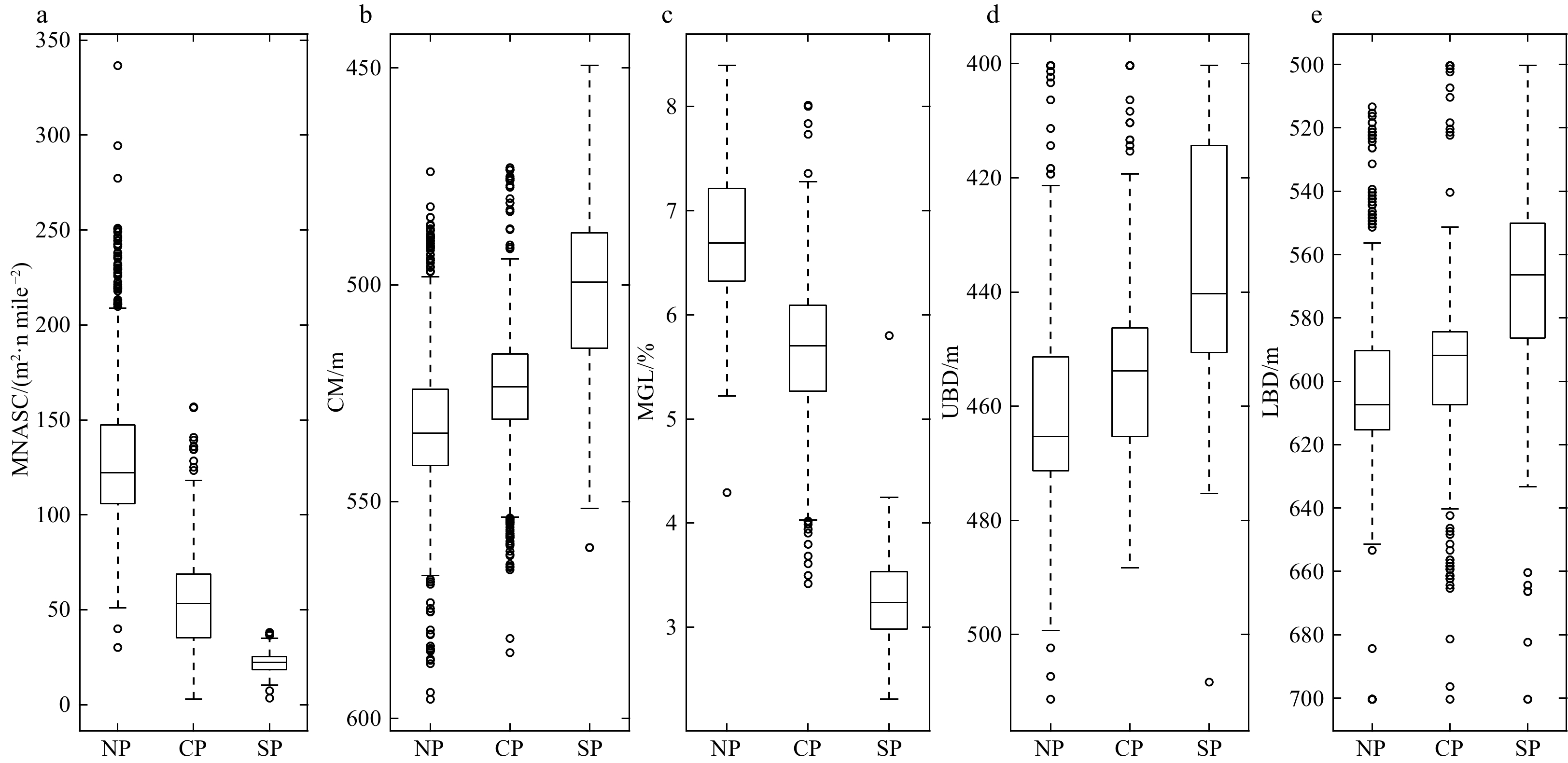
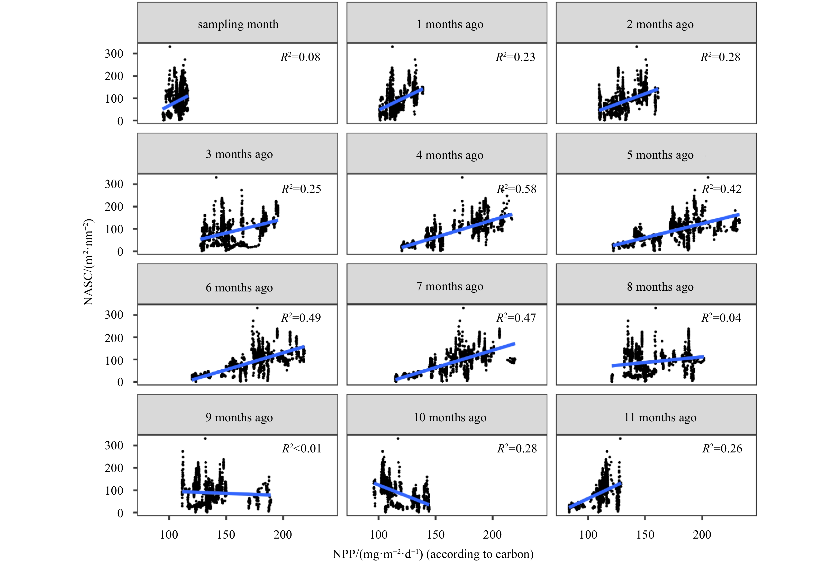
The mesopelagic communities are important for food web and carbon pump in ocean, but the large-scale studies of them are still limited until now because of the difficulties on sampling and analyzing of mesopelagic organisms. Mesopelagic organisms, especially micronekton, can form acoustic deep scattering layers (DSLs) and DSLs are widely observed. To explore the spatial patterns of DSLs and their possible influencing factors, the DSLs during daytime (10:00–14:00) were investigated in the subtropical northwestern Pacific Ocean (13°–23.5°N, 153°–163°E) using a shipboard acoustic Doppler current profiler at 38 kHz. The study area was divided into three parts using k-means cluster analysis: the northern part (NP, 22°–24°N), the central part (CP, 17°–22°N), and the southern part (SP, 12°–17°N). The characteristics of DSLs varied widely with latitudinal gradient. Deepest core DSLs (523.5 m±17.4 m), largest nautical area scattering coefficient (NASC) (130.8 m2/n mile2±41.0 m2/n mile2), and most concentrated DSLs (mesopelagic organisms gathering level, 6.7%±0.7%) were observed in NP. The proportion of migration was also stronger in NP (39.7%) than those in other parts (18.6% in CP and 21.5% in SP) for mesopelagic organisms. The latitudinal variation of DSLs was probably caused by changes in oxygen concentration and light intensity of mesopelagic zones. A positive relationship between NASC and primary productivity was identified. A four-months lag was seemed to exist. This study provides the first basin-scale baselines information of mesopelagic communities in the northwest Pacific with acoustic approach. Further researches are suggested to gain understandings of seasonal and annual variations of DSLs in the region.
Magmatism at mid-ocean ridges is one of our planet’s most important geological processes as it forms the oceanic crust, which covers nearly two-thirds of the Earth’s surface. Unlike fast spreading ridges, it is widely accepted that ultraslow–spreading ridges have relatively low extents of melting and magmatism, thinner crust, and experience limited crustal processes (Dick, 1989). Although ultraslow–spreading ridges are characterized by low magma supplies, there is also evidence of substantial magmatic processes in magma reservoirs, rather than the stable magma chambers present under some segments (Dick et al., 2003; Coogan et al., 2001; Jian et al., 2017). Until now, how magmas behave in the crust and how the thermal and dynamic regimes of the magma reservoirs and conduit systems effect the eruption mechanism of magmas from ultraslow mid-ocean ridges (MORs) has received comparatively little attention. As the product of erupted magma, mid-ocean ridge basalts (MORBs) can provide information about the magmatism under ridges (Yang et al., 2013). Therefore, unraveling the chemical effects of magmatic processes reflected by the MORBs is key to determining the details of the magma plumbing system beneath ultraslow oceanic spreading centers.
Previous studies have mainly focused on the whole–rock geochemical and isotopic compositions of MORBs from ultraslow–spreading ridges (Dick et al., 2003; Yang et al., 2013, 2017). However, whole–rock geochemistry cannot provide information about the magmatic processes occurring within the crust, which we are attempting to understand, because the bulk–rock compositions of MORBs reflect the variable overprinting of the low–pressure differentiation of mantle–derived primary liquids (Stolper, 1980; Yang et al., 2013). Unlike whole–rock compositions, the major and trace element contents of plagioclase phenocrysts are easily preserved and are sensitive to the physicochemical conditions of the melt from which they crystallized (Ginibre et al., 2004; Mollo et al., 2011; Mutch et al., 2019; Bennett et al., 2019). Their geochemical compositions and morphology are commonly used to obtain information about the conditions of the magmatic system from which they crystallized. For example, Mutch et al. (2019) established an element diffusion model for plagioclase to constrain the timescales of magmatic processes. Bennett et al. (2019) demonstrated that various plagioclase textures in mid–ocean ridge basalts can be used as indicators of various magmatic processes. In addition, the composition of plagioclase can provide information about the conditions of the magmatic system, such as the water content, temperature, and melt composition (Hellevang and Pedersen, 2008; Lange et al., 2013; Coote and Shane, 2016). These conditions are related to magma mixing, fractional crystallization, and assimilation processes. Therefore, plagioclase phenocrysts have the potential to record a magmatic history that might be obscured at the whole–rock geochemical scale. However, compared with continental and other oceanic settings, plagioclase phenocrysts are still underutilized in the study of MORBs from ultraslow spreading ridges.
In recent years, the China Ocean Mineral Resources R&D Association (COMRA) has provided support for scientific expeditions to the Southwest Indian Ridge (SWIR), during which a large number of new samples were collected (Tao et al., 2012). Among the various types of MORBs, plagioclase ultraphyric basalts (PUBs), defined by Cullen et al. (1989), are valuable due to their high plagioclase contents (10%–54%). These plagioclase phenocrysts contain unique information about crustal processes and the characteristics of the magmatic array present in the lower oceanic crust (Hellevang and Pedersen, 2008; Lange et al., 2013; Bennett et al., 2019). In this study, we examined the compositions of plagioclase phenocrysts from PUBs erupted on the SWIR (51°E), which is a typical ultraslow spreading ridge. Microanalysis of these phenocrysts provides an opportunity to investigate the geochemical changes that occurred, and thus, provides insights into the details of the magma reservoirs beneath the ultraslow oceanic spreading centers.
2.
Geologic setting
The SWIR is a typical ultraslow spreading ridge, with a half–spreading rate of around 7–9 mm/a (Dick et al., 2003). It separates the African Plate from the Antarctic Plate. The SWIR extends for 8 000 km from the Rodrigues Triple Junction (RTJ, 70°E) at its eastern end to the Bouvet Triple Junction at its western end (BTJ, 0°) (Fig. 1a). The SWIR is characterized by strong segmentation and discontinuous magmatism. Bathymetric data has revealed a shallow central region between the Prince Edward Transform Fracture Zone (35.5°E) and the Gallieni Fracture Zone (52.3°E), with an average depth of ~3 200 m compared with the deeper western (~4 000 m) and the eastern (~4 500 m) sections of the ridge (Cannat et al., 2008). As a result of the Marion hotspot to the southwest, this region has strong negative residual mantle Bouguer gravity anomalies, indicating relatively active crust–mantle exchange, deep magmatism, moderate levels of melting, and a moderate heat supply (Georgen et al., 2001; Sauter et al., 2009).
Figure
1.
Bathymetric map of the Southwest Indian Ridge (SWIR) (a) and location of the sample (b) (http://www.geomapapp.org). The location of the sample used in this study is marked by the star. BTJ: Bouvet Triple Junction; RTJ: Rodrigues Triple Junction; PE: Prince Edward Transform Fracture Zone; IFZ: Indomed Fracture Zone; GFZ: Gallieni Fracture Zone.
The study area and the sample sites are located between the Indomed (46°E) and Gallieni fracture zones (IFZ–GFZ) on the shallow central region of the SWIR (Fig. 1b). Previous geophysical and geochemical studies have been conducted on the ridge segment between the IFZ and GFZ. The center of this segment has anomalously thick crust (up to 10 km) (Niu et al., 2015) compared with that of the neighboring ridge sections. This thick oceanic crust indicates a robust magma supply in this area, which has been inferred to be associate with the Crozet hotspot (Sauter et al., 2009; Zhang et al., 2013) or with tectonic processes (Jian et al., 2017). Segments with robust magma supplies are also promising areas for hydrothermal activity (Tao et al., 2012).
3.
Sample descriptions and analytical methods
The PUB sample examined in this study was collected by television–guided grabs (TVGs) during the R/V Dayang Yihao Cruise DY115–21 to the 51°E magmatic segment in 2010. The sample was collected at a water depth of about 1 655 m. Optical microscopy analysis indicates that lavas from the SWIR are porphyritic and contain ~15% phenocrysts. The phenocrysts are mostly euhedral to subhedral plagioclase with polysynthetic twinning. The other main phase is subhedral to anhedral olivine (<1%). The plagioclase crystals contain abundant melt inclusions. The groundmass is primarily composed of suhedral, lath–like plagioclase and subordinate, anhedral olivine (Fig. 2).
Figure
2.
Photographs and representative photomicrographs (cross–polarized) of the PUB from the SWIR. a. Hand specimens of the sample; b. enhedral to subhedral plagioclase phenocrysts with melt inclusions; and c suhedral. lath–like plagioclase and subordinate, anhedral olive. Pl: plagioclase, Ol: olivine, MI: melt–melt inclusion.
Backscattered electron (BSE) imaging of the plagioclase in polished thin sections was used to characterize the textures of the crystals. Mineral analysis of the plagioclase was conducted using the JEOL JXA 8100 electron microprobe at the Key Laboratory of Submarine Geosciences (KLSG), Ministry of Natural Resources (MNR). The analytical conditions were as follows: a 15 kV accelerating voltage, a 20 nA specimen current, and a 1 μm focused beam. The peak counting times were 90 s for Fe and Mg, and 20 s for all of the other major elements. The detection limits for most of the elements, except for Ti, were lower than 400×10–6, depending on the abundance of the elements. The detection limit of Ti was 600×10–6 due to its lower content. The following natural and synthetic standards were used for the specified elements: Olivine (Si, Mg), Apatite (Ca, P), Hematite (Fe), Albite (Na, Al), Orthoclase (K), Rhodonite (Mn), Rutile (Ti), and Tugtupite (Cl). The raw data was corrected using the ZAF correction. The chemical formulas of the plagioclase phenocrysts were calculated from the mineral analysis results based on 24 anions.
4.
Results
4.1
Texture of the plagioclases
The plagioclase phenocrysts (typically >0.5 mm) from the SWIR are predominantly euhedral to subhedral in shape with tabular habits. They exhibit three textural types (Figs 3a–c). Type 1 plagioclase crystals are characterized by oscillatory zoning, surrounded by a thin rim (<50 μm). Type 2 plagioclase crystals are also characterized by oscillatory zoning, but have wider rims (50–150 μm) than Type 1 plagioclase (<50 μm). Type 3 plagioclase crystals contain numerous circular melt inclusions and do not exhibit oscillatory zoning. The plagioclase in the groundmass varies in size. The relatively large microphenocrysts typically have sizes of 0.01–0.50 mm and are primarily unzoned, whereas the relatively small groundmass microlites are <0.01 mm (Fig. 3d).
Figure
3.
Back-scattered-electron (BSE) images of the different types of plagioclase in the PUB. a. Type 1 plagioclase phenocryst; b. Type 2 plagioclase phenocryst; c. Type 3 plagioclase phenocryst; and d. plagioclase microphenocrysts. MI: melt inclusion.
A total of 25 microprobe analyses were performed on the studied sample. Representative chemical data for the plagioclases are presented in Table 1. These phenocrysts have An contents of 58 to 82. No distinct compositional differences exist among the three types of plagioclase phenocrysts. All of the phenocrysts have calcic cores (An74–82) and sodic rim growth (~An67–71). The variation from the core to the rim is 10–20 mol% An. The plagioclase crystals found within the microphenocrysts and microlites are sodic (An58–63), similar to the rims of the phenocrysts. On the ternary classification diagram, the plagioclase in the studied sample display a continuous range from bytownite to labradorite, with An decreasing from 82 to 58. The cores of the plagioclase phenocrysts are bytownite, while the rims range from bytownite to labradorite. All of the plagioclase crystals in the groundmass are labradorite with lower An contents (Fig. 4).
Table
1.
Representative microprobe data for the plagioclase from the SWIR of this study
Element
Phenocrystal
Groundmass1)
Type I
Type II
Type III
Pl-m
Pl-g
Core
Rim
Core
Rim
Core
Rim
SiO2
48.25
51.42
50.73
52.24
48.80
51.74
53.70
54.69
TiO2
0.06
0.10
0.05
0.00
0.00
0.11
0.08
0.17
Al2O3
31.49
30.03
30.28
29.61
31.70
29.81
28.41
26.72
FeO
0.29
0.40
0.50
0.54
0.38
0.62
0.58
1.41
MnO
0.04
0.00
0.04
0.00
0.00
0.00
0.00
0.00
MgO
0.15
0.19
0.24
0.18
0.20
0.20
0.18
0.37
CaO
16.80
14.52
14.94
14.01
16.29
14.13
12.77
11.92
Na2O
1.99
3.25
2.92
3.42
2.21
3.22
4.15
4.64
K2O
0.01
0.02
0.01
0.03
0.01
0.02
0.04
0.06
P2O5
0.01
0.03
0.00
0.02
0.01
0.00
0.01
0.05
Total
99.08
99.95
99.71
100.04
99.59
99.86
99.92
100.02
Calculated atoms based on 24 oxygens
Si
6.704
7.031
6.962
7.127
6.736
7.072
7.311
7.457
Ti
0.006
0.010
0.005
0.000
0.000
0.011
0.008
0.017
Al
5.157
4.840
4.899
4.761
5.157
4.803
4.559
4.294
Fe
0.034
0.046
0.057
0.062
0.043
0.071
0.066
0.161
Mn
0.005
0.000
0.004
0.000
0.000
0.000
0.000
0.000
Mg
0.031
0.039
0.049
0.036
0.041
0.041
0.037
0.074
Ca
2.501
2.127
2.198
2.047
2.409
2.070
1.863
1.742
Na
0.536
0.862
0.776
0.905
0.591
0.852
1.096
1.225
K
0.002
0.003
0.002
0.005
0.001
0.003
0.007
0.011
P
0.002
0.003
0.000
0.002
0.001
0.000
0.001
0.005
Total
14.977
14.961
14.953
14.945
14.980
14.924
14.947
14.987
An
0.82
0.71
0.74
0.69
0.80
0.71
0.63
0.58
Ab
0.18
0.29
0.26
0.31
0.20
0.29
0.37
0.41
Or
0.00
0.00
0.00
0.00
0.00
0.00
0.00
0.01
FeO/MgO
1.91
2.12
2.08
3.04
1.90
3.06
3.16
3.87
Ca/Na
4.67
2.47
2.83
2.26
4.07
2.43
1.70
1.42
T/°C2)
1296
1108
1237
1098
1280
1129
1063
1042
Note: 1) Pl-m and Pl-g represent plagioclase microphenocrysts and microlites in groundmass, respectively; 2) crystallization temperature is calculated according to Kudo and Weill (1983).
In terms of the major elements, the FeO and MgO concentrations of the plagioclase do not vary significantly. The FeO and MgO concentrations are 0.29%–1.41% (wt) and 0.15%–0.37% (wt), respectively. The FeO and MgO concentrations of the plagioclase cores are relatively depleted compared with those of the plagioclase rims and groundmass.
5.
Discussion
5.1
Crystallization temperature
Plagioclase compositions are a useful indicator of crystallization temperature (Kudo and Weill, 1970; Mollo et al., 2011). In this study, the plagioclase–melt geothermometry method proposed by Kudo and Weill (1970) was used to estimate the crystallization temperature of the plagioclase. Before applying the geothermometry method, the pressures must be determined. According to Chen et al. (2002), the pressures of the plagioclase rims and cores are approximately 0.5×10⁸ and 1.0×10⁸ Pa, respectively. Similarly, the plagioclase in the groundmass is estimated to have crystallized at shallower depths, within the upper crust or on the seabed. The pressure of the groundmass is also assumed to be 0.5×10⁸ Pa according to Chen et al. (2002). Based on the assumptions stated above, Eqs (1) and (2) were used to calculate the crystallization temperatures of the plagioclase crystals:
where $ \lambda$=(XNaXSi/XCaXAl) is for the groundmass, $ \sigma$=(XAbγAb/XAnγAn) is for the plagioclase, and $ \varphi$=(XCa+XAl–XSi–XNa) is for the groundmass. X represents the mole fraction of the component. Although the groundmass is microcrystalline and lacks glass, Lange et al. (2013) demonstrated that PUB hosted glasses have the same range of compositions as aphyric lavas from the same segment. Therefore, in the calculation process, we use the average whole–rock compositions of the aphyric basalts from the same segment, which were reported by Yang et al. (2014), as an approximate proxy for the groundmass.
According to the plagioclase geothermometer described above, the crystallization temperatures of the phenocryst cores and rims are (1 273±18)°C and (1 099±10)°C, respectively. From the core to the rim of the phenocryst, the crystallization temperature decreases by about 200°C. The crystallization temperatures of the microphenocrysts and microlites in the groundmass range from 1 063°C to 1 087°C (average = 1 072°C), which is similar to the crystallization temperature of the phenocryst rims (Table 1).
In previous studies, the crystallization temperatures of high–An (An≥70%) plagioclase phenocrysts, which were estimated from the entrapment temperature of melt inclusions in samples from ultraslow spreading ridges, were found to range from 1 230°C to 1 260°C (Nielsen et al., 1995; Drignon et al., 2019). Whereas the minimum estimation of the crystallization temperature of low An (An<70%) plagioclase is 1 100°C (Yang et al., 2019). The crystallization temperatures in our study are consistent with these results, which suggests that our calculated results are reasonable and the plagioclases thermometer by Kudo and Weill (1970) can be used to calculate the crystallization temperatures of plagioclase phenocrysts from MORBs beneath ultraslow ridges.
5.2
Plagioclase–melt equilibrium
5.2.1
Major elements
In plagioclase, the diffusion rates of major elements, such as the NaSi–CaAl exchange, are extremely slow (Grove et al., 1984). The geochemical zoning of the crystals likely reflects the magmatic conditions, and thus, it can be used to investigate the likelihood of plagioclase–melt equilibrium. Previous experiments have demonstrated that the partition coefficient of Ca/Na (KCa/Na) between plagioclase and melt mainly positively depends on the water content of the magma (Sisson and Grove, 1993; Martel et al., 2006). For basaltic magmas from mid-ocean ridges, when the magmatic water content is 3%, KCa/Na is typically ~1 for mid to upper lithospheric pressures (<10×108 Pa) (Sisson and Grove, 1993). The magmatic water contents of the SWIR lavas are close to the global average value for the upper mantle (0.3%–0.4%) (Robinson et al., 2001), which indicates that their KCa/Na value is less than 1.
In addition to the KCa/Na value, a representative melt composition is required to assess the equilibrium composition of the plagioclase phenocrysts. The groundmass of these rocks is microcrystalline and lacks glass, so it represents the final melt. Thus, as was discussed above, the average whole–rock composition of the aphyric basalts from the same segment is representative of the groundmass composition. The reported composition of the basalts and glass from this ridge segment do not vary significantly, with molar Ca/Na values ranging from 2.11 to 2.68 (Yang et al., 2014; Bézos and Humler, 2005). The molar Ca/Na values of the plagioclase phenocrysts in equilibrium with the melt are consistently≤2.68 (Fig. 5). The molar Ca/Na values of the plagioclase rims and groundmass range from 1.42 to 2.47, which is in equilibrium with the melt (Fig. 5). However, the compositions of the plagioclase cores (Ca/Na = 3 to 4) are higher than the upper limit of the equilibrium melt (Ca/Na = 2.68) (Fig. 5). In addition, the crystallization temperatures of the plagioclase cores (average of 1 273°C) are close to the experimental melting point of basaltic magma (~1 300°C) and the estimated upper mantle potential temperature of the SWIR lavas (~1 280°C) (Kamenetsky et al., 2000; Robinson et al., 2001). Therefore, the plagioclase cores are unlikely to have formed in the host magma. Instead, they are most likely xenocrysts, which crystallized from a more calcic melt.
Figure
5.
Ca/Na molecular ratio of the plagioclase compared with that of the melt. The melt represents the range of glass and whole-rock compositions, the data are obtained from Yang et al. (2014) and Bézos and Humler (2005). The K values and water contents are from Martel et al. (2006). Equilibrium between the plagioclase and melts is possible in the shaded area.
It is worth noting that compared with the plagioclase rims, the plagioclase phenocrysts in the groundmass have lower Ca/Na ratios (<2). Their more sodic compositions are most likely due to decreasing magmatic water contents caused by the fact that the KCa/Na between the plagioclase and the melt decreases as of the water content of the magma increases (Martel and Schmidt, 2003). Water is lost during the late-stage of magma ascent through the conduit due to ascent–driven decompression of the water-saturated magma. Thus, the compositional variations can be explained by the variations in the magmatic water content.
5.2.2
Mg and Fe contents of the plagioclase
The MgO zoning patterns of the plagioclase phenocrysts have the potential to record the magmatic composition because the Mg contents of the plagioclase phenocrysts reflect the composition of the host melt (Ginibre et al., 2002). Although it is difficult to accurately estimate the Mg partition coefficient (KMg) between plagioclase and melt, empirical studies have suggested an Arrhenius-like relationship of decreasing KMg with increasing XAn (Bindeman et al., 1998). To investigate the equilibrium relationship between the SWIR plagioclase and the host magma, we estimated the KMg based on this empirical relationship, which is often used to determine whether plagioclase phenocrysts are in equilibrium with the melt in magmatic systems (Bindeman et al., 1998; Coote and Shane, 2016). The majority of the plagioclase phenocrysts analyzed in this study are more enriched in MgO than the modeled melt compositions for a crystallization temperature of ~1099°C, which is based on the plagioclase geothermometer described above (Fig. 6a). This implies that the plagioclase in the PUBs analyzed in this study could not have crystallized from the basaltic host melt (MgO of 6.38%–8.87% (wt), average of 7.77% (wt)) and would require a more mafic melt (MgO of up to 14% (wt)). This agrees with the major element modeling (Ca/Na) of the plagioclase cores, but does not agree with the equilibrium between the rims and the melt suggested by the Ca/Na ratios (Fig. 5).
Figure
6.
Compositional plots of An versus MgO (a) and FeO/MgO (b) for the plagioclase. The curves represent plagioclase equilibrium compositions based on the KMg values from Bindeman et al. (1998) and a temperature of 1099℃ obtained from the plagioclase geothermometer. The average crystallization temperature of the phenocryst rims is 1099°C. The following melt parameters were used: (1) MgO=14%, the upper limit of the MgO content of the matrix melt according to a simulation based on the model of Bindeman et al. (1998); (2) MgO=7.77%, the average whole-rock composition of the aphyric basalts in the same segment from the literature, which is representative of the matrix.
The rimward increase in Mg and decrease in An appear to be similar to the trends described in previous diffusion studies (Costa et al., 2003; Moore et al., 2014). When minerals crystallize due to large degrees of undercooling and the diffusion in the melt cannot keep pace with the crystal formation, it is possible for late–stage rapid disequilibrium crystallization to produce a boundary layer melt enriched in incompatible (Fe, Mg) elements (Ginibre et al., 2002; Coote et al., 2018). This could explain the elevated MgO contents of the plagioclase rims and the groundmass plagioclase relative to the equilibrium values (Fig. 6a). The internal disequilibrium in the MgO contents can be explained by the mixing of primitive (MgO=14% (wt)) and more evolved magmas (MgO=7.77%(wt)).
Additionally, in plagioclase, the post–crystallization diffusion of Fe is slower than that of Mg (Costa et al., 2003). Thus, the highest FeO/MgO ratios occur in the outermost parts of the rims and in the groundmass plagioclase (Fig. 6b) due to the fact that FeO diffuses into the plagioclase more slowly than MgO, and thus, more FeO accumulates in the boundary layer during a short residence time. However, it is worth noting that since the FeO content of the plagioclase depends on both the melt composition and the oxygen fugacity, it is difficult to assess the plagioclase–melt equilibrium using only the FeO content (Coote et al., 2018). Therefore, disequilibrium diffusion within a short time period can result in elevated Mg contents compared with the equilibrium values and the highest FeO/MgO ratios occurring in the plagioclase rims (Coote and Shane, 2016; Moore et al., 2014). Whereas the discrepancies in the plagioclase–melt equilibrium inferred from the major elements (Ca/Na) and the Mg contents are likely an artifact of disequilibrium diffusion (Coote and Shane, 2016).
5.3
Implications for the SWIR magma system
In the SWIR, the crystallization temperature and composition of the plagioclase cores are distinctly different from those of the rims (Table 1), which indicates that the plagioclase cores and rims have different thermal histories.
The plagioclase cores are usually uniform and exhibit oscillatory zoning. The oscillatory zoning results in small-scale compositional variations, which suggests a regime of near–constant intensive parameters (pressure, temperature) (Landi et al., 2004; Shcherbakov et al., 2011). These characteristics suggest the cores crystallized from a stable environment and do not have complex crystallization histories. Besides, the presence of cores in plagioclase that are too primitive to be in equilibrium with the host magma indicates that they crystallized from a more primitive region in the plumbing system and were picked up by a more evolved melt later. Thus, we propose that the plagioclase cores grew in a stable mush zone where the temperature was high and constant, and were later entrained into a more evolved melt.
The thin plagioclase rims (normally < 150 μm) have lower crystallization temperatures and lower An values than the cores, and their major elements (Ca/Na) are in equilibrium with the host magma. These characteristics demonstrate that they crystallized from the host melt, which is more evolved than the magma from which the cores crystalized. Similarly, the plagioclase microphenocrysts and microlites are also in equilibrium (Ca/Na) values with the host magma, which suggests that they crystallized from the host magma as well. Compared with fast to intermediate spreading ridges, there are generally no stable magma chambers and the volume of melt may be low under ultraslow mid–ocean ridges (Dick et al., 2003). Thus, the transport of magma into cooler regions of the reservoir would be expected to result in abrupt, strong undercooling of the magma. Due to these large degrees of rapid cooling, the plagioclase phenocrysts in SWIR PUBs generally have thin rims. The plagioclase rims of the phenocrysts exhibit major element (Fe, Mg) enrichment because these elements cannot reach equilibrium when diffusing from the host magma into the plagioclase phenocrysts. The MgO contents of the outermost rims of the plagioclase can be used to calculate the maximum time between the incorporation of the plagioclase into the host melt and quenching on the seafloor (Costa et al., 2003; Moore et al., 2014). We used Eq. (8) in Costa et al. (2003) to determine the Mg diffusion coefficient of the plagioclase. The maximum residence time of the plagioclases in the host melt was nearly 5–8 d. The close temporal relationship between the evolved magma replenishment and the eruption suggests that replenishment plays an important role in driving the eruption, which has also been suggested for other MORB eruptions on slow and intermediate ridges (Costa et al., 2010). Overall, our favored model is that replenishment by an evolved melt under the SWIR ridges (51°E) drives the eruption over a short period of time.
6.
Conclusions
(1) The plagioclase cores with high An values have higher crystallization temperatures (1 273±18)°C than the rims (1 099±10)°C. The range of crystallization temperatures for the microphenocrysts and microlites in the groundmass is similar to that of the phenocryst rims.
(2) The compositions of the plagioclase cores from the SWIR indicate that they did not form in the host magma, but xenocrysts are crystallized from a more mafic melt composition. Whereas the plagioclase rims and the microphenocrysts and microlites in the groundmass are in equilibrium with the host basaltic melts.
(3) The disequilibrium MgO contents and the higher FeO/MgO ratios of the rims of the plagioclase phenocrysts reflect shorter magmatic residence time periods than would be resulting from equilibrium diffusion.
(4) An evolved melt replenished the magma under the SWIR ridges (51°E), driving the eruption over a short period of time.
Acknowledgements
We are grateful to Yin-Jia Jin and two anonymous reviewers for their careful editing and constructive comments, which improved the manuscript. We also thank the crew and scientists involved in the R/V Dayang Yihao Cruise DY115–21.
Aksnes D L, Røstad A, Kaartvedt S, et al. 2017. Light penetration structures the deep acoustic scattering layers in the global ocean. Science Advances, 3(5): e1602468. doi: 10.1126/sciadv.1602468
[2]
Ariza A, Garijo J C, Landeira J M, et al. 2015. Migrant biomass and respiratory carbon flux by zooplankton and micronekton in the subtropical Northeast Atlantic Ocean (Canary Islands). Progress in Oceanography, 134: 330–342. doi: 10.1016/j.pocean.2015.03.003
[3]
Béhagle N, Cotté C, Lebourges-Dhaussy A, et al. 2017. Acoustic distribution of discriminated micronektonic organisms from a bi-frequency processing: the case study of eastern Kerguelen oceanic waters. Progress in Oceanography, 156: 276–289. doi: 10.1016/j.pocean.2017.06.004
[4]
Béhagle N, Cotté C, Ryan T E, et al. 2016. Acoustic micronektonic distribution is structured by macroscale oceanographic processes across 20–50°S latitudes in the South-Western Indian Ocean. Deep-Sea Research Part I: Oceanographic Research Papers, 110: 20–32. doi: 10.1016/j.dsr.2015.12.007
[5]
Benoit-Bird K J, Lawson G L. 2016. Ecological insights from pelagic habitats acquired using active acoustic techniques. Annual Review of Marine Science, 8(1): 463–490. doi: 10.1146/annurev-marine-122414-034001
[6]
Bertrand A, Ballón M, Chaigneau A. 2010. Acoustic observation of living organisms reveals the upper limit of the oxygen minimum zone. PLoS ONE, 5(4): e10330. doi: 10.1371/journal.pone.0010330
[7]
Bertrand A, Bard F X, Josse E. 2002. Tuna food habits related to the micronekton distribution in French Polynesia. Marine Biology, 140(5): 1023–1037. doi: 10.1007/s00227-001-0776-3
[8]
Bianchi D, Galbraith E D, Carozza D A, et al. 2013. Intensification of open-ocean oxygen depletion by vertically migrating animals. Nature Geoscience, 6(7): 545–548. doi: 10.1038/ngeo1837
[9]
Bianchi D, Mislan K A S. 2016. Global patterns of diel vertical migration times and velocities from acoustic data. Limnology and Oceanography, 61(1): 353–364. doi: 10.1002/lno.10219
[10]
Boswell K M, D’Elia M, Johnston M W, et al. 2020. Oceanographic structure and light levels drive patterns of sound scattering layers in a low-latitude oceanic system. Frontiers in Marine Science, 7: 51. doi: 10.3389/fmars.2020.00051
[11]
Brierley A S. 2014. Diel vertical migration. Current Biology, 24(22): R1074–R1076. doi: 10.1016/j.cub.2014.08.054
[12]
Carr M E, Friedrichs M A M, Schmeltz M, et al. 2006. A comparison of global estimates of marine primary production from ocean color. Deep-Sea Research Part II: Topical Studies in Oceanography, 53(5−7): 741–770. doi: 10.1016/j.dsr2.2006.01.028
[13]
Cascão I, Domokos R, Lammers M O, et al. 2019. Seamount effects on the diel vertical migration and spatial structure of micronekton. Progress in Oceanography, 175: 1–13. doi: 10.1016/j.pocean.2019.03.008
[14]
Catul V, Gauns M, Karuppasamy P K. 2011. A review on mesopelagic fishes belonging to family Myctophidae. Reviews in Fish Biology and Fisheries, 21(3): 339–354. doi: 10.1007/s11160-010-9176-4
[15]
Cayre P. 1991. Behaviour of yellowfin tuna (Thunnus albacares) and skipjack tuna (Katsuwonus pelarnis) around fish aggregating devices (FADs) in the Comoros Islands as determined by ultrasonic tagging. Aquatic Living Resources, 4(1): 1–12. doi: 10.1051/alr/1991000
[16]
Chikuni S. 1985. The fish resources of the Northwest Pacific. Rome: FAO
[17]
Christiansen B, Denda A, Christiansen S. 2020. Potential effects of deep seabed mining on pelagic and benthopelagic biota. Marine Policy, 114: 103442. doi: 10.1016/j.marpol.2019.02.014
[18]
Condie S A, Dunn J R. 2006. Seasonal characteristics of the surface mixed layer in the Australasian region: implications for primary production regimes and biogeography. Marine and Freshwater Research, 57(6): 569–590. doi: 10.1071/MF06009
[19]
Coull J R. 1993. World Fisheries Resources. New York: Routledge, 6–18
[20]
Deines K L. 1999. Backscatter estimation using broadband acoustic Doppler current profilers. In: Proceedings of the IEEE Sixth Working Conference on Current Measurement. San Diego, CA: IEEE, 249–253
[21]
Diogoul N, Brehmer P, Perrot Y, et al. 2020. Fine-scale vertical structure of sound-scattering layers over an east border upwelling system and its relationship to pelagic habitat characteristics. Ocean Science, 16(1): 65–81. doi: 10.5194/os-16-65-2020
[22]
Escobar-Flores P, O’Driscoll R L, Montgomery J C. 2013. Acoustic characterization of pelagic fish distribution across the South Pacific Ocean. Marine Ecology Progress Series, 490: 169–183. doi: 10.3354/meps10435
[23]
Escobar-Flores P, O’Driscoll R L, Montgomery J C. 2018. Spatial and temporal distribution patterns of acoustic backscatter in the New Zealand sector of the Southern Ocean. Marine Ecology Progress Series, 592: 19–35. doi: 10.3354/meps12489
[24]
Everitt B S, Skrondal A. 1998. The Cambridge Dictionary of Statistics. Cambridge: Cambridge University Press, 89
[25]
FAO. 2018. The state of world fisheries and aquaculture. Rome: FAO
[26]
Fennell S, Rose G. 2015. Oceanographic influences on Deep Scattering Layers across the North Atlantic. Deep-Sea Research Part I: Oceanographic Research Papers, 105: 132–141. doi: 10.1016/j.dsr.2015.09.002
[27]
Gjøsaeter J, Kawaguchi K. 1980. A review of the world resources of mesopelagic fish. Rome: FAO
[28]
Godø O R, Samuelsen A, Macaulay G J, et al. 2012. Mesoscale eddies are oases for higher trophic marine life. PLoS ONE, 7(1): e30161. doi: 10.1371/journal.pone.0030161
[29]
Gorelova T A. 1984. A quantitative assessment of consumption of zooplankton by epipelagic lanternfishes (family Myctophidae) in the equatorial Pacific Ocean. Journal of Ichthyology, 23: 106–113
[30]
Grabowski E, Letelier R M, Laws E A, et al. 2019. Coupling carbon and energy fluxes in the North Pacific Subtropical Gyre. Nature Communications, 10: 1895. doi: 10.1038/s41467-019-09772-z
[31]
Hernández-León S, Koppelmann R, Fraile-Nuez E, et al. 2020. Large deep-sea zooplankton biomass mirrors primary production in the global ocean. Nature Communications, 11(1): 6048. doi: 10.1038/s41467-020-19875-7
[32]
Hu Dunxin, Wu Lixin, Cai Wenju, et al. 2015. Pacific western boundary currents and their roles in climate. Nature, 522(7556): 299–308. doi: 10.1038/nature14504
[33]
Ingham M C, Cook S K, Hausknecht K A. 1977. Oxycline characteristics and skipjack tuna distribution in the southeastern tropical Atlantic. Fishery Bulletin, 75(4): 857–865
[34]
Inoue R, Kitamura M, Fujiki T. 2016. Diel vertical migration of zooplankton at the S1 biogeochemical mooring revealed from acoustic backscattering strength. Journal of Geophysical Research:Oceans, 121(2): 1031–1050. doi: 10.1002/2015JC011352
[35]
Irigoien X, Klevjer T A, Røstad A, et al. 2014. Large mesopelagic fishes biomass and trophic efficiency in the open ocean. Nature Communications, 5: 3271. doi: 10.1038/ncomms4271
[36]
Jennings S, Mélin F, Blanchard J L, et al. 2008. Global-scale predictions of community and ecosystem properties from simple ecological theory. Proceedings of the Royal Society B: Biological Sciences, 275(1641): 1375–1383. doi: 10.1098/rspb.2008.0192
[37]
Karl D M, Bidigare R R, Letelier R M. 2001. Long-term changes in plankton community structure and productivity in the North Pacific Subtropical Gyre: The domain shift hypothesis. Deep-Sea Research Part II: Topical Studies in Oceanography, 48(8−9): 1449–1470. doi: 10.1016/S0967-0645(00)00149-1
[38]
Keeling R F, Körtzinger A, Gruber N. 2010. Ocean deoxygenation in a warming world. Annual Review of Marine Science, 2: 199–229. doi: 10.1146/annurev.marine.010908.163855
[39]
Klevjer T A, Irigoien X, Røstad A, et al. 2016. Large scale patterns in vertical distribution and behaviour of mesopelagic scattering layers. Scientific Reports, 6: 19873. doi: 10.1038/srep19873
[40]
Klevjer T, Melle W, Knutsen T, et al. 2020. Micronekton biomass distribution, improved estimates across four north Atlantic basins. Deep-Sea Research Part II: Topical Studies in Oceanography, 180: 104691. doi: 10.1016/j.dsr2.2019.104691
[41]
Kloser R J, Ryan T E, Young J W, et al. 2009. Acoustic observations of micronekton fish on the scale of an ocean basin: potential and challenges. ICES Journal of Marine Science, 66(6): 998–1006. doi: 10.1093/icesjms/fsp077
[42]
Kwong L E, Henschke N, Pakhomov E A, et al. 2020. Mesozooplankton and micronekton active carbon transport in contrasting eddies. Frontiers in Marine Science, 6: 825. doi: 10.3389/fmars.2019.00825
Lindstrom M J, Bates D M. 1988. Newton-raphson and EM algorithms for linear mixed-effects models for repeated-measures data. Journal of the American Statistical Association, 83(404): 1014–1022
[45]
Lindstrom E, Lukas R, Fine R, et al. 1987. The western equatorial Pacific Ocean circulation study. Nature, 330(6148): 533–537. doi: 10.1038/330533a0
[46]
Liu H, Nolla H A, Campbell L. 1997. Prochlorococcus growth rate and contribution to primary production in the equatorial and subtropical North Pacific Ocean. Aquatic Microbial Ecology, 12(1): 39–47
[47]
Longhurst A R. 2007. Ecological Geography of the Sea. 2nd ed. London: Academic Press, 327–385
[48]
Longhurst A R, Glen Harrison W. 1989. The biological pump: profiles of plankton production and consumption in the upper ocean. Progress in Oceanography, 22(1): 47–123. doi: 10.1016/0079-6611(89)90010-4
[49]
MacLennan D N, Fernandes P G, Dalen J. 2002. A consistent approach to definitions and symbols in fisheries acoustics. ICES Journal of Marine Science, 59(2): 365–369. doi: 10.1006/jmsc.2001.1158
[50]
McKelvie D S. 1989. Latitudinal variation in aspects of the biology of Cyclothone braueri and C. microdon (Pisces: Gonostomatidae) in the eastern North Atlantic Ocean. Marine Biology, 102(3): 413–424. doi: 10.1007/BF00428494
[51]
Miller K A, Thompson K F, Johnston P, et al. 2018. An overview of seabed mining including the current state of development, environmental impacts, and knowledge gaps. Frontiers in Marine Science, 4: 418. doi: 10.3389/fmars.2017.00418
[52]
Moline M A, Benoit-Bird K, O’Gorman D, et al. 2015. Integration of scientific echo sounders with an adaptable autonomous vehicle to extend our understanding of animals from the surface to the bathypelagic. Journal of Atmospheric and Oceanic Technology, 32(11): 2173–2186. doi: 10.1175/JTECH-D-15-0035.1
[53]
Mote P W, Salathé E P. 2010. Future climate in the Pacific Northwest. Climatic Change, 102(1−2): 29–50. doi: 10.1007/s10584-010-9848-z
[54]
Mullison J. 2017. Backscatter estimation using broadband acoustic Doppler current profilers-updated. In: Hydraulic Measurements & Experimental Methods Conference. Durham, NH: ASCE
[55]
Netburn A N, Anthony Koslow J. 2015. Dissolved oxygen as a constraint on daytime deep scattering layer depth in the southern California current ecosystem. Deep-Sea Research Part I: Oceanographic Research Papers, 104: 149–158. doi: 10.1016/j.dsr.2015.06.006
[56]
Oestreich W K, Ganju N K, Pohlman J W, et al. 2016. Colored dissolved organic matter in shallow estuaries: relationships between carbon sources and light attenuation. Biogeosciences, 13(2): 583–595. doi: 10.5194/bg-13-583-2016
[57]
Padial A A, Thomaz S M. 2008. Prediction of the light attenuation coefficient through the Secchi disk depth: empirical modeling in two large Neotropical ecosystems. Limnology, 9(2): 143–151. doi: 10.1007/s10201-008-0246-4
[58]
Pakhomov E A, Podeswa Y, Hunt B P V, et al. 2019. Vertical distribution and active carbon transport by pelagic decapods in the North Pacific Subtropical Gyre. ICES Journal of Marine Science, 76(3): 702–717. doi: 10.1093/icesjms/fsy134
[59]
Phillips A J, Brodeur R D, Suntsov A V. 2009. Micronekton community structure in the epipelagic zone of the northern California Current upwelling system. Progress in Oceanography, 80(1−2): 74–92. doi: 10.1016/j.pocean.2008.12.001
[60]
Polis G A, Anderson W B, Holt R D. 1997. Toward an integration of landscape and food web ecology: the dynamics of spatially subsidized food webs. Annual Review of Ecology and Systematics, 28(1): 289–316. doi: 10.1146/annurev.ecolsys.28.1.289
[61]
Prince E D, Goodyear C P. 2006. Hypoxia-based habitat compression of tropical pelagic fishes. Fisheries Oceanography, 15(6): 451–464. doi: 10.1111/j.1365-2419.2005.00393.x
[62]
Proud R, Cox M J, Brierley A S. 2017. Biogeography of the global ocean’s mesopelagic zone. Current Biology, 27(1): 113–119. doi: 10.1016/j.cub.2016.11.003
[63]
Receveur A, Kestenare E, Allain V, et al. 2020. Micronekton distribution in the Southwest Pacific (New Caledonia) inferred from shipboard-ADCP backscatter data. Deep-Sea Research Part I: Oceanographic Research Papers, 159: 103237. doi: 10.1016/j.dsr.2020.103237
[64]
Salvanes A G V, Kristoffersen J B. 2001. Mesopelagic fishes. In: Steel J, Thorpe S, Turekian K, eds. Encyclopedia of Ocean Sciences. San Diego: Academic Press, 1711–1717
[65]
Sato M, Benoit-Bird K J. 2017. Spatial variability of deep scattering layers shapes the Bahamian mesopelagic ecosystem. Marine Ecology Progress Series, 580: 69–82. doi: 10.3354/meps12295
[66]
Seibel B A. 2011. Critical oxygen levels and metabolic suppression in oceanic oxygen minimum zones. Journal of Experimental Biology, 214(2): 326–336. doi: 10.1242/jeb.049171
[67]
Shen G, Shi B. 2002. Primary Production in Marine. Beijing: Science Press, 189–223
[68]
Sibson R. 1981. A brief description of natural neighbor interpolation. In: Barnett V, ed. Interpreting Multivariate Data. New York: John Wiley & Sons, 21–36
[69]
Smeti H, Pagano M, Menkes C, et al. 2015. Spatial and temporal variability of zooplankton off New Caledonia (Southwestern Pacific) from acoustics and net measurements. Journal of Geophysical Research: Oceans, 120(4): 2676–2700. doi: 10.1002/2014JC010441
[70]
St John M A, Borja A, Chust G, et al. 2016. A dark hole in our understanding of marine ecosystems and their services: Perspectives from the mesopelagic community. Frontiers in Marine Science, 3: 31
[71]
Stedmon C A, Nelson N B. 2015. The optical properties of DOM in the ocean. In: Hansell D A, Carlson C A, eds. Biogeochemistry of Marine Dissolved Organic Matter. 2nd ed. San Diego: Academic Press, 481–508
[72]
Steinacher M, Joos F, Frölicher T L, et al. 2010. Projected 21st century decrease in marine productivity: a multi-model analysis. Biogeosciences, 7(3): 979–1005. doi: 10.5194/bg-7-979-2010
[73]
Steinberg D K, Cope J S, Wilson S E, et al. 2008a. A comparison of mesopelagic mesozooplankton community structure in the subtropical and subarctic North Pacific Ocean. Deep-Sea Research Part II: Topical Studies in Oceanography, 55(14−15): 1615–1635. doi: 10.1016/j.dsr2.2008.04.025
[74]
Steinberg D K, Van Mooy B A S, Buesseler K O, et al. 2008b. Bacterial vs. zooplankton control of sinking particle flux in the ocean’s twilight zone. Limnology and Oceanography, 53(4): 1327–1338. doi: 10.4319/lo.2008.53.4.1327
[75]
Stramma L, Prince E D, Schmidtko S, et al. 2012. Expansion of oxygen minimum zones may reduce available habitat for tropical pelagic fishes. Nature Climate Change, 2(1): 33–37. doi: 10.1038/nclimate1304
[76]
Toole J M, Zou E, Millard R C. 1988. On the circulation of the upper waters in the western equatorial Pacific Ocean. Deep-Sea Research Part A. Oceanographic Research Papers, 35(9): 1451–1482
[77]
Urmy S S, Horne J K. 2016. Multi-scale responses of scattering layers to environmental variability in Monterey Bay, California. Deep-Sea Research Part I: Oceanographic Research Papers, 113: 22–32. doi: 10.1016/j.dsr.2016.04.004
[78]
Urmy S S, Horne J K, Barbee D H. 2012. Measuring the vertical distributional variability of pelagic fauna in Monterey Bay. ICES Journal of Marine Science, 69(2): 184–196. doi: 10.1093/icesjms/fsr205
[79]
Zhang Dongsheng, Wang Chunsheng, Liu Zhensheng, et al. 2012. Spatial and temporal variability and size fractionation of chlorophyll a in the tropical and subtropical Pacific Ocean. Acta Oceanologica Sinica, 31(3): 120–131. doi: 10.1007/s13131-012-0212-1
Marian Peña. Atlantic versus Mediterranean deep scattering layers around the Iberian peninsula. Progress in Oceanography, 2024, 221: 103211. doi:10.1016/j.pocean.2024.103211
2.
Zhenhong Zhu, Jianfeng Tong, Minghua Xue, et al. Assessing the influence of abiotic factors on small pelagic fish distribution across diverse water layers in the Northwest Pacific Ocean through acoustic methods. Ecological Indicators, 2024, 158: 111563. doi:10.1016/j.ecolind.2024.111563
3.
Zixuan Niu, Zhaohui Chen, Wei Yu, et al. Temporal and spatial variations in squid jigging catch efficiency in the Oyashio Extension region. Fisheries Oceanography, 2024. doi:10.1111/fog.12692
4.
Réka Domokos. Spatiotemporal variability of micronekton at two central North Pacific Fronts. Deep Sea Research Part I: Oceanographic Research Papers, 2023, 198: 104076. doi:10.1016/j.dsr.2023.104076
5.
Lingyun Nie, Jianchao Li, Hao Wu, et al. The Influence of Ocean Processes on Fine-Scale Changes in the Yellow Sea Cold Water Mass Boundary Area Structure Based on Acoustic Observations. Remote Sensing, 2023, 15(17): 4272. doi:10.3390/rs15174272
ZHU Yanbing, LI Hebin, NI Hui, LIU Jingwen, XIAO Anfeng, CAI Huinong. Purification and biochemical characterization of manganesecontaining superoxide dismutase from deep-sea thermophile Geobacillus sp. EPT3[J]. Acta Oceanologica Sinica, 2014, 33(12): 163-169. doi: 10.1007/s13131-014-0534-2
ZHU Yanbing, LI Hebin, NI Hui, LIU Jingwen, XIAO Anfeng, CAI Huinong. Purification and biochemical characterization of manganesecontaining superoxide dismutase from deep-sea thermophile Geobacillus sp. EPT3[J]. Acta Oceanologica Sinica, 2014, 33(12): 163-169. doi: 10.1007/s13131-014-0534-2
Table
1.
Representative microprobe data for the plagioclase from the SWIR of this study
Element
Phenocrystal
Groundmass1)
Type I
Type II
Type III
Pl-m
Pl-g
Core
Rim
Core
Rim
Core
Rim
SiO2
48.25
51.42
50.73
52.24
48.80
51.74
53.70
54.69
TiO2
0.06
0.10
0.05
0.00
0.00
0.11
0.08
0.17
Al2O3
31.49
30.03
30.28
29.61
31.70
29.81
28.41
26.72
FeO
0.29
0.40
0.50
0.54
0.38
0.62
0.58
1.41
MnO
0.04
0.00
0.04
0.00
0.00
0.00
0.00
0.00
MgO
0.15
0.19
0.24
0.18
0.20
0.20
0.18
0.37
CaO
16.80
14.52
14.94
14.01
16.29
14.13
12.77
11.92
Na2O
1.99
3.25
2.92
3.42
2.21
3.22
4.15
4.64
K2O
0.01
0.02
0.01
0.03
0.01
0.02
0.04
0.06
P2O5
0.01
0.03
0.00
0.02
0.01
0.00
0.01
0.05
Total
99.08
99.95
99.71
100.04
99.59
99.86
99.92
100.02
Calculated atoms based on 24 oxygens
Si
6.704
7.031
6.962
7.127
6.736
7.072
7.311
7.457
Ti
0.006
0.010
0.005
0.000
0.000
0.011
0.008
0.017
Al
5.157
4.840
4.899
4.761
5.157
4.803
4.559
4.294
Fe
0.034
0.046
0.057
0.062
0.043
0.071
0.066
0.161
Mn
0.005
0.000
0.004
0.000
0.000
0.000
0.000
0.000
Mg
0.031
0.039
0.049
0.036
0.041
0.041
0.037
0.074
Ca
2.501
2.127
2.198
2.047
2.409
2.070
1.863
1.742
Na
0.536
0.862
0.776
0.905
0.591
0.852
1.096
1.225
K
0.002
0.003
0.002
0.005
0.001
0.003
0.007
0.011
P
0.002
0.003
0.000
0.002
0.001
0.000
0.001
0.005
Total
14.977
14.961
14.953
14.945
14.980
14.924
14.947
14.987
An
0.82
0.71
0.74
0.69
0.80
0.71
0.63
0.58
Ab
0.18
0.29
0.26
0.31
0.20
0.29
0.37
0.41
Or
0.00
0.00
0.00
0.00
0.00
0.00
0.00
0.01
FeO/MgO
1.91
2.12
2.08
3.04
1.90
3.06
3.16
3.87
Ca/Na
4.67
2.47
2.83
2.26
4.07
2.43
1.70
1.42
T/°C2)
1296
1108
1237
1098
1280
1129
1063
1042
Note: 1) Pl-m and Pl-g represent plagioclase microphenocrysts and microlites in groundmass, respectively; 2) crystallization temperature is calculated according to Kudo and Weill (1983).
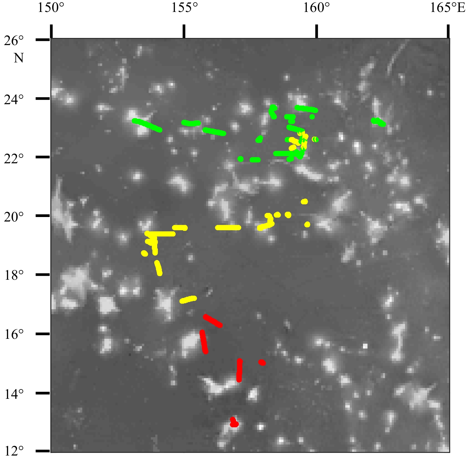
Figure 1. Map of the study area (red box in the insert) and the navigation and acoustic recording route (red line). The study area is located in the seamount (brighter colored areas) region of the northwestern Pacific Ocean.
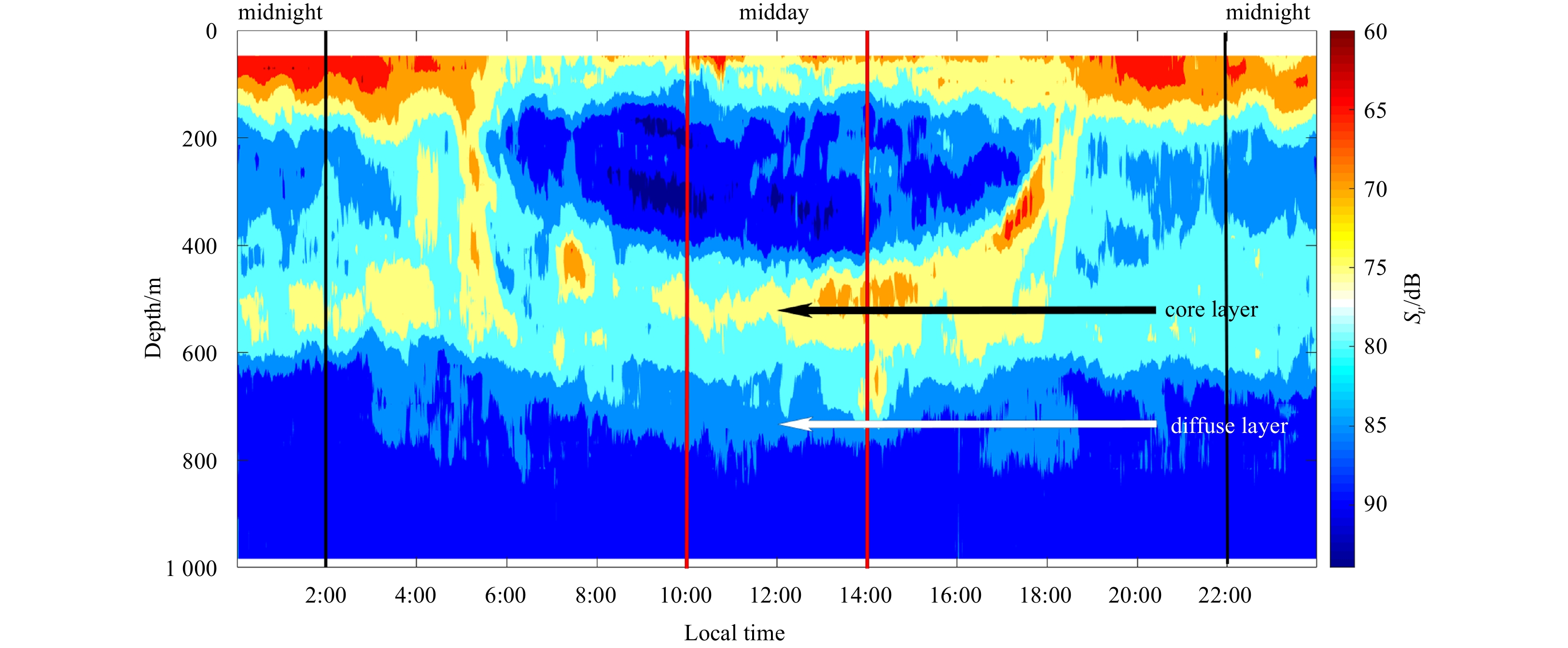
Figure 2. Echogram (38 kHz) after noise-removal showing the diel vertical migration of mesopelagic organisms (at local time 0:00–24:00, September 10, 2018). The red lines indicated the period of midday (at local time 10:00–14:00), when the dwelling depth of mesopelagic organisms was relative stable and it was easy to eliminate the disturbance of diel vertical migration. And the black lines indicated the period of midnight (at local time 22:00–next day 2:00). The black arrow indicated the core part of deep scattering layers (DSLs), and the white arrow indicated the diffuse part of DSLs.
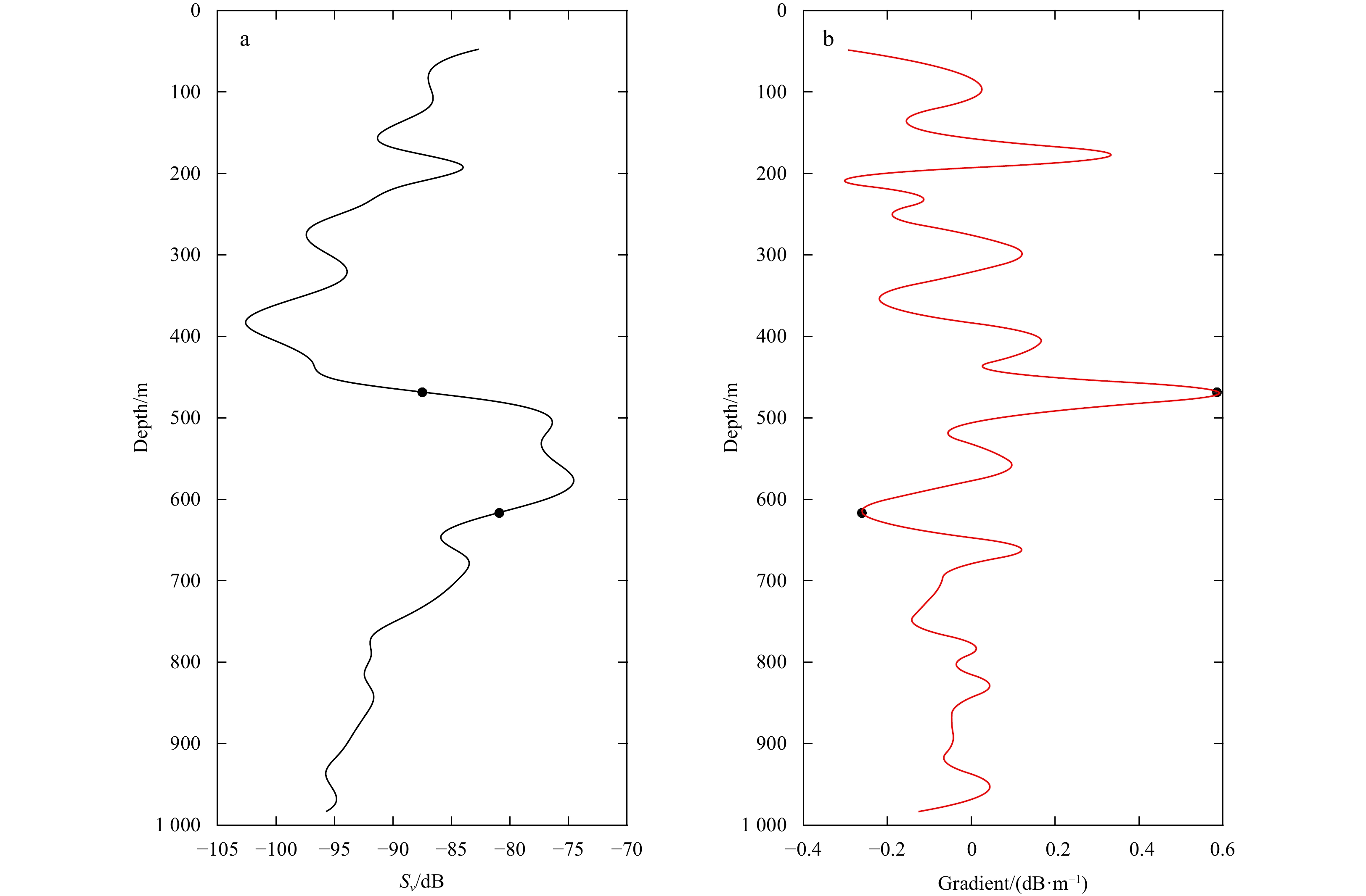
Figure 3. An example about identifying the boundaries of core deep scattering layers (DSLs) according to gradient method. a. Vertical distribution of mean volume backscattering strength (MVBS); b. vertical distribution of changes in gradient of MVBS. The dots are identified boundaries of core DSLs.
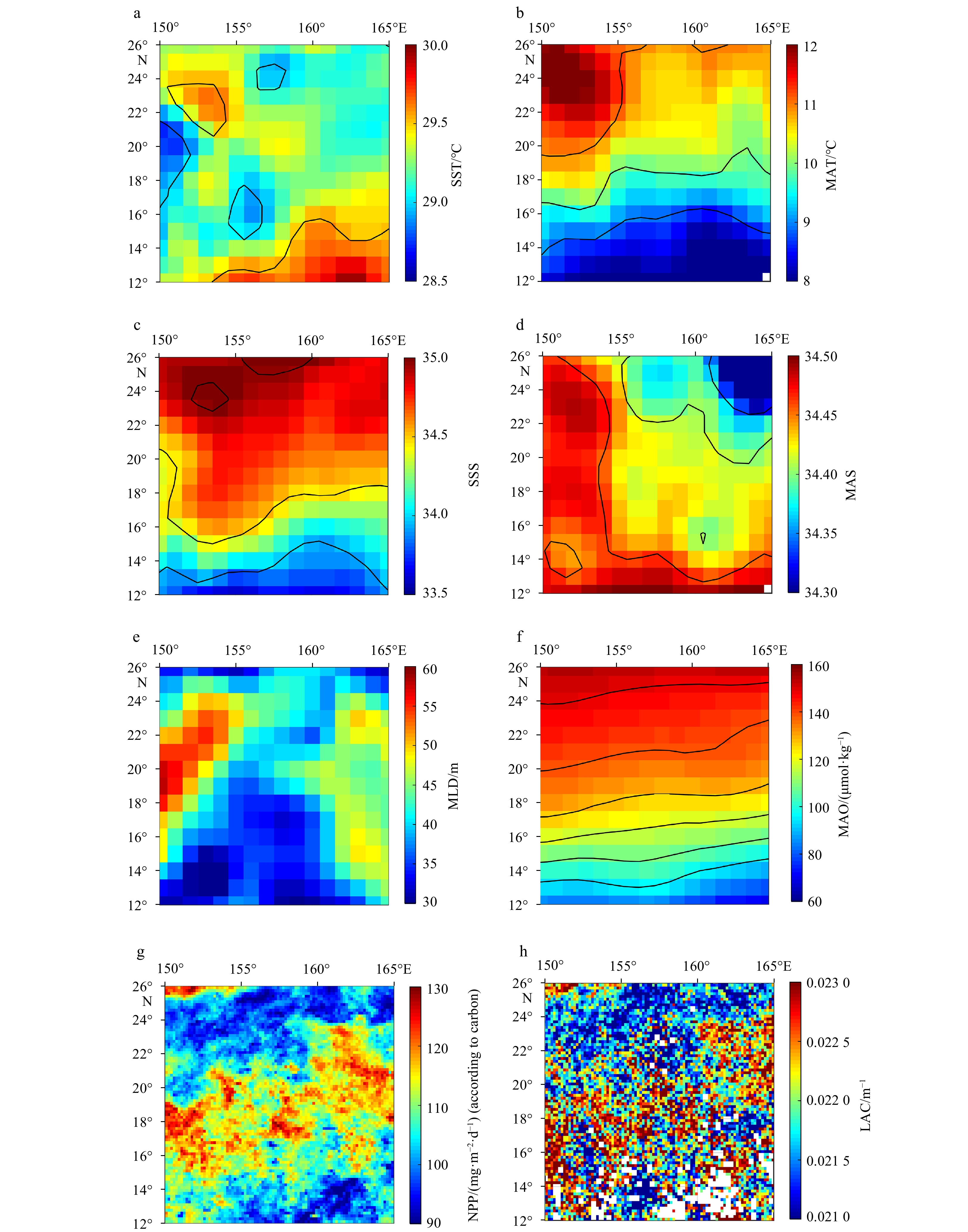
Figure 4. Maps of environmental conditions in the study area (the average data during September was used for mapping). a, b. Sea surface temperature (SST) and mesopelagic average temperature (MAT); c, d. sea surface salinity (SSS) and mesopelagic average salinity (MAS); e. mixing layer depth (MLD); f. mesopelagic average dissolved oxygen concentration (MAO); g. net primary productivity (NPP); h. 490 nm light attenuation coefficient (LAC). The black curves in some images are isolines.
Figure 5. The distribution of environmental variables according to k-means clustering methods in study area. Green group is the northern part, yellow group is the central part, and red group is the southern part.
Figure 6. Box plots about the features of environment in three parts (NP, northern part; CP, central part; SP, southern part). a. Mesopelagic average temperature (MAT); b. mesopelagic average salinity (MAS); c. mesopelagic average dissolved oxygen concentration (MAO); d. 490 nm light attenuation coefficient (LAC); e. primary productivity (PP).
Figure 7. Box plots about the features of deep scattering layers (DSLs), showing the differences among three parts (NP, northern part; CP, central part; SP, southern part). a. Mesopelagic nautical area scattering coefficient (MNASC); b. center mass (CM); and c. mesopelagic gathering level (MGL) of mesopelagic zone. d and e showed the upper (UBD) and lower boundary depth (LBD) of DSLs, respectively.
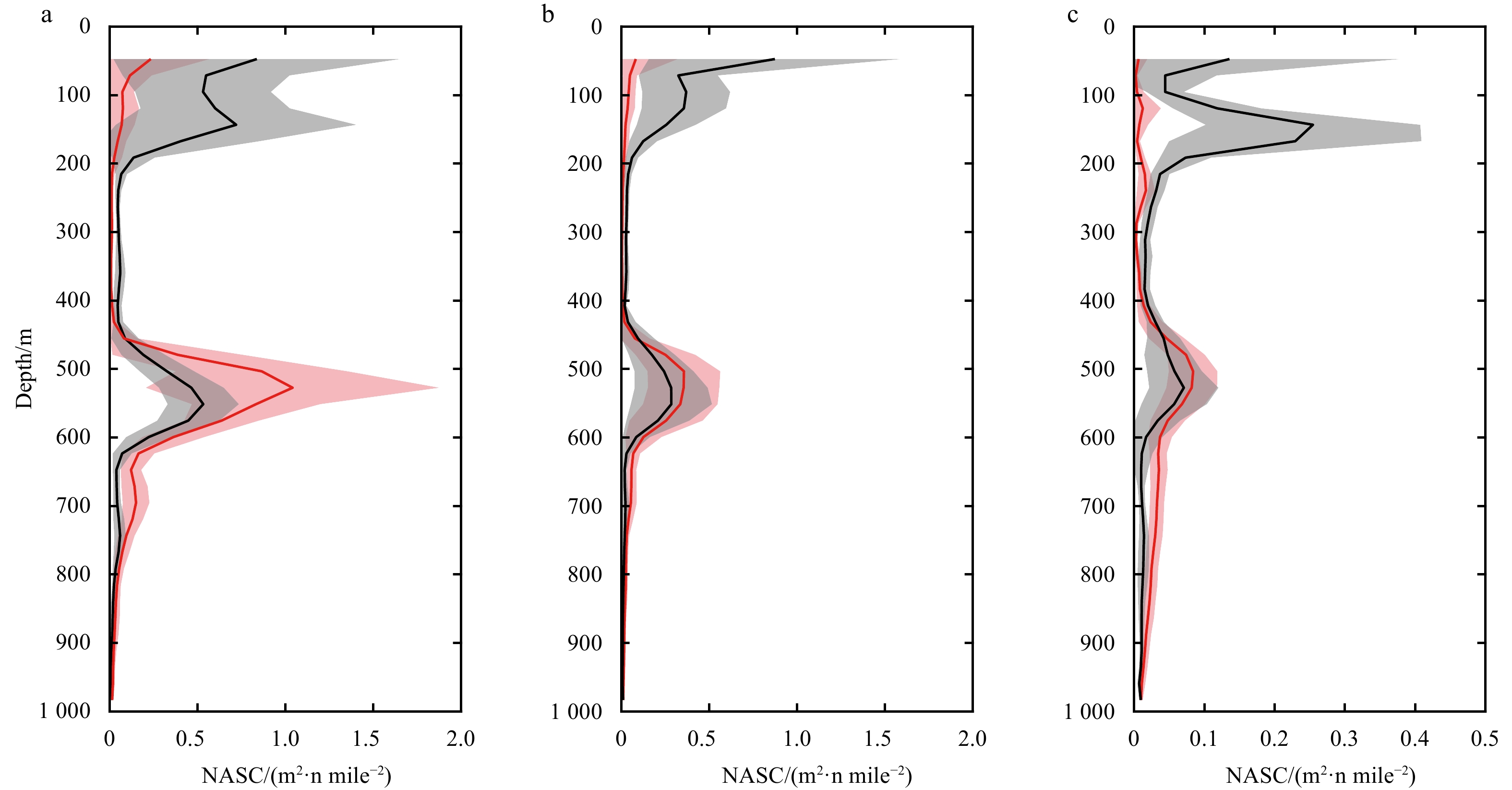
Figure 8. Vertical distribution of acoustic backscatter grouped into three parts, according to the result of k-means cluster analysis. a, northern part; b, central part; c, southern part. Red lines show average midday-time profiles (10:00–14:00), and light red shadows are range of standard deviations. Black lines show average midnight-time profiles (22:00–next day 2:00), and gray shadows are range of standard deviations. x-axis is acoustic backscatter measured as nautical area scattering coefficient (NASC) at the corresponding depth.
Figure 9. The echogram at midday along latitudinal gradient. The yellow curve is 160 μmol/kg dissolved oxygen isoline and the red curve is the depth of 0.01% surface light intensity isoline.
Figure A1. Midday vertical distributions of backscattering strength and its changing gradient in the whole study area. a, b. The vertical distributions of increasing gradient and decreasing gradient, respectively; c. the vertical distribution of mean volume backscattering strength (MVBS). Black curves are identified upper and lower boundaries of DSLs (UBD and LBD). x-axis is the column data number.
Figure A2. The linear correlations between the mesopelagic nautical area scattering coefficient (NASC) during cruise and net primary productivity (NPP) in the past twelve months. The blue lines were fitting curves with R2(p<0.05).
Figure A3. Maps of remote-sensing-based net primary productivity (NPP) in study area during a year (from November 2017 to October 2018).


 DownLoad:


 DownLoad: