
Figure
1.
The Persian Gulf and the computational grid, as well as in situ stations used in this study. WL1−WL10 are tide gauges and V1 and V2 are current velocity stations.
| Citation: | Davood Shariatmadari, Seyed Mostafa Siadatmousavi, Cyrus Ershadi. Numerical study of power production from tidal energy in the Khuran Channel and its feedback on background hydrodynamics[J]. Acta Oceanologica Sinica, 2022, 41(5): 173-182. doi: 10.1007/s13131-021-1968-y

|
Increasing use of fossil fuels has irreversible consequences, such as global warming, ozone depletion, changes in rainfall patterns, rising sea levels, and also detrimental effects on plant, animal, and humans҆ life. Therefore, new and renewable energies are needed to mitigate its harmful effects on the environment. Renewable energies include wind, biomass, ocean, and geothermal energy (Mungar, 2014). With more than 1 500 km of coastline on its southern boundaries, Iran may have a large amount of tidal energy available. Tidal energy is derived from two ways: the potential energy generated by elevations in the sea level and the kinetic energy generated by the current speed. Tidal lagoons built based on the difference between water elevation inside and outside of the lagoon have been used way more than tidal turbines operating based on the current speed. For example, extraction of tidal energy through water level difference was employed in the French La Rance Tidal Power Plant (240 MW, built in 1960). Tidal turbines or tidal energy converters (TECs) consist of several turbines operating independently by the current passing through blades of each turbine. The blades of horizontal-axis tidal turbine convert kinetic energy of the tidal current into mechanical energy by the rods. Power output of tidal turbines depends on intensity of the tidal current. As a result, these turbines are applicable in the areas where tidal speed is high. The minimum peak speed is estimated by ~1 m/s for economically viable running of tidal turbines (Hardisty, 2009).
Several studies have evaluated the potential of extracting energy from tidal current in various parts of the world (Blunden et al., 2013; Blunden and Bahaj, 2007; Chen et al., 2013). The values for turbine thrust coefficients and effects of the turbine farms҆ energy extraction on hydrodynamics in the vicinity of the farm have been studied in detail in some studies (Baston et al., 2015; Ramos and Iglesias, 2013; Waldman et al., 2017) . Also, studying the wake effect generated by the turbines is necessary for characterization of the hydrodynamic effects. Wake analysis shows changes in the mean flow and mixing around the turbine, in addition to its effects farther downstream. The wake extent and its features would influence distribution and efficiency of additional turbines (Mungar, 2014; Neary et al., 2013) and the combined wake of turbine arrays can even influence large-scale hydrodynamics of the environment (Batten et al., 2013; Brown et al., 2017; De Dominicis et al., 2017). There are also several studies on the extraction of energy from the seas around Iran. Ashtari Larki studied the tidal energy inside the Persian Gulf and its availability for extraction along the coasts. In this study, coasts were investigated in terms of tidal currents and tidal amplitude using a numerical model with the finite difference scheme called Coherence (Ashtari, 2012). Khosravi studied the tidal cycle in the Khuran Channel. The across-channel distribution of the mean and tidal flows was obtained over a semidiurnal tidal cycle in the Khuran Channel, where the highest tidal velocity in the third day of the secondary spring tide exceeded 140 cm/s. This study, which was carried out through vessel-mounted ADCP surveys, gives the first detailed description of the mean and tidal current on the high spatial and temporal resolution in this channel (Khosravi et al., 2018).
Accordingly, the present research is carried out to investigate volume of tidal current energy resources that can be exploited and the potential influence of any action taken to extract energy in the area. For this purpose, numerical simulations were done on an assumed tidal farm, in which a 3D hydrodynamic model of the marine area was used based on the measured data. Results of this research can serve as a reference for evaluating extractable reserves and potential effect of this energy in adjacent water bodies.
The Persian Gulf (Fig. 1) located in southwest of Asia is a shallow, semi-confined water body in a semi-arid region. This region with an area of about 230 000 km2 is located in south of Iran. Its width varies between 56 km and 338 km. This area is situated in 24°−30°N and 48°−56°E. The Persian Gulf is connected to the Gulf of Oman and high seas from east by the Strait of Hormuz. The Persian Gulf is one of the most important regions in the world due to economic, political, and military reasons.
Delft3D is a 3D/2D hydrodynamic model consisting of several modules for simulating different processes. The Delft3D-flow module is a part of Delft3D, which deals with large-scale flow simulations. It numerically solves shallow water equations including Navier-Stokes equations. It is applicable for modeling unsteady flow and the results of transition phenomena caused by tidal or meteorological forces including the effects of density changes due to non-uniform temperature and salinity distribution. This model can also be applied to predict flow in shallow water bodies, coastal areas, estuaries, rivers, and lakes (Deltares, 2014).
The governing equations of flow in the sigma coordinates with the hydrostatic pressure condition in shallow water, which include the equations of momentum and continuity, are as follows:
| $$ \begin{split} \frac{{\partial U}}{{\partial t}} + & U\frac{{\partial U}}{{\partial x}} + V\frac{{\partial U}}{{\partial y}} + \frac{w}{h}\frac{{\partial U}}{{\partial \sigma }} - fV = \\ - & \frac{1}{{{\rho _0}}}{P_x} + {F_{x,{\rm{R}}}} + \frac{1}{{{h^2}}}\frac{\partial }{{\partial \sigma }}\left( {{\nu _{\rm{v}} }\frac{{\partial U}}{{\partial \sigma }}} \right), \end{split}$$ | (1) |
| $$\begin{split} \frac{{\partial V}}{{\partial t}} + & U\frac{{\partial V}}{{\partial x}} + V\frac{{\partial V}}{{\partial y}} + \frac{w}{h}\frac{{\partial U}}{{\partial \sigma }} - fU = \\ - & \frac{1}{{{\rho _0}}}{P_y} + {F_{y,{\rm{R}}}} + \frac{1}{{{h^2}}}\frac{\partial }{{\partial \sigma }}\left( {{\nu _{\rm{v}} }\frac{{\partial V}}{{\partial \sigma }}} \right), \end{split}$$ | (2) |
| $$ \frac{\partial \zeta }{\partial t}+ \frac{\partial \left[\left(d+\zeta \right)U\right]}{\partial x} + \frac{\partial \left[\left(d+\zeta \right)V\right]}{\partial x} ={{S_{\rm{D}}}}, $$ | (3) |
where U and V are the horizontal velocity components and w is the vertical velocity component for sigma coordinate, f is the Coriolis parameter,
A large-mesh model with 4 km of spatial resolution on boundaries covering parts of the Gulf of Oman and the entire Persian Gulf was used. This model is referred to as the PG model hereafter. The bathymetry data from the general bathymetric chart of the oceans (GEBCO)-04 database with the resolution of 0.025° were interpolated on a rectangular grid in the PG model. The sigma coordinates with five layers were used in the vertical direction. Along the open boundary, water level was reconstructed using eight tidal components as follows:
| $$ H\left(t\right)={H}_{0}+\sum\limits_{k=1}^{K}{H}_{k}{F}_{k}\mathit{{\rm{cos}}}[{\omega }_{k}t+{\left({V}_{0}+U\right)}_{k}-{G}_{k}], $$ | (4) |
where H(t) is the tidal water elevation at time,
Water level information has been measured at 7 stations in the Persian Gulf area by the Iran National Cartographic Center. Also, the current velocity information was available at two stations from the Port and Maritime Organization. Figure 1 shows the position of the in situ stations. Table 1 provides the details of these stations.
| Observation stations | North latitude/(°) | East longitude/(°) | Measurement period | Depth/m | |
| ID | Name | ||||
| WL1 | Qeshm | 26.937 464 62 | 56.279 568 69 | 1/05/2011−1/06/2011 | |
| WL2 | Rajaie | 27.100 000 00 | 56.066 667 00 | 1/05/2011−1/06/2011 | |
| WL3 | Keshtisazi | 27.033 333 00 | 55.950 000 00 | 1/05/2011−1/06/2011 | |
| WL4 | Bushehr | 28.983 333 00 | 50.833 333 00 | 1/05/2011−1/06/2011 | |
| WL5 | Kangan | 27.833 333 00 | 52.050 000 00 | 1/05/2011−1/06/2011 | |
| WL6 | Dayer | 27.833 333 00 | 51.933 333 00 | 1/05/2011−1/06/2011 | |
| WL7 | Deylam | 30.075 319 86 | 50.093 057 59 | 1/05/2011−1/06/2011 | |
| WL8 | Ganave | 30.419 221 54 | 49.115 414 15 | 1/05/2011−1/06/2011 | |
| WL9 | Lavr | 29.542 620 09 | 50.480 848 23 | 1/05/2011−1/06/2011 | |
| WL10 | Jask | 25.654 908 65 | 57.745 214 20 | 1/05/2011−1/06/2011 | |
| V1 | Bushehr | 28.975 604 70 | 50.859 170 60 | 1/07/2011−1/08/2011 | 10 |
| V2 | Deylam | 29.869 674 00 | 50.120 510 88 | 1/07/2011−1/08/2011 | 25 |
 DownLoad:
CSV
DownLoad:
CSV
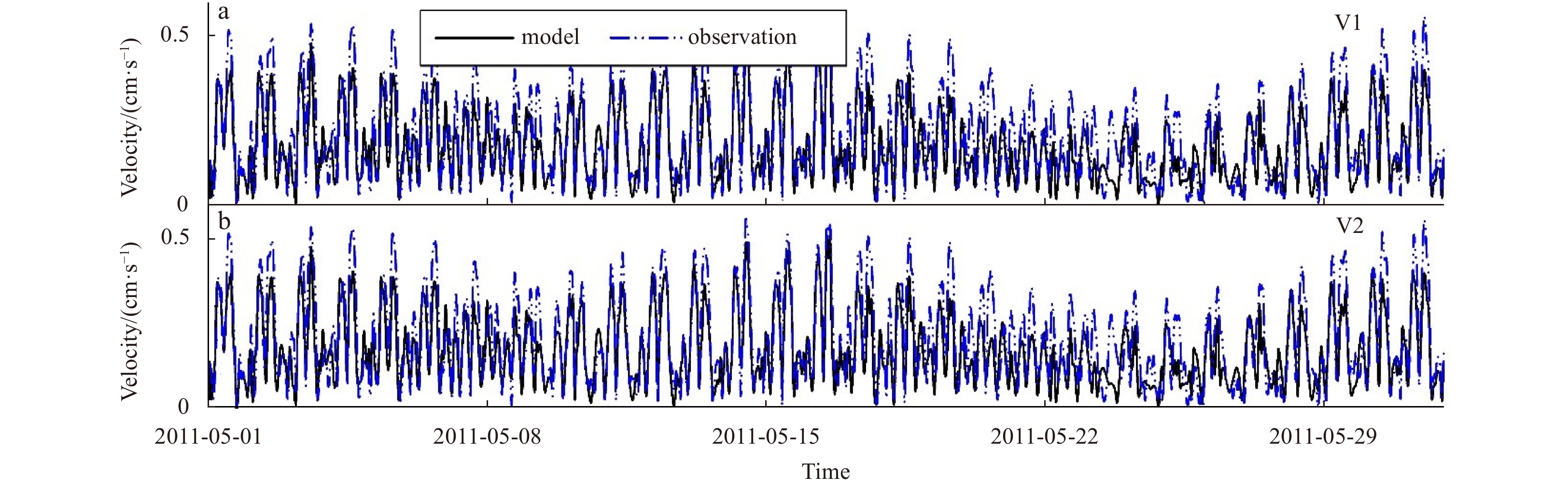
Regarding the period in which the in-situ observations were available (May 2011 for water level and July 2011 for current velocity), the PG model was implemented from May 1 to August 1 2011. The model results for water level and current velocity are shown in Figs 2 and 3. Tables 2 and 3 also show statistics for model assessment. It should be noted that the fact that the current and water level are considered in this study. Therefore, 24 hours were considered to warm up the model. Statistical parameters used for model assessment were the root mean square error (RMSE) and correlation coefficient:


| Observation station | Error analysis | |
| RMSE/m | R | |
| WL1 | 0.235 | 0.948 |
| WL2 | 0.363 | 0.924 |
| WL3 | 0.374 | 0.954 |
| WL4 | 0.184 | 0.924 |
| WL5 | 0.187 | 0.956 |
| WL6 | 0.194 | 0.958 |
| WL7 | 0.307 | 0.91 |
| WL8 | 0.19 | 0.941 |
| WL9 | 0.21 | 0.91 |
| WL10 | 0.06 | 0.995 |
DownLoad:
CSV
| Observation station | Error analysis | |
| RMSE/(m·s-1) | R | |
| V1 | 0.08 | 0.931 |
| V2 | 0.05 | 0.910 |
DownLoad:
CSV
| $$ \mathrm{R}\mathrm{M}\mathrm{S}\mathrm{E}=\sqrt{\frac{1}{{N}}\sum _{{n}=1}^{{N}}{({{O}}_{{n}}-{{M}}_{{n}})}^{2}}, $$ | (5) |
| $${R} = \frac{{\displaystyle\frac{1}{{{N}}}\displaystyle\sum _{{{n}} = 1}^{{N}}({{{O}}_{{{n}} }}- {{{\bar{O}}_{{n}}})} ({{{M}}_{{{n}} - }} {{{\bar{M}}_{{n}}})} }}{{{\sigma _{\rm{O}}}\cdot{\sigma _{\rm{M}}}}}, $$ | (6) |
where N is the number of measurements, n is the data counter,
Figure 2 shows the results obtained from comparison of water level from the model with observations at the measurement stations in the PG model. These comparisons are also summarized in Table 2 using the statistical indices. According to the results, the correlation coefficient between the results is right and there is a good agreement between time series of water level from the station and outputs of the numerical model at all stations. Figure 3 shows times series of the current speed at Bushehr station (with 10 m of depth) and at Deylam station (with 25 m of depth) using the results of the numerical model. The statistics are also presented in Table 3. Results obtained from Bushehr station were found to be better than those of Deylam station, but the overall performance of the model for estimating the current velocity was slightly lower for estimating the water level. It might be due to some factors, such as tidal flux errors, floor friction coefficient, depth resolution or ignoring factors, such as wave and sediment transport. In general, despite these deviations, the model is considered suitable for predicting effective distribution of tidal currents and water level within the Persian Gulf.
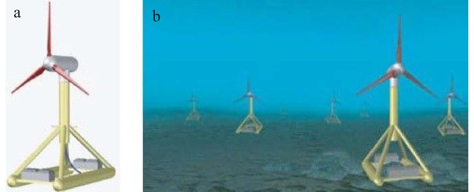
There are several designs of TECs, and an overview of these systems can be found on the European marine energy center (EMEC) website (Tidal clients, 2013). A list of tidal turbine developers can also be found in the literature (Hardisty, 2009). However, to date, the horizontal-axis tidal turbine is the most standard design of such a converter as shown in Fig. 4, which converts current energy into rotating motion to generate electricity (Bir et al., 2011).

The present version of Delft3D does not include any specific concepts for defining tidal turbines. One method to include the turbine feedback on the hydrodynamic in this software is to add momentum loss expression to the governing equations to simulate the energy extraction from the current field (Batten et al., 2013). In this method, Eqs (1) and (2) are rewritten as follows:
| $$ \begin{split} \frac{{\partial {{U}}}}{{\partial {{t}}}} + & U\frac{{\partial {{U}}}}{{\partial {{x}}}} + v\frac{{\partial {{U}}}}{{\partial {{y}}}} + \frac{w}{h}\frac{{\partial U}}{{\partial \sigma }} - fV = \\ - & \frac{1}{{{\rho _0}}}{P_x} + {F_{x.R}} + \frac{1}{{{h^2}}}\frac{\partial }{{\partial \sigma }}\left( {{\nu _{\rm{v}} }\frac{{\partial U}}{{\partial \sigma }}} \right) + {M_x,} \end{split} $$ | (7) |
| $$\begin{split} \frac{{\partial {{V}}}}{{\partial {{t}}}} + & U\frac{{\partial {{V}}}}{{\partial {{x}}}} + v\frac{{\partial {{V}}}}{{\partial {{y}}}} + \frac{w}{h}\frac{{\partial U}}{{\partial \sigma }} - fU = \\ - & \frac{1}{{{\rho _0}}}{P_y} + {F_{{{y}},{\rm{R}}}} + \frac{1}{{{h^2}}}\frac{\partial }{{\partial \sigma }}\left( {{\nu _{\rm{v}} }\frac{{\partial V}}{{\partial \sigma }}} \right) + {M_y,} \end{split} $$ | (8) |
where
| $$ {M}_{x} = {C}_{{\rm{loss}}-U} \frac{{U}^{2}}{{\mathrm{\Delta }}_{x}}, $$ | (9) |
| $$ {M}_{y} = {C}_{{\rm{loss}}-V} \frac{{V}^{2}}{{\mathrm{\Delta }}_{y}}. $$ | (10) |
For this research, the turbines were simulated by introducing a series of porous plates into the following model (Baston et al., 2015; Mungar, 2014). These plates are applied to the layers containing porous PGs based on the
| $$ {C}_{{\rm{loss}}-U} = \frac{{C}_{{\rm{T}}}{A}_{U}}{2{\mathrm{\Delta }}_{y}{\mathrm{\Delta }}_{Zn}}, $$ | (11) |
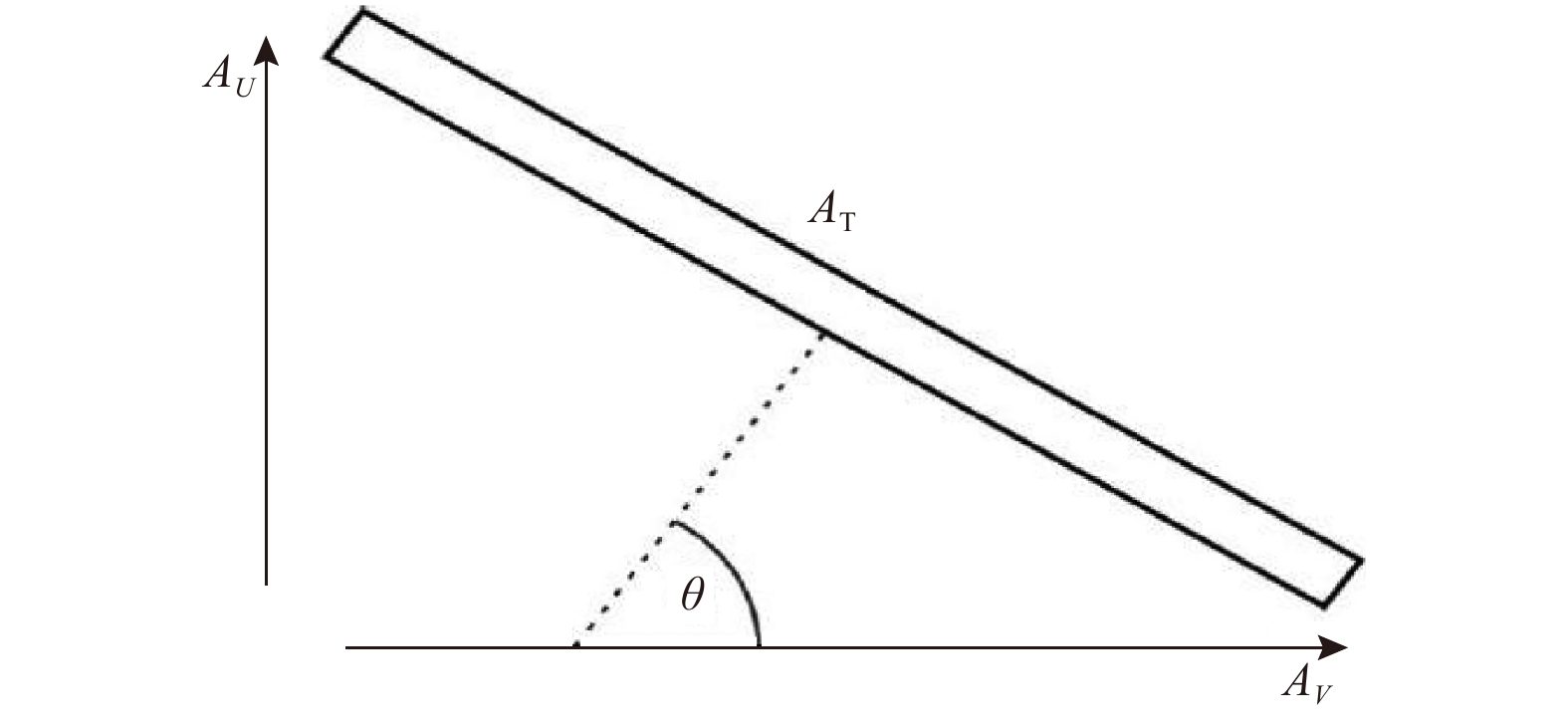
| $$ {A}_{U} = \sum {A}_{{\rm{T}}}\left|\mathrm{sin}\theta \right|, $$ | (12) |
where

The following method can be used to calculate the output power of each turbine in the tidal farm.
| $$ {P}_{{\rm{device}}}={P}_{{\rm{m}}} A \eta, $$ | (13) |
where A is the area swept by the rotation of the blades of each turbine, η is the turbine efficiency coefficient (0.3 is considered), and Pm is the average tidal density of energy available to each turbine determined by the following equation:
| $$ {P}_{{\rm{m}}}= \frac{1}{2T} \rho {\int }_{0}^{T}{\left|{U}_{{\rm{T}}}\right|}^{3}{{\rm{d}}}{t} \quad {\rm{when}}\;{U}_{{\rm{T}}} > 1 ,$$ | (14) |
where T is the main tidal period in the region, ρ is the sea surface density, and UT denotes the velocity vector along the turbine axis. The calculations were performed assuming the velocity required to start the turbine is 1 m/s. It should be noted that the tidal velocity varies with time, and its average velocity over a period is determined as follows:
| $$ {U}_{{\rm{T}}} = \frac{{\sum\limits_{\sigma =a}^{\sigma =b}}{U}_{\sigma }}{\left|b-a\right|} ,$$ | (15) |
where
Model results presented here include co-tidal charts and tidal ellipses for main tidal constituents. The main tidal components considered here are M2, S2, K1 and O1 as presented in Fig. 6.

The co-tidal charts show two amphidromic points observed for each semidiurnal component and one amphidromic point for each diurnal components in the Persian Gulf. An amphidromic point is a point where the tidal fluctuation is almost zero for considered constituent. Its location depends on the Coriolis and bathymetry effects. The semidiurnal co-amplitudes of M2 and S2 have similar paterns but they are not of the same range. The amplitude of M2 is almost twice as large as the amplitude of S2 (Figs 6 a and b). The co-amplitudes of diurnal components K1 and O1 are similar in range and also in pattern, except close to the Strait of Hormuz (Figs 6c and d).
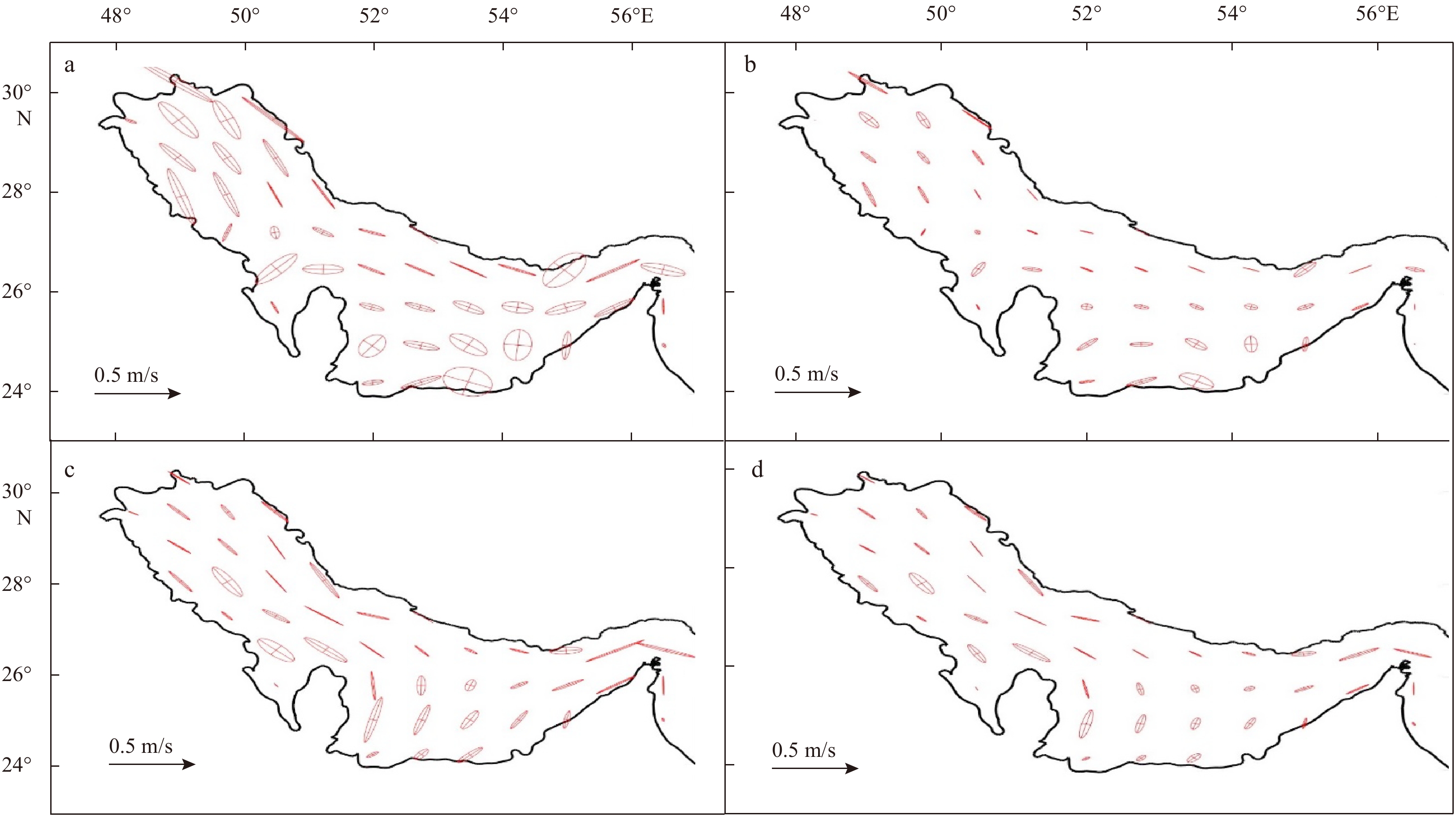
One of the most important tools for studying tidal currents is presenting tidal ellipses over the study area. These ellipses are drawn in proportion to the changes in speed and direction of tidal flow at each location. The major axis of the tidal ellipse shows the maximum tidal velocity in the tidal cycle. In contrast, its small axis shows the minimum tidal vector in the same cycle.
Figure 7 show tidal ellipses for different regions of the Persian Gulf for main tidal components. They are almost bidirectional linear pattern at northern part of the Persian Gulf. As shown in Fig 7a, the maximum velocity of M2 varies at different points. The currents are stronger in the north-west part of the Perian Gulf while they are weak near the amphiphromic points. As designated in Fig 7b, the tidal ellipse of S2 are similar in pattern but weaker in speed than that of M2. In the case of the maximum tidal velocity for the K1 and O1 components, the situation is quite different as shown in Fig 7d. Relatively high velocities are clearly visible in the western part of the Strait of Hormuz for these diurnal components.

In fact, the orientation of diurnal and semi-dirunal compents are different in the southern part of the Persian Gulf while they are similar to each other for the northern parts.
A well-calibrated model can be used to determine the locations with the highest current velocity along the Persian Gulf coast. The four regions with the highest current energy were identified, which are illustrated in Fig. 8. Zone 1 is not desirable in terms of large current and the expected energy, which can be extracted. The maximum current velocity is about 0.8 m/s. Zone 2 has a maximum current velocity of more than 1 m/s. It is favorable in terms of size and current durability. It can be used as one of the sources of energy production. However, there is a possibility of interference with transportation. As mentioned in Introduction Section, significant traffic of oil tankers exists in this zone. There is not very high current velocity at Zone 3. The maximum tidal current velocity in this zone is approximately 1 m/s. Based on the previous studies (Ashtari, 2012), the tidal range in this zone is more than 4 m. It has numerous waterways, some of which are used for shipping, and there is a high possibility of interference between shipping and turbine performance. Also, it is possible to construct the lagoon in this zone. Zone 4 is favorable in terms of durability and large current velocity, and it can be used as a suitable location for generating energy by tidal turbines, depending on topography of the area.

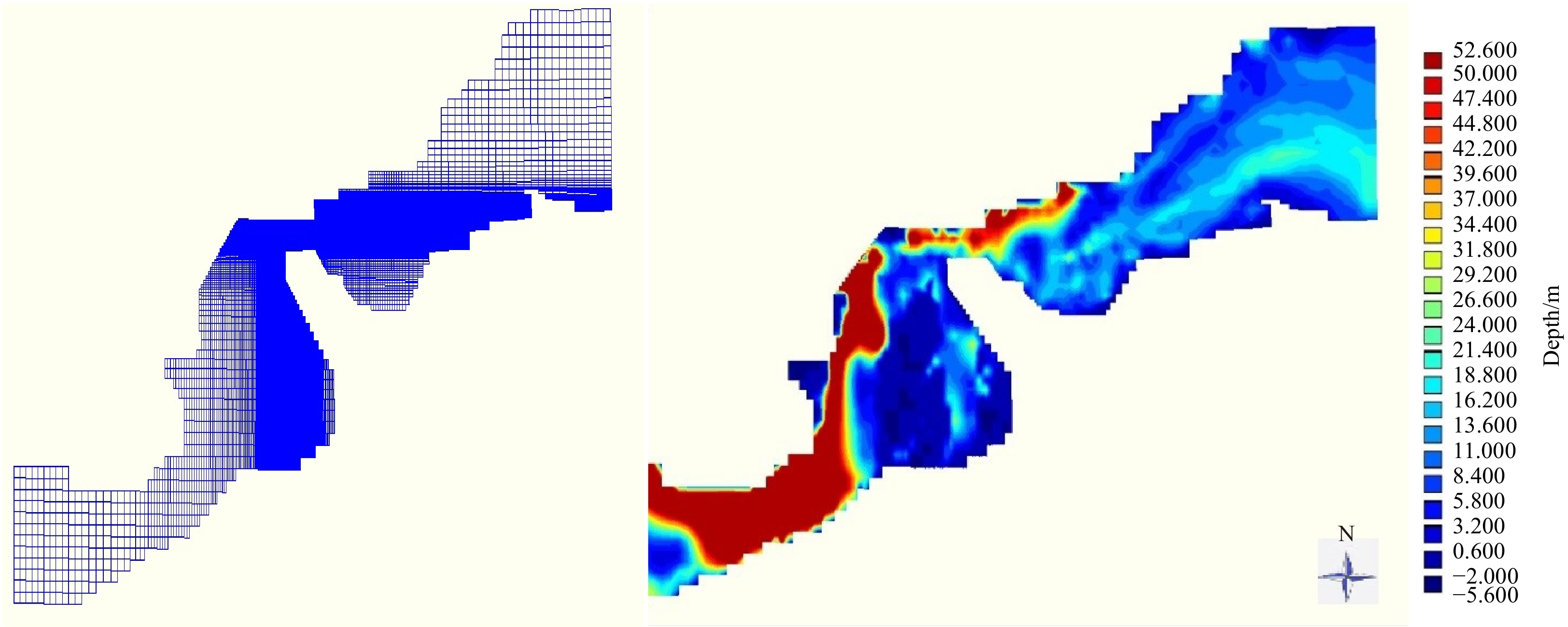
The Khuran Channel, located in Zone 4, is a 115 km long waterway between Qeshm Island and Iranian Plateau as shown in Fig. 9. Its width is equal to 22 km in the eastern entrance, which is decreased to 2.5 km in the middle of the channel. Then, it reaches to 10 km at the western part, where it joins the Persian Gulf (Ashtari, 2012). The local model for this channel is called as the QC model hereafter. It is a rectangular fine grid model that covers the space between Qeshm Island and the Iranian Coast. The grid has a spatial resolution of ~200 m around the boundaries, and this distance reaches to 20 m near high tide-prone locations as shown in Fig. 9. Two independent models of PG and QC were used in order to optimize simulation run time. At open boundaries of QC model, the time series of water level were extracted from the PG model. Time step of the QC model was set as 6 s. Also, the QC modeling details are similar to the PG model.

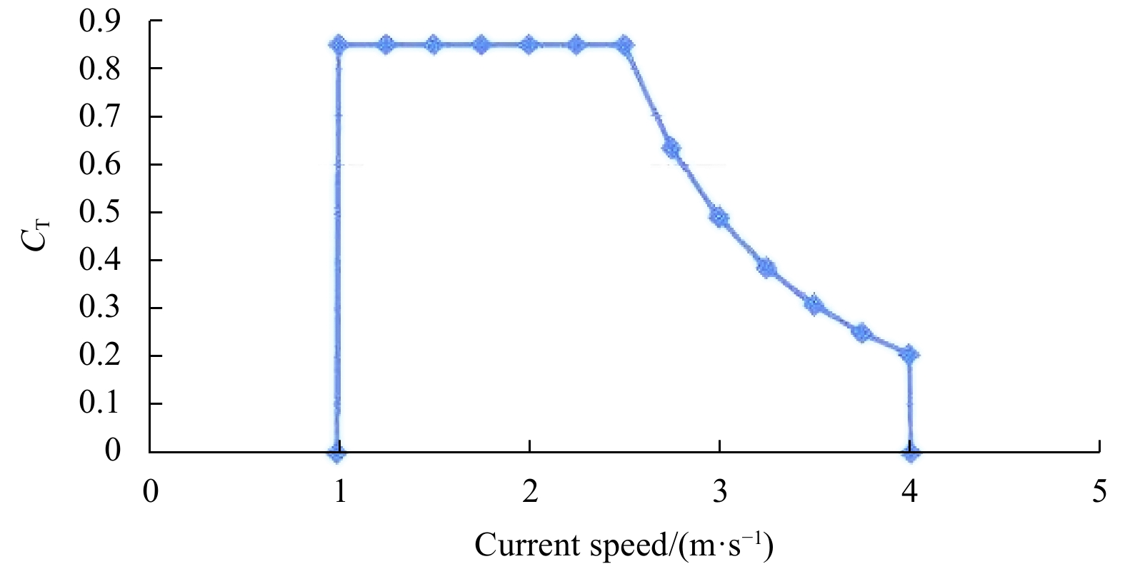
According to the TEC developers, the thrust coefficient parameter is demonstrated in Fig. 10 for a tidal turbine with the following specifications: rotator diameter of 20 m, initial starting velocity of 1 m/s, nominal velocity of 2.5 m/s, and final velocity of 4 m/s (Bahaj et al., 2007).

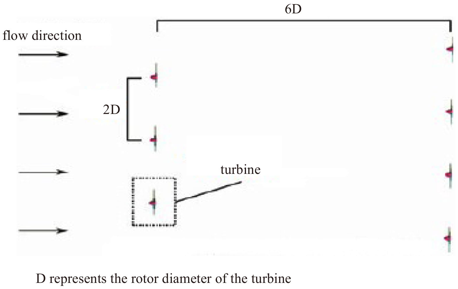
According to Figs 11a and b , the simulated velocity shows considerable asymmetry during spring ebb and spring flood tides, with the maximum velocities about 2.1 m/s and 1.6 m/s, respectively. The thickness of sigma layers in the 3D model varies with time, so deployment of the turbine in the specified layers is not reasonable. According to the lowest water level, the horizontal-axis tidal turbine is fixed at 3 m below the average water surface. Therefore, an area of 980 m × 420 m was selected with a depth ranging from 27 m to 40 m. According to the EMEC standard, the horizontal-axis tidal turbines with a diameter of 20 m were selected (Black & Veatch Consulting, Ltd., 2009). The Staggered Arrangement was used to realize a multiple-row array, as shown in Fig. 12. Lateral spacing of the turbines was twice the diameter of the turbine in the horizontal-axis tidal farm, and longitudinal distance of the turbines was six times the diameter of the turbine. Considering the highest tidal velocity in the study area, which is equal to 2.1 m/s, the turbines were set up as 9 turbines per row with 11 columns; therefore, a total of 99 turbines were placed in the area of 411 600 m2. Figure 13 demonstrates the average daily power production of the tidal farm over one month. Monthly average power production was approximately 1.3 MW.


After the tidal farm was established, and energy of the tidal farm was extracted at this stage, the effects of this farm on hydrodynamics of the surrounding environment were also investigated. For assessing these effects, the QC model was set up with and without turbines. This model was run for 30 days including two spring-neap tidal cycles.
According to Fig. 14, the difference in water level shows that a hypothetical tidal farm would influence the sea level over a large area. The water level fluctuations around the tidal farm are 4 cm, which reaches a maximum of 8 cm near the shores.

In addition to the difference in current velocity, Fig. 15 illustrates that tidal speed would drop significantly close to tidal farm. The maximum drop occurs on the side near the coast and it is more than 0.8 m/s. The effects of these velocity changes also convey up to ~7 km downstream. However, on both sides of the tidal farm, there is a noticeable increase in the current velocity due to the blockage effects, which is much more evident on the shore side and this may increase the coastal erosion in the area.

Based on the results of our analysis, the assumed tidal farm and its corresponding current intensity might dramatically change tidal characteristics inside the Khuran Channel. As a beautiful natural place, this island is the home for a large number of water birds, so the farm may significantly influence its ecological environment. Therefore, it is of great importance to combine technical feasibility and environmental tolerance in any plan for development of tidal energy.
A 3D hydrodynamic model with the Delft3D-flow module was implemented for the Persian Gulf. This model well illustrates the nature of tides in the Persian Gulf. After validation of the model results, the points with potential for energy extraction in the Persian Gulf were identified. The Khuran Channel was one of the suitable points for extraction of tidal energy, which was studied in more details using a high-resolution local 3D model. A momentum sink term was added to the momentum equations to show the effects of tidal turbines on the local hydrodynamic. Using this method and through creation of a tidal farm with 99 turbines, the potential energy, which can be extracted from the tidal current in the Khuran Channel was estimated as 1.3 MW per day for the area of 411 600 m2.
Then, the effects of this tidal farm on water level and current velocity were evaluated. The water level fluctuations were ~4 cm, but they reached to 8 cm near the coasts. Drop in the current velocity caused by the tidal farms҆ wake was ~0.8 m/s, and range of the effect of this drop could be observed up to ~7 km downstream of the tidal farm.
| [1] |
Ashtari L A. 2012. Study of tidal energy potential in Iranian coasts of the Persian Gulf [dissertation]. Khorramshahr: Khorramshahr University of Marine Science and Technology
|
| [2] |
Bahaj A S, Molland A F, Chaplin J R, et al. 2007. Power and thrust measurements of marine current turbines under various hydrodynamic flow conditions in a cavitation tunnel and a towing tank. Renewable Energy, 32(3): 407–426,doi: 10.1016/j.renene.2006.01.012
|
| [3] |
Baston S, Waldman S M, Side J C. 2015. Modelling energy extraction in tidal flows. In: TeraWatt Position Paper, Revision 3.1. MASTS, 75–107,doi: 10.13140/RG.2.1.4620.2481
|
| [4] |
Batten W M J, Harrison M E, Bahaj A S. 2013. Accuracy of the actuator disc-RANS approach for predicting the performance and wake of tidal turbines. Philosophical Transactions of the Royal Society A: Mathematical, Physical and Engineering Sciences, 371(1985): 20120293,
|
| [5] |
Bir G S, Lawson M J, Li Ye. 2011. Structural design of a horizontal-axis tidal current turbine composite blade. In: ASME 30th International Conference on Ocean, Offshore, and Arctic Engineering. Rotterdam, The Netherlands: NREL
|
| [6] |
|
| [7] |
Blunden L S, Bahaj A S. 2007. Effects of tidal energy extraction at Portland Bill, southern UK predicted from a numerical model. In: Proceedings of the 7th European Wave and Tidal Energy Conference. Porto, Portugal
|
| [8] |
Blunden L S, Bahaj A S, Aziz N S. 2013. Tidal current power for Indonesia? An initial resource estimation for the Alas Strait. Renewable Energy, 49: 137–142,doi: 10.1016/j.renene.2012.01.046
|
| [9] |
Brown A J G, Neill S P, Lewis M J. 2017. Tidal energy extraction in three-dimensional ocean models. Renewable Energy, 114: 244–257,doi: 10.1016/j.renene.2017.04.032
|
| [10] |
Chen Weibo, Liu Wencheng, Hsu M H. 2013. Modeling assessment of tidal current energy at Kinmen Island, Taiwan. Renewable Energy, 50: 1073–1082,doi: 10.1016/j.renene.2012.08.080
|
| [11] |
De Dominicis M, Murray R O, Wolf J. 2017. Multi-scale ocean response to a large tidal stream turbine array. Renewable Energy, 114: 1160–1179,doi: 10.1016/j.renene.2017.07.058
|
| [12] |
Deltares. 2014. Delft3D-FLOW User Manual, Hydro-Morphodynamics, Version 3.15. 34158. Technical Report. http://content.oss.deltares.nl/delft3d/manuals/Delft3D-FLOW_User_Manual.pdf [2014-06-01/2021-01-03]
|
| [13] |
Hardisty J. 2009. Australia and New Zealand. In: The Analysis of Tidal Stream Power. Chichester: John Wiley & Sons Inc, 233−248,
|
| [14] |
Khosravi M, Siadat Mousavi S M, Chegini V, et al. 2018. Across-channel distribution of the mean and tidal flows in the Khuran Channel, Persian Gulf, Iran. International Journal of Maritime Technology, 10: 1-6,doi: 10.29252/ijmt.10.1
|
| [15] |
Mungar S. 2014. Hydrodynamics of horizontal-axis tidal current turbines: A modelling approach based on Delft3D [dissertation]. Delft, Netherlands: Delft University of Technology
|
| [16] |
Neary V S, Gunawan B, Hill C, et al. 2013. Near and far field flow disturbances induced by model hydrokinetic turbine: ADV and ADP comparison. Renewable Energy, 60: 1–6,doi: 10.1016/j.renene.2013.03.030
|
| [17] |
Ramos V, Iglesias G. 2013. Performance assessment of Tidal Stream Turbines: A parametric approach. Energy Conversion and Management, 69: 49–57,doi: 10.1016/j.enconman.2013.01.008
|
| [18] |
Tidal clients. EMEC: European Marine Energy Centre. http://www.emec.org.uk/about-us/our-tidal-clients/ [2013-11-25/2021-03-30]
|
| [19] |
Waldman S, Bastón S, Nemalidinne R, et al. 2017. Implementation of tidal turbines in MIKE 3 and Delft3D models of Pentland Firth & Orkney Waters. Ocean & Coastal Management, 147: 21–36,doi: 10.1016/j.ocecoaman.2017.04.015
|
| 1. | Juan Gabriel Rueda-Bayona, José Luis García Vélez, Daniel Mateo Parrado-Vallejo. Effect of Sea Level Rise and Access Channel Deepening on Future Tidal Power Plants in Buenaventura Colombia. Infrastructures, 2023, 8(3): 51. doi:10.3390/infrastructures8030051 |

Figures(15) / Tables(3)

Supported by:
Beijing Renhe Information Technology Co. Ltd

Davood Shariatmadari, Seyed Mostafa Siadatmousavi, Cyrus Ershadi. Numerical study of power production from tidal energy in the Khuran Channel and its feedback on background hydrodynamics[J]. Acta Oceanologica Sinica, 2022, 41(5): 173-182. doi: 10.1007/s13131-021-1968-y

| Observation stations | North latitude/(°) | East longitude/(°) | Measurement period | Depth/m | |
| ID | Name | ||||
| WL1 | Qeshm | 26.937 464 62 | 56.279 568 69 | 1/05/2011−1/06/2011 | |
| WL2 | Rajaie | 27.100 000 00 | 56.066 667 00 | 1/05/2011−1/06/2011 | |
| WL3 | Keshtisazi | 27.033 333 00 | 55.950 000 00 | 1/05/2011−1/06/2011 | |
| WL4 | Bushehr | 28.983 333 00 | 50.833 333 00 | 1/05/2011−1/06/2011 | |
| WL5 | Kangan | 27.833 333 00 | 52.050 000 00 | 1/05/2011−1/06/2011 | |
| WL6 | Dayer | 27.833 333 00 | 51.933 333 00 | 1/05/2011−1/06/2011 | |
| WL7 | Deylam | 30.075 319 86 | 50.093 057 59 | 1/05/2011−1/06/2011 | |
| WL8 | Ganave | 30.419 221 54 | 49.115 414 15 | 1/05/2011−1/06/2011 | |
| WL9 | Lavr | 29.542 620 09 | 50.480 848 23 | 1/05/2011−1/06/2011 | |
| WL10 | Jask | 25.654 908 65 | 57.745 214 20 | 1/05/2011−1/06/2011 | |
| V1 | Bushehr | 28.975 604 70 | 50.859 170 60 | 1/07/2011−1/08/2011 | 10 |
| V2 | Deylam | 29.869 674 00 | 50.120 510 88 | 1/07/2011−1/08/2011 | 25 |
DownLoad:
CSV
| Observation station | Error analysis | |
| RMSE/m | R | |
| WL1 | 0.235 | 0.948 |
| WL2 | 0.363 | 0.924 |
| WL3 | 0.374 | 0.954 |
| WL4 | 0.184 | 0.924 |
| WL5 | 0.187 | 0.956 |
| WL6 | 0.194 | 0.958 |
| WL7 | 0.307 | 0.91 |
| WL8 | 0.19 | 0.941 |
| WL9 | 0.21 | 0.91 |
| WL10 | 0.06 | 0.995 |
DownLoad:
CSV
| Observation station | Error analysis | |
| RMSE/(m·s-1) | R | |
| V1 | 0.08 | 0.931 |
| V2 | 0.05 | 0.910 |
DownLoad:
CSV
| Observation stations | North latitude/(°) | East longitude/(°) | Measurement period | Depth/m | |
| ID | Name | ||||
| WL1 | Qeshm | 26.937 464 62 | 56.279 568 69 | 1/05/2011−1/06/2011 | |
| WL2 | Rajaie | 27.100 000 00 | 56.066 667 00 | 1/05/2011−1/06/2011 | |
| WL3 | Keshtisazi | 27.033 333 00 | 55.950 000 00 | 1/05/2011−1/06/2011 | |
| WL4 | Bushehr | 28.983 333 00 | 50.833 333 00 | 1/05/2011−1/06/2011 | |
| WL5 | Kangan | 27.833 333 00 | 52.050 000 00 | 1/05/2011−1/06/2011 | |
| WL6 | Dayer | 27.833 333 00 | 51.933 333 00 | 1/05/2011−1/06/2011 | |
| WL7 | Deylam | 30.075 319 86 | 50.093 057 59 | 1/05/2011−1/06/2011 | |
| WL8 | Ganave | 30.419 221 54 | 49.115 414 15 | 1/05/2011−1/06/2011 | |
| WL9 | Lavr | 29.542 620 09 | 50.480 848 23 | 1/05/2011−1/06/2011 | |
| WL10 | Jask | 25.654 908 65 | 57.745 214 20 | 1/05/2011−1/06/2011 | |
| V1 | Bushehr | 28.975 604 70 | 50.859 170 60 | 1/07/2011−1/08/2011 | 10 |
| V2 | Deylam | 29.869 674 00 | 50.120 510 88 | 1/07/2011−1/08/2011 | 25 |
| Observation station | Error analysis | |
| RMSE/m | R | |
| WL1 | 0.235 | 0.948 |
| WL2 | 0.363 | 0.924 |
| WL3 | 0.374 | 0.954 |
| WL4 | 0.184 | 0.924 |
| WL5 | 0.187 | 0.956 |
| WL6 | 0.194 | 0.958 |
| WL7 | 0.307 | 0.91 |
| WL8 | 0.19 | 0.941 |
| WL9 | 0.21 | 0.91 |
| WL10 | 0.06 | 0.995 |
| Observation station | Error analysis | |
| RMSE/(m·s-1) | R | |
| V1 | 0.08 | 0.931 |
| V2 | 0.05 | 0.910 |
 DownLoad:


 DownLoad: