Figure
1.
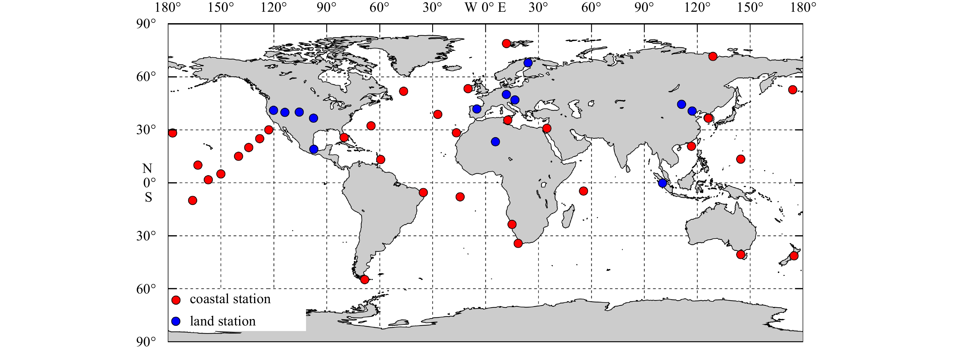
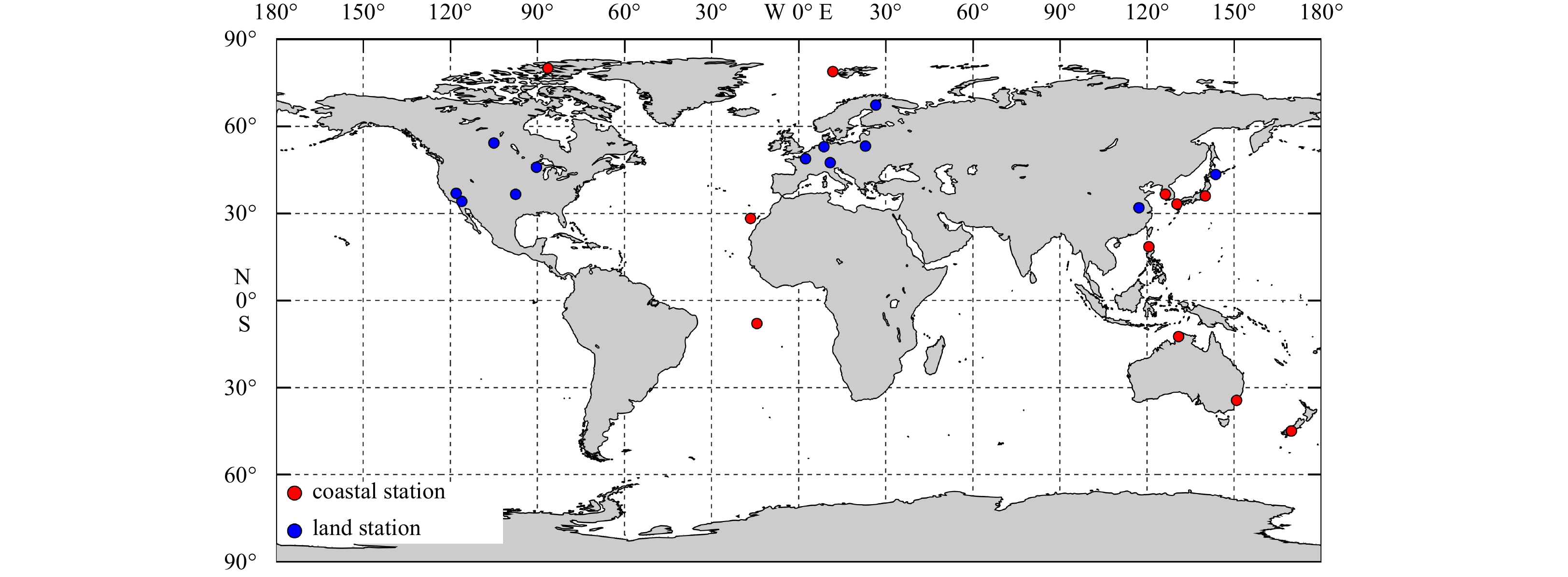
Locations of the Total Carbon Column Observing Network stations with matchups to OCO-2 XCO2 products.
| Citation: | Siqi Zhang, Yan Bai, Xianqiang He, Haiqing Huang, Qiangkun Zhu, Fang Gong. Comparisons of OCO-2 satellite derived XCO2 with in situ and modeled data over global ocean[J]. Acta Oceanologica Sinica, 2021, 40(4): 136-142. doi: 10.1007/s13131-021-1844-9

|
Due to the utilization of fossil fuels and changes in land use, atmospheric CO2 has continued to increase since the industrial revolution, which has profound impact on earth carbon cycle and global warming (IPCC, 2013). Accurate observations of atmospheric CO2 with high spatiotemporal resolution are the basis for estimating air-sea CO2 flux (Bai et al., 2015; Song et al., 2016), understanding long-term changes and improving our ability to predict and mitigate climate change (Intergovernmental Panel on Climate Change, 2007; Jenkinson et al., 1991). Understanding the global atmospheric carbon dioxide concentration, especially the atmospheric carbon dioxide change over the ocean, is an important reference for many global climate changes above. Currently, there are several ways to obtain dry-air mole fractions of atmospheric CO2 (XCO2), including in situ measurements, remote sensing and modeling simulation. In situ measurements generally provide the best quality CO2 concentrations, but the number of ground-based sites is limited, resulting in the absence of data in many global areas, especially in oceanic regions (Bousquet et al., 2006; Eldering et al., 2017). In contrast, space-borne detection is the most effective technical method to observe atmospheric XCO2 with long time series and global coverage. For example, the Scanning Imaging Absorption Spectrometer for Atmospheric Chartography launched in 2002 was the first space-based instrument to retrieve atmospheric XCO2 (Bovensmann et al., 1999; Buchwitz et al., 2007). Launched in April 2009, the Greenhouse Gases Observing Satellite (GOSAT) provides a more accurate atmospheric XCO2 product, at a precision of around 0.6% (Cogan et al., 2012; Joiner et al., 2011; Yokota et al., 2009), as does GOSAT-2, which was launched in October 2018. Especially, NASA launched the Orbiting Carbon Observatory-2 (OCO-2) on 2 July 2014 to provide an atmospheric XCO2 product with higher accuracy (Crisp, 2015). In addition, China launched TANSAT satellite in December 2016 to measure atmospheric XCO2.
Satellite remote sensing of atmospheric XCO2 is still in the developing stage, especially in regard to validation of satellite-derived XCO2 products on a global scale. The principal challenge is the need for unprecedented levels of precision and accuracy to resolve long-term changes and quantify CO2 flux; however, as an indirect observation, the accuracy of satellite detection is limited by inversion algorithms. Moreover, the validation of XCO2 products often relies on limited in situ measurements. Based on prospective application in three sites, Connor et al. (2008) found expected errors in the OCO inverse method of less than 1×10⁻⁶ for all conditions. Boesch et al. (2011) found that satellite-retrieved XCO2 is sensitive to solar zenith angle, with errors typically less than 1×10⁻⁶ for nadir or glint mode, but which increase to around 3 ×10⁻⁶ for the large solar zenith angles. Research has also shown that the in situ XCO2 values obtained from the Total Carbon Column Observing Network (TCCON) agree well with those obtained from OCO-2, with absolute median difference of less than 0.5×10⁻⁶ and root mean square error (RMSE) of less than 1.5×10⁻⁶ (Wunch et al., 2017).
In this study, the OCO-2 XCO2 products were comprehensively compared between in situ data from TCCON and Global Monitoring Division (GMD) and modeling data from CarbonTracker2019 (Dlugokencky et al., 2019; Jacobson et al., 2020). Section 2 presents the data preparation and matchup methods. Section 3 provides the comparison results and analyzes of difference among diverse data sets over the global area. Finally, the summary and conclusions are given in Section 4.
The OCO-2-retrieved Level-2 XCO2 product with reprocessing version 9 from the GES-DISC platform (
CarbonTracker provides four-dimensional (4-D) (i.e., time and three dimensional space) XCO2 data. The CarbonTracker modeling data are based on global in situ observations of atmospheric XCO2 and TM5 model simulation of CO2 transportation on the earth’s surface (Peters et al., 2007). It estimates exchanges between the various carbon reservoirs, i.e., land biosphere, ocean, atmosphere, and fossil fuels. The latest CarbonTracker modeling XCO2 data (i.e., CarbonTracker2019) were obtained from the GMD platform (
In terms of matchup between OCO-2 XCO2 and CarbonTracker modeling data, the modeling data were resampled to a spatial resolution of 0.5° based on cubic spline interpolation. And then, this study matched the OCO-2 XCO2 with the resampled modeling data based on same day and location.
The TCCON is a global network of ground-based Fourier-transformed spectrometers that record near-infrared solar absorption spectra (Wunch et al., 2011). From these spectra, accurate and precise column-averaged abundances of CO2 can be retrieved. The newest version of TCCON XCO2 data were obtained from the platform (
The GMD in situ CO2 data were obtained from the NOAA-GMD platform (
It should be noted that GMD CO2 was measured at the bottom layer of the atmosphere. To compare the OCO-2-retrieved XCO2 column values, the GMD CO2 data were converted to column XCO2. The averaging kernel method was used to convert GMD measured CO2 (
| $$ {\rm{XC}}{{\rm{O}}_{2\_{\rm{gmd}}}} = {\rm{XC}}{{\rm{O}}_{2\_{\rm{prior}}}} + \sum\limits_i^n {h_i}{a_i}{\left({H\left(x \right) - {X_a}} \right)_i}, $$ |
where
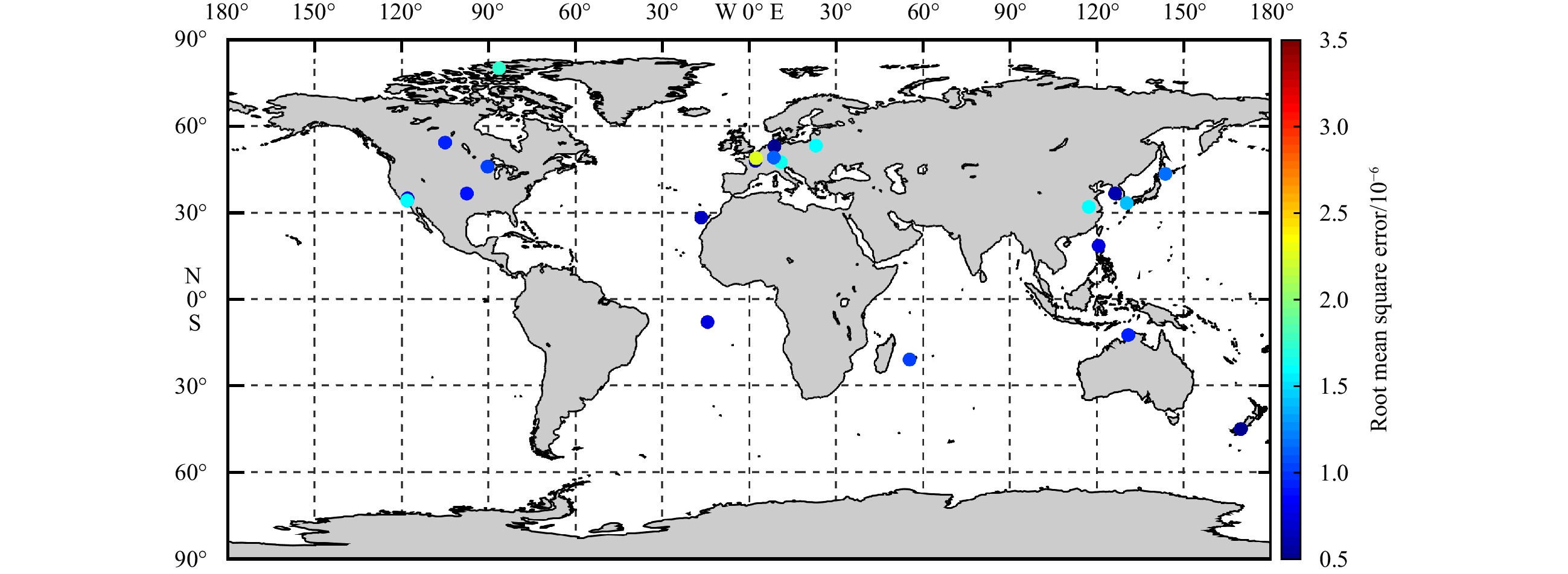
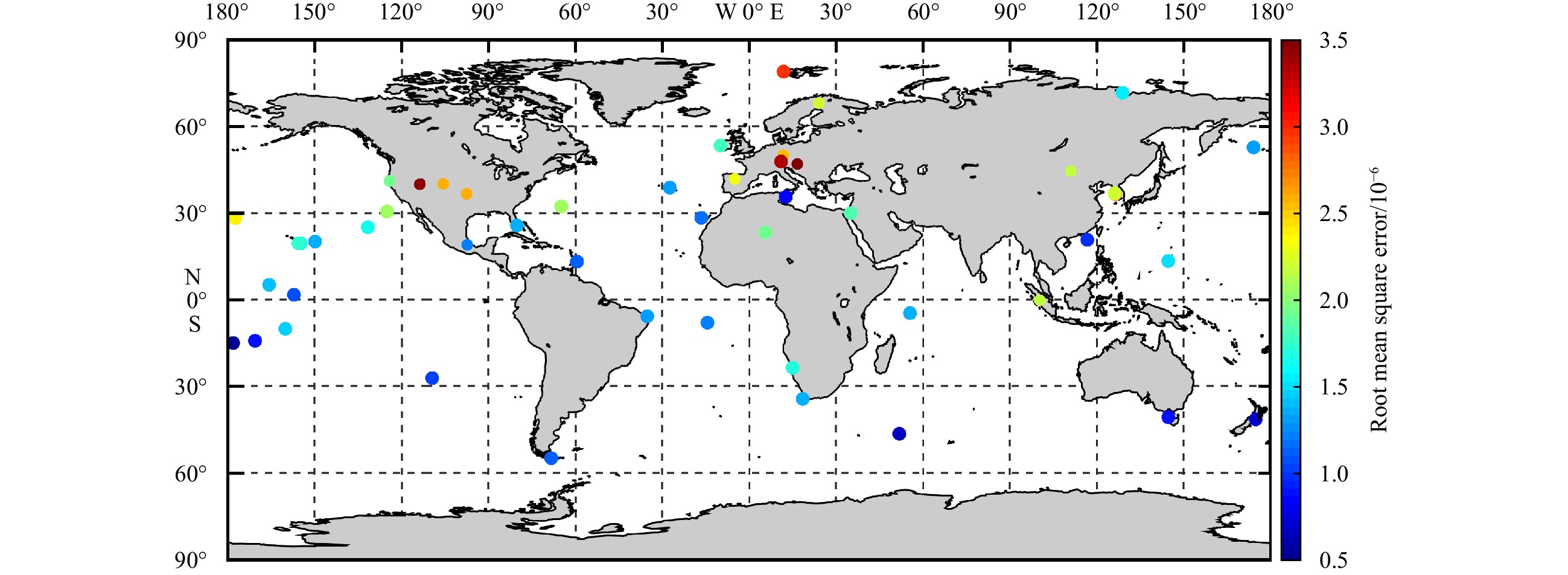
This study used ±5 h temporal windows to match OCO-2 and GMD XCO2, resulting in a time difference between OCO-2 observation and GMD measurement of less than 5 h. The distance of the matchup should also be less than 100 km. It should be noted that for cases of multiple OCO-2 XCO2 pixels matching one in situ sample, the average XCO2 value for all matchup pixels was used for further comparison. Figure 2 shows the distributions of GMD stations with matchups to OCO-2 XCO2 data. Overall, the matchup stations cover different regions of both global land and ocean, except the Antarctic.

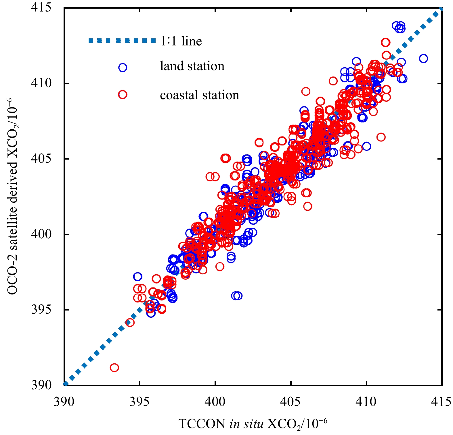
Compared to the TCCON-measured XCO2, the OCO-2 retrieved XCO2 showed a mean absolute difference of 0.247×10⁻⁶, RMSE of 1.141×10⁻⁶, and correlation coefficient (R) of 0.958 for all matchups in global ocean and land, indicating good performance of the OCO-2-retrieved XCO2 product (Fig. 3). Moreover, the OCO-2 retrieved XCO2 showed better performance in the ocean (compared with TCCON coastal sites) than it in the land (compared with TCCON terrestrial sites), as shown in Fig. 4. Specifically, for the coastal sites, the mean absolute difference is 0.121×10⁻⁶ with RMSE of 1.035×10⁻⁶ and R of 0.965, while it is 0.412×10⁻⁶ with RMSE of 1.244×10⁻⁶ and R of 0.953 for land sites. Therefore, it is obvious that OCO-2 XCO2 product has better consistency between satellite retrieval and in situ data in the oceanic region, which is expected to be related to the different retrieval algorithm and complexity of underlying surface.


Based on TCCON-measured data from 2014 to 2016, Wunch et al. (2017) found OCO-2 XCO2 was consistent with global TCCON XCO2 from September 2014 to April 2016, with a median difference of less than 0.5×10⁻⁶, RMSE typically below 1.5×10⁻⁶, and R of 0.911. Liang et al. (2017) also reported an overall bias between OCO-2 and TCCON XCO2 of (0.267 1±1.56)×10–6 from September 2014 to December 2016, with R of 0.879. Overall, our validation results are consistent with those of previous studies, and the slight differences are likely caused by the extended period of TCCON XCO2 from 2015 to 2018 in this study.
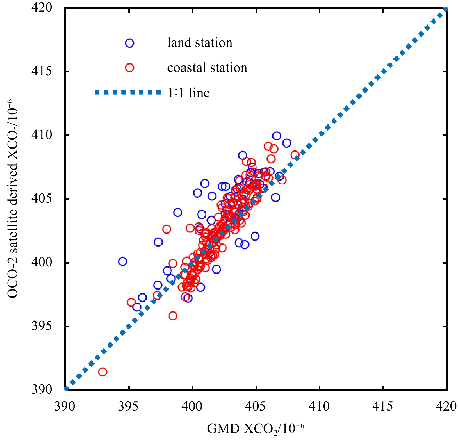
Figure 5 presents the comparisons between the OCO-2 and GMD XCO2 values. Clearly, OCO-2 XCO2 demonstrated good performance compared with GMD XCO2, with a mean absolute difference of 0.672×10⁻⁶, RMSE of 1.684×10⁻⁶, and R of 0.865. This accuracy is comparable to the validation results between the Greenhouse Gases Observing Satellite (GOSAT) and TCCON-measured XCO2, with a mean absolute difference of less than 0.4×10⁻⁶ (Maki et al., 2010) when considering the discrepancy between mean and mean absolute differences.

Similar to the comparison result with the TCCON XCO2, OCO-2 XCO2 product showed better performance over ocean (mean absolute difference of 0.441×10⁻⁶, RMSE of 1.306×10⁻⁶, and R of 0.924) than over land (mean absolute difference of 1.372×10⁻⁶, RMSE of 2.474×10⁻⁶, and R of 0.776) as comparing with the GMD data (Fig. 6). The discrepancy between OCO-2 and GMD XCO2 values reached 5×10⁻⁶ at some GMD stations on the land. This large discrepancy was likely due to the following reasons. First, there are several GMD stations located in complex terrains with significant spatial variability in topography or ground cover. Therefore, the low spatial resolution of the OCO-2 XCO2 product and the matchup windows with100 km for space and ±5 h for time may not be suitable for these stations. Although using stricter matchup windows could result in better performance, the number of effective matchups would also be reduced, making it difficult to achieve a representative assessment. Second, the modeling profiles and in-situ data to the OCO-2 XCO2 observation space were mapped to estimate GMD XCO2, which may contain some uncertainty.

It should be noted that OCO-2-retrieved XCO2 exhibited slight overestimation at low XCO2 and underestimation at high XCO2 compared to the GMD XCO2. This effect is likely caused by the different spatial resolutions between OCO-2 and GMD measurements, since OCO-2 XCO2 is the averaged value of 2.25 km×1.29 km, while GMD XCO2 is obtained at a specific site.
Although the matchup stations might be not large enough for the global distribution which comes from two reasons. The one is limited of XCO2 ground-based sites, and they are mainly distributed in developed regions (usually densely populated areas). The other reason is that the satellite is along-track observation causing the low spatial resolution of the XCO2 products.
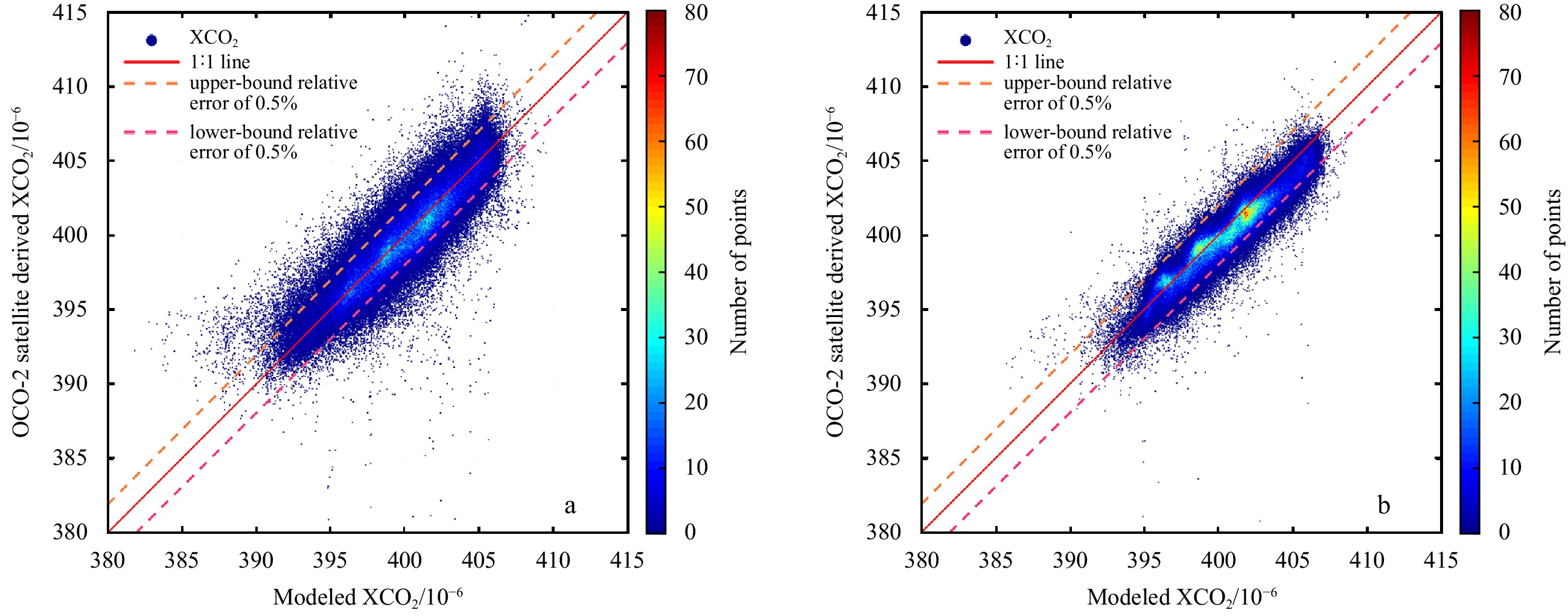
Figures 7a and b show comparisons between OCO-2-retrieved and CarbonTracker-modeled XCO2 values over land and ocean, respectively. In general, the CarbonTracker modeling results were consistent with the OCO-2-retrieved XCO2, with R of 0.897 for land and 0.945 for ocean. Thus, the CarbonTracker XCO2 product showed better performance over the ocean (mean absolute difference of 0.779×10⁻⁶, RMSE of 0.990×10⁻⁶) than over land (mean absolute difference of 1.023×10⁻⁶, RMSE of 1.399×10⁻⁶). The relatively larger discrepancy between CarbonTracker modeling and OCO-2 XCO2 over land was expected to be caused by higher inhomogeneity of XCO2 over land than over ocean. The spatial resolution of the CarbonTracker-modeled XCO2 is rather coarse (3° in longitude and 2° in latitude). In oceanic regions, XCO2 is relatively spatially uniform, and the effect of coarse resolution on the matchup between CarbonTracker-modeled and OCO-2-obtained XCO2 is therefore limited. However, over land regions, especially with high spatial inhomogeneity, the effect of coarse resolution could be significant, which might result in relatively low agreement between CarbonTracker and OCO-2 XCO2. To quantitatively analyze the differences between OCO-2 and CarbonTracker XCO2, their differences, i.e., d-XCO2 (d-XCO2=XCO2(CarbonTracker)–XCO2(OCO-2)), were determined from 2015 to 2018. Overall, d-XCO2 demonstrated near Gaussian distribution, with a mean value of –0.37×10⁻⁶ and standard deviation of 1.04×10⁻⁶. If the matchups between two datasets were divided into two groups according to the underlying surface type (land or ocean), the mean d-XCO2 for ocean was –0.17×10⁻⁶ (standard deviation of 0.93×10⁻⁶) and for land was –0.47×10⁻⁶ (standard deviation of 1.18×10⁻⁶).

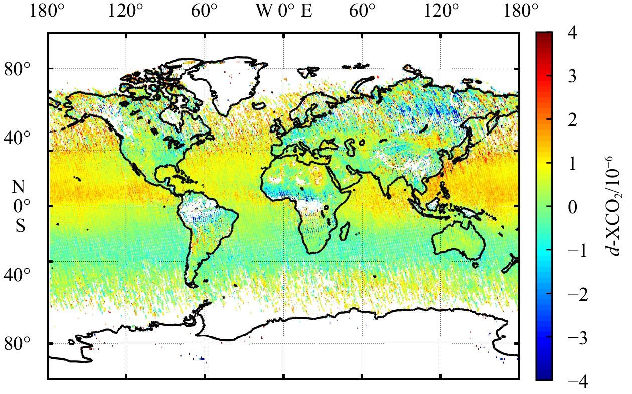
Figure 8 showed the spatial distribution of d-XCO2 at the global scale. Clearly, d-XCO2 over ocean regions demonstrated obviously discrepancies between the Northern Hemisphere (NH) and Southern Hemisphere (SH). Overall, oceanic d-XCO2 was higher in the NH than in the SH. When taking OCO-2 XCO2 as a reference, the CarbonTracker-modeled XCO2 in the NH exhibited slight underestimation over ocean regions and slight overestimation over land regions, especially in central Asia and equatorial areas. However, in the SH, the CarbonTracker XCO2 demonstrated slight overestimation over ocean regions, except at high latitudes. If 0.3% of all points, which have the largest absolute value of d-XCO2, were extract, the underestimation of XCO2 by CarbonTracker occurred more frequently in the mid- and low-latitude areas in the NH, especially oceanic regions, whereas the overestimation of XCO2 by CarbonTracker occurred more often over land regions. Northcott et al. (2019) also found greatly enhanced atmospheric CO2 levels relative to well-mixed marine atmosphere were observed during periods of offshore winds at coastal sensor platforms, which could not be exhibited by CarbonTracker.

Interestingly, there is a clear boundary for the d-XCO2 in the ocean and the land. CarbonTracker uses an offline atmospheric transport model and four surface flux modules representing four crucial CO2 transmissions. The 4-D results are interpolated for the times and locations where atmospheric observations exist, and initial net surface fluxes are adjusted using a set of weekly and regional flux scaling factors to minimize differences between the forecasted and observed CO2 mole fractions using an ensemble Kalman filter optimization scheme with a five week lag (Williams et al., 2014). This model has certain deviations in the simulation of different underlying surfaces, and the significant gap between land and ocean does not appear to be due to a faulty gas transport model and coarse spatial resolution. These deviations are more likely from incorrect estimation of input parameters (like net ecosystem exchange) to the four surface flux modules, especially a priori net ocean surface fluxes. Although large oceanic fluxes are observed in tropical and extra-tropical oceanic regions, these values are one order of magnitude smaller than that of bio-flux emissions (Maki et al., 2010). Of course, the coarse spatial resolution of CarbonTracker may also be a possible reason why the model was unsatisfactory in simulating extreme values. In addition, the differences in the representative heights of the satellite-measured and modeled XCO2 could induce variance between them. This effect could partly explain the underestimation and overestimation of the modeled XCO2 over the ocean and land areas of the NH, respectively. In the ocean regions, the glint model adopted by the satellite measurement will enhance the weight of low atmosphere layers with high CO2, which could result in higher XCO2 by satellite measurement. In contrast, the nadir model by satellite measurement over land will enhance the weight of upper atmosphere layers with low CO2, resulting in lower XCO2 by satellite measurement.
To determine the differences in temporal variations between OCO-2 and CarbonTracker XCO2, the monthly average values were calculated over 2015–2018 in low-moderate latitude areas (0°–45°) in the SH and NH, respectively (Fig. 9). Overall, the CarbonTracker-modeled XCO2 exhibited systematically higher values than the OCO-2-derived XCO2 in the NH, and the differences increased from 0.61×10⁻⁶ in 2015 to 1.28×10⁻⁶ in 2018, and an increase in the amplitude of seasonal XCO2 change could be found in the high latitude areas of the NH. Some of the previously studies pointed out that these trend are primarily driven by forest expansion and increased natural vegetation growth (Forkel et al., 2016; Graven et al., 2013), while others suggested that agricultural expansion and intensification result in increased productivity and thus enhance the seasonal variations in cultivated areas at mid-latitude regions (Gray et al., 2014; Zeng et al., 2014). In the SH, the modeled data showed smaller seasonal fluctuations than the OCO-2 XCO2 data. The SH is not considered as the main emission area of CO2, so it is also significance to consider the impact of different seasonal atmospheric circulation on the XCO2 variation (Grise and Polvani, 2017). In particular, the overestimation of the modeled data showed remarkably increase from the middle of 2016 in the SH, especially in February (0.34×10⁻⁶ in February 2015, 0.69×10⁻⁶ in February 2016, 1.34×10⁻⁶ in February 2017, 1.32×10⁻⁶ in February 2018). By analyzing the February data in 2017–2018, the largest discrepancy between the modeled and OCO-2-derived XCO2 mainly occurred in the Sahara Desert, which might be induced by uncertainty in biological flux (Williams et al., 2014).

This study compared the OCO-2 XCO2 product with in situ data from TCCON and GMD measurements and with CarbonTracker modeling. OCO-2 XCO2 was consistent with TCCON-measured XCO2, with a mean absolute difference of 0.247×10⁻⁶ and RMSE of 1.141×10⁻⁶. Compared with the GMD-derived XCO2, the OCO-2-retrieved XCO2 had a mean absolute difference of 0.672×10⁻⁶ and RMSE of 1.684×10⁻⁶. These high agreements showed that the OCO-2 could provide high quality XCO2 data over the low-moderate latitude regions. Moreover, the comparison between satellite and moldering product showed that they were relatively consistent with each other, with a mean absolute difference of 1.02×10⁻⁶ over land and 0.78×10⁻⁶ over ocean. In addition, the comparison results showed that the agreement among three different types dataset of XCO2 was higher in the oceanic area than it in the terrestrial area, indicating the high applicable of the OCO-2-retrieved XCO2 product to estimate the air-sea CO2 flux over ocean. Our results also evidenced the reliable of the CarbonTracker modeling XCO2 data, and with the advantage of the global coverage, this modeling data can also be used to estimate the air-sea CO2 flux over ocean when satellite product is unavailable.
We thank NASA for providing the OCO-2 XCO2 product, Caltech Library Research Data Repository for providing TCCON XCO2 data, and NOAA ESRL, Boulder, Colorado, USA for providing the GMD in situ data and CarbonTracker modeling data. We thank the satellite ground station, satellite data processing and sharing center, and marine satellite data online analysis platform (SatCO2) of SOED/SIO/MNR for help with data collection and processing.
| [1] |
Bai Yan, Cai Weijun, He Xianqiang, et al. 2015. A mechanistic semi-analytical method for remotely sensing sea surface pCO2 in river-dominated coastal oceans: A case study from the East China Sea. Journal of Geophysical Research: Oceans, 120(3): 2331–2349. doi: 10.1002/2014JC010632
|
| [2] |
Blumenstock T, Hase F, Schneider M, et al. 2014. TCCON data from Izana (ES), Release GGG2014R0. https://data.caltech.edu/records/293 [2017-09-13/2018-04-19]
|
| [3] |
Boesch H, Baker D, Connor B, et al. 2011. Global characterization of CO2 column retrievals from shortwave-infrared satellite observations of the Orbiting Carbon Observatory-2 mission. Remote Sensing, 3(2): 270–304. doi: 10.3390/rs3020270
|
| [4] |
Boesch H, Brown L, Castano R, et al. 2015. Orbiting Carbon Observatory (OCO)-2. https://docserver.gesdisc.eosdis.nasa.gov/public/project/OCO/OCO2_L2_ATBD.V6.pdf [2018-01-21/2018-09-16]
|
| [5] |
Bousquet P, Ciais P, Miller J, et al. 2006. Contribution of anthropogenic and natural sources to atmospheric methane variability. Nature, 443(7110): 439–443. doi: 10.1038/nature05132
|
| [6] |
Bovensmann H, Burrows J P, Buchwitz M, et al. 1999. SCIAMACHY: Mission objectives and measurement modes. Journal of the Atmospheric Sciences, 56(2): 127–150. doi: 10.1175/1520-0469(1999)056<0127:SMOAMM>2.0.CO;2
|
| [7] |
Buchwitz M, Schneising O, Burrows J P, et al. 2007. First direct observation of the atmospheric CO2 year-to-year increase from space. Atmospheric Chemistry and Physics, 7(16): 4249–4256. doi: 10.5194/acp-7-4249-2007
|
| [8] |
Cogan A J, Boesch H, Parker R J, et al. 2012. Atmospheric carbon dioxide retrieved from the Greenhouse gases observing satellite (GOSAT): Comparison with ground-based TCCON observations and GEOS-Chem model calculations. Journal of Geophysical Research: Atmospheres, 117(D21): D21301
|
| [9] |
Connor B J, Boesch H, Toon G, et al. 2008. Orbiting Carbon Observatory: Inverse method and prospective error analysis. Journal of Geophysical Research: Atmospheres, 113(D5): D05305
|
| [10] |
Crisp D. 2015. Measuring atmospheric carbon dioxide from space with the orbiting carbon observatory-2(OCO-2). In: Proceedings of SPIE 9607, Earth Observing Systems XX. San Diego, United States: SPIE, 960702
|
| [11] |
De Mazière M, Sha M K, Desmet F, et al. 2017. TCCON data from Réunion Island (RE), Release GGG2014. R1. https://data.caltech.edu/records/293 [2017-09-13/2018-04-19]
|
| [12] |
Dlugokencky E, Mund J W, Crotwell A M, et al. 2019. Atmospheric Carbon Dioxide Dry Air Mole Fractions from the NOAA ESRL Carbon Cycle Cooperative Global Air Sampling Network, 1968–2018. Boulder, USA: NOAA ESRL Global Monitoring Division
|
| [13] |
Eldering A, O'Dell C W, Wennberg P O, et al. 2017. The Orbiting Carbon Observatory 2: First 18 months of science data products. Atmospheric Measurement Techniques, 10(2): 549–563. doi: 10.5194/amt-10-549-2017
|
| [14] |
Forkel M, Carvalhais N, Rödenbeck C, et al. 2016. Enhanced seasonal CO2 exchange caused by amplified plant productivity in northern ecosystems. Science, 351(6274): 696–699. doi: 10.1126/science.aac4971
|
| [15] |
Graven H D, Keeling R F, Piper S C, et al. 2013. Enhanced seasonal exchange of CO2 by northern ecosystems since 1960. Science, 341(6150): 1085–1089. doi: 10.1126/science.1239207
|
| [16] |
Gray J M, Frolking S, Kort E A, et al. 2014. Direct human influence on atmospheric CO2 seasonality from increased cropland productivity. Nature, 515(7527): 398–401. doi: 10.1038/nature13957
|
| [17] |
Griffith D W T, Deutscher N M, Velazco V A, et al. 2014a. TCCON data from Darwin (AU), Release GGG2014R0. https://data.caltech.edu/records/293 [2017-09-13/2018-04-19]
|
| [18] |
Griffith D W T, Velazco V A, Deutscher N M, et al. 2014b. TCCON data from Wollongong (AU), Release GGG2014R0. https://data.caltech.edu/records/293 [2017-09-13/2018-04-19]
|
| [19] |
Grise K M, Polvani L M. 2017. Understanding the time scales of the tropospheric circulation response to abrupt CO2 forcing in the Southern Hemisphere: seasonality and the role of the stratosphere. Journal of Climate, 30(21): 8497–8515. doi: 10.1175/JCLI-D-16-0849.1
|
| [20] |
Hase F, Blumenstock T, Dohe S, et al. 2017. TCCON data from Karlsruhe (DE), Release GGG2014R1. https://data.caltech.edu/records/293 [2017-09-13/2018-04-19]
|
| [21] |
Intergovernmental Panel on Climate Change. 2007. Climate Change 2007: the Physical Science Basis: Working Group I Contribution to the Fourth Assessment Report of the IPCC. Cambridge: Cambridge University Press, 847–940
|
| [22] |
IPCC. 2013. Climate Change 2013: The Physical Science Basis. Working Group I Contribution to the Fifth Assessment Report of the Intergovernmental Panel on Climate Change. Cambridge: Cambridge University Press
|
| [23] |
Iraci L T, Podolske J, Hillyard P W, et al. 2016a. TCCON data from Edwards (US), Release GGG2014R1, Pasadena, California. https://data.caltech.edu/records/293 [2017-09-13/2018-04-19]
|
| [24] |
Iraci L T, Podolske J, Hillyard P W, et al. 2016b. TCCON data from Indianapolis (US), Release GGG2014R1, Pasadena, California. https://data.caltech.edu/records/293 [2017-09-13/2018-04-19]
|
| [25] |
Jacobson A R, Schuldt K N, Miller J B, et al. 2020. CarbonTracker CT2019. NOAA Earth System Research Laboratory, Global Monitoring Division. https://gml.noaa.gov/ccgg/carbontracker/CT2019/CT2019_doc.php [2018-04-19]
|
| [26] |
Jenkinson D S, Adams D E, Wild A. 1991. Model estimates of CO2 emissions from soil in response to global warming. Nature, 351(6324): 304–306. doi: 10.1038/351304a0
|
| [27] |
Joiner J, Yoshida Y, Vasilkov A, et al. 2011. First observations of global and seasonal terrestrial chlorophyll fluorescence from space. Biogeosciences, 8(3): 637–651. doi: 10.5194/bg-8-637-2011
|
| [28] |
Kawakami S, Ohyama H, Arai K, et al. 2014. TCCON data from Saga (JP), Release GGG2014R0. https://data.caltech.edu/records/293 [2017-09-13/2018-04-19]
|
| [29] |
Kivi R, Heikkinen P, Kyr. 2014. TCCON data from Sodankyla (FI), Release GGG2014R0. 637–651. https://data.caltech.edu/records/293 [2017-09-13/2018-04-19]
|
| [30] |
Liang A L, Gong W, Han G, et al. 2017. Comparison of satellite-observed XCO2 from GOSAT, OCO-2, and ground-based TCCON. Remote Sensing, 9(10): 1033. doi: 10.3390/rs9101033
|
| [31] |
Maki T, Ikegami M, Fujita T, et al. 2010. New technique to analyse global distributions of CO2 concentrations and fluxes from non-processed observational data. Tellus B, 62(5): 797–809. doi: 10.1111/j.1600-0889.2010.00488.x
|
| [32] |
Northcott D, Sevadjian J, Sancho-Gallegos D A, et al. 2019. Impacts of urban carbon dioxide emissions on sea-air flux and ocean acidification in nearshore waters. PLoS One, 14(3): e0214403. doi: 10.1371/journal.pone.0214403
|
| [33] |
Notholt J, Petri C, Warneke T, et al. 2014. TCCON data from Bremen (DE), Release GGG2014R0. https://data.caltech.edu/records/293 [2017-09-13/2018-04-19]
|
| [34] |
Notholt J, Warneke T, Petri C, et al. 2017. TCCON data from Ny Ålesund, Spitsbergen (NO), Release GGG2014. R0. https://data.caltech.edu/records/293 [2017-09-13/2018-04-19]
|
| [35] |
Peters W, Jacobson A R, Sweeney C, et al. 2007. An atmospheric perspective on North American carbon dioxide exchange: CarbonTracker. Proceedings of the National Academy of Sciences of the United States of America, 104(48): 18925–18930. doi: 10.1073/pnas.0708986104
|
| [36] |
Sherlock V, Connor B J, Robinson J, et al. 2014a. TCCON data from Lauder (NZ), 120HR, Release GGG2014R0. https://data.caltech.edu/records/293 [2017-09-13/2018-04-19]
|
| [37] |
Sherlock V, Connor B J, Robinson J, et al. 2014b. TCCON data from Lauder (NZ), 125HR, Release GGG2014R0. https://data.caltech.edu/records/293 [2017-09-13/2018-04-19]
|
| [38] |
Song Xuelian, Bai Yan, Cai Weijun, et al. 2016. Remote sensing of sea surface pCO2 in the bering sea in summer based on a Mechanistic Semi-Analytical Algorithm (MeSAA). Remote Sensing, 8(7): 558. doi: 10.3390/rs8070558
|
| [39] |
Strong K, Mendonca J, Weave D, et al. 2017. TCCON data from Eureka (CA), Release GGG2014R1. https://data.caltech.edu/records/293 [2017-09-13/2018-04-19]
|
| [40] |
Williams I N, Riley W J, Torn M S, et al. 2014. Biases in regional carbon budgets from covariation of surface fluxes and weather in transport model inversions. Atmospheric Chemistry and Physics, 14(3): 1571–1585. doi: 10.5194/acp-14-1571-2014
|
| [41] |
Wunch D, Toon G C, Blavier J F L, et al. 2011. The total carbon column observing network. Philosophical Transactions. Series A: Mathematical, Physical, and Engineering Sciences, 369(1943): 2087–2112
|
| [42] |
Wunch D, Wennberg P O, Osterman G, et al. 2017. Comparisons of the orbiting carbon observatory-2(OCO-2) XCO2 measurements with TCCON. Atmospheric Measurement Techniques, 10: 2209–2238. doi: 10.5194/amt-10-2209-2017
|
| [43] |
Yokota T, Yoshida Y, Eguchi N, et al. 2009. Global concentrations of CO2 and CH4 retrieved from GOSAT: First preliminary results. Sola, 5: 160–163. doi: 10.2151/sola.2009-041
|
| [44] |
Zeng Ning, Zhao Fang, Collatz G J, et al. 2014. Agricultural green revolution as a driver of increasing atmospheric CO2 seasonal amplitude. Nature, 515(7527): 394–397. doi: 10.1038/nature13893
|
| 1. | Hui Wang, Dan Li, Ruilin Zhou, et al. A New Method for Top-Down Inversion Estimation of Carbon Dioxide Flux Based on Deep Learning. Remote Sensing, 2024, 16(19): 3694. doi:10.3390/rs16193694 | |
| 2. | Meng Ji, Yongming Xu, Yang Zhang, et al. Validation of Remotely Sensed XCO2 Products With TCCON Observations in East Asia. IEEE Journal of Selected Topics in Applied Earth Observations and Remote Sensing, 2024, 17: 7159. doi:10.1109/JSTARS.2024.3378229 | |
| 3. | Ailin Liang, Ruonan Pang, Cheng Chen, et al. XCO2 Fusion Algorithm Based on Multi-Source Greenhouse Gas Satellites and CarbonTracker. Atmosphere, 2023, 14(9): 1335. doi:10.3390/atmos14091335 |
Figures(9)

Supported by:
Beijing Renhe Information Technology Co. Ltd

Siqi Zhang, Yan Bai, Xianqiang He, Haiqing Huang, Qiangkun Zhu, Fang Gong. Comparisons of OCO-2 satellite derived XCO2 with in situ and modeled data over global ocean[J]. Acta Oceanologica Sinica, 2021, 40(4): 136-142. doi: 10.1007/s13131-021-1844-9

 DownLoad:


 DownLoad: