Haihua Chen, Lele Li, Lei Guan. Cross-calibration of brightness temperature obtained by FY-3B/MWRI using Aqua/AMSR-E data for snow depth retrieval in the Arctic[J]. Acta Oceanologica Sinica, 2021, 40(1): 43-53. doi: 10.1007/s13131-021-1717-2
Citation:
Haihua Chen, Lele Li, Lei Guan. Cross-calibration of brightness temperature obtained by FY-3B/MWRI using Aqua/AMSR-E data for snow depth retrieval in the Arctic[J]. Acta Oceanologica Sinica, 2021, 40(1): 43-53. doi: 10.1007/s13131-021-1717-2
Haihua Chen, Lele Li, Lei Guan. Cross-calibration of brightness temperature obtained by FY-3B/MWRI using Aqua/AMSR-E data for snow depth retrieval in the Arctic[J]. Acta Oceanologica Sinica, 2021, 40(1): 43-53. doi: 10.1007/s13131-021-1717-2
Citation:
Haihua Chen, Lele Li, Lei Guan. Cross-calibration of brightness temperature obtained by FY-3B/MWRI using Aqua/AMSR-E data for snow depth retrieval in the Arctic[J]. Acta Oceanologica Sinica, 2021, 40(1): 43-53. doi: 10.1007/s13131-021-1717-2
College of Information Science and Engineering, Ocean University of China, Qingdao 266100, China
Funds:
The National Key Research and Development Program of China under contract Nos 2019YFA0607001 and 2016YFC1402704; the Global Change Research Program of China under contract No. 2015CB9539011.
This study cross-calibrated the brightness temperatures observed in the Arctic by using the FY-3B/MWRI L1 and the Aqua/AMSR-E L2A. The monthly parameters of the cross-calibration were determined and evaluated using robust linear regression. The snow depth in case of seasonal ice was calculated by using parameters of the cross-calibration of data from the MWRI Tb. The correlation coefficients of the H/V polarization among all channels Tb of the two sensors were higher than 0.97. The parameters of the monthly cross-calibration were useful for the snow depth retrieval using the MWRI. Data from the MWRI Tb were cross-calibrated to the AMSR-E baseline. Biases in the data of the two sensors were optimized to approximately 0 K through the cross-calibration, the standard deviations decreased significantly in the range of 1.32 K to 2.57 K, and the correlation coefficients were as high as 99%. An analysis of the statistical distributions of the histograms before and after cross-calibration indicated that the FY-3B/MWRI Tb data had been well calibrated. Furthermore, the results of the cross-calibration were evaluated by data on the daily average Tb at 18.7 GHz, 23.8 GHz, and 36.5 GHz (V polarization), and at 89 GHz (H/V polarization), and were applied to the snow depths retrieval in the Arctic. The parameters of monthly cross-calibration were found to be effective in terms of correcting the daily average Tb. The results of the snow depths were compared with those of the calibrated MWRI and AMSR-E products. Biases of 0.18 cm to 0.38 cm were observed in the monthly snow depths, with the standard deviations ranging from 4.19 cm to 4.80 cm.
Marginal seas play a crucial role in the global material and energy cycle (Ji et al., 2020; Tsunogai et al., 1999; Yool and Fasham, 2001). Recent studies suggest that continental marginal seas are significant contributors of terrestrial materials, such as iron (Fe) and aluminum (Al), for the open ocean through cross-shelf transport. This process may potentially enhance the primary productivity of open oceans (De et al., 2012; Middag et al., 2012;Misumi et al., 2021; Waite et al., 2016; Wang et al., 2021). The East China Sea (ECS), located between mainland China and the Ryukyu Islands, is one of the largest continental marginal seas in the northwestern Pacific Ocean. The ECS plays an important role in transporting materials from the Asian continent to the western Pacific Ocean (Liu et al., 2000; Qiao et al., 2023; Ren et al., 2015; Yuan et al., 2018).
Numerous oceanographic studies have analyzed spatial and temporal variations in the nutrients of the ECS as well as nutrient budgets for the ECS shelf, including nutrient fluxes carried by the Kuroshio incursion to the ECS shelf (Chen, 2008; Ding et al., 2019b; Gong et al., 2000; Huthnance, 1995; Yang et al., 2023; Zhang et al., 2007; Zhao and Guo, 2011). It is unclear how and where nutrients are transported across the shelf, as well as its temporal and spatial variations. Limited research has been conducted on the transportation of nutrients from the shelf to the open ocean, and there is a lack of understanding about the flux and its seasonal variations across various density layers (Liu et al., 2022b; Xu et al., 2023; Zhao and Guo, 2011). In this study, we examined the nutrient dynamics in the ECS and the nutrient exchange fluxes between the shelf water and the open ocean during the spring and summer. We aimed to enhance our understanding of the temporal and spatial variations in nutrient dynamics and the potential cross-shelf transportation of nutrients between the ECS shelf and the northwestern Pacific Ocean.
2.
Materials and methods
2.1
Sample collection
In spring, summer, and autumn of 2011 and 2013, six field observations were conducted covering the ECS (Fig. 1). In 2011, three field observations were conducted from 11 May to 7 June (spring) by the R/V Shiyan 3, from 10 to 31 August (summer) and from 17 to 29 November (autumn) by the R/V Beidou. In 2013, another three field observations were conducted from 6 to 21 May (spring) by the R/V Beidou, from 4 to 31 August (summer) by the R/V Dongfanghong 2, and from 11 October to 6 November (autumn) by the R/V Beidou. Hydrological parameters such as temperature and salinity at every station were measured using a Sea Bird 911plus CTD (conductivity-temperature-depth system). Discrete water samples were collected by 10-L Niskin bottles at depths determined by CTD readings. After collection, the water samples were filtered through pre-cleaned 0.45 μm pore-size cellulose acetate filters using a 500 mL Nalgene filtration apparatus to determine nutrient concentrations. The filtered water samples were stored in high density polyethylene bottles (Nalgene) and frozen at –20℃ until they were transported back to the laboratory for analysis.
Figure
1.
Map of the East China Sea showing sampling stations for six cruises in spring, summer, and autumn of 2011 (a) and 2013 (b). The mainly circulation regimes included the Changjiang River Diluted Water (CDW), the Taiwan Warm Current (TWC) and the Kuroshio.
The concentrations of ${{\rm {NO}}_3^-} $, ${{\rm {NO}}_2^-} $, ${{\rm {NH}}_4^+} $, ${{\rm {Si(OH)}}_4^-} $ (DSi), and ${{\rm {PO}}_4^{3-}} $ (DIP) were measured using a nutrient auto-analyzer (SkalarSANplus) (Liu et al., 2011). The concentration of dissolved inorganic nitrogen (DIN) was the sum of ${{\rm {NO}}_3^-} $, ${{\rm {NO}}_2^-} $, and ${{\rm {NH}}_4^+} $. Total dissolved nitrogen (TDN) and phosphorus (TDP) were measured using the alkaline potassium persulfate (K2S2O8) oxidation method as described by Grasshoff et al. (2009). The analytical precision was 0.06 μmol/L, 0.01 μmol/L, 0.09 μmol/L, 0.15 μmol/L, 0.03 μmol/L, 0.68 μmol/L, and 0.02 μmol/L for ${{\rm {NO}}_3^-} $, ${{\rm {NO}}_2^-} $, ${{\rm {NH}}_4^+} $, DSi, DIP, TDN and TDP, respectively. The concentrations of dissolved organic nitrogen (DON) and phosphorus (DOP) were estimated by subtracting DIN from TDN and DIP from TDP, respectively.
3.
Results
3.1
Hydrographic conditions
In the ECS, the main circulation regimes include the Kuroshio, the CDW, and the Taiwan Warm Current (TWC) (Figs 2-4) (Gong et al., 1996; Ichikawa and Chaen, 1993; Sun et al., 2023; Teague et al., 2003). The CDW, which is characterized by low salinity (S < 31), expanded southeastward to 124°E at the surface in spring. In summer, the expansion direction of CDW shifted to the northeast and covered a larger area, reaching 126.5°E near the Cheju Island. In autumn, the CDW mainly extended southward along the coast within 122.5°E. In 2011 and 2013, the seasonal changes of the CDW were similar (Figs 3 and 4).
Figure
2.
Temperature (℃) and salinity (S) diagrams of different seasons. Water masses were based on Ichikawa and Beardsley, 1993; Gong et al., 1996 and Ren et al., 2015. CDW: the Changjiang River Diluted Water; TWC: the Taiwan Warm Current; KSW: the Kuroshio Surface Water; KSSW: the Kuroshio Subsurface Water; KIW: the Kuroshio Intermediate Water; SMW: the shelf mixed water.
Figure
3.
Horizontal distribution of temperature in surface (a) and near-bottom (b) waters and salinity in surface (c) and near-bottom (d) in spring; temperature in surface (e) and near-bottom (f) and salinity in surface (g) and near-bottom (h) in summer; and temperature in surface (i) and near-bottom (j) and salinity in surface (k) and near-bottom (l) in autumn of the East China Sea.
Figure
4.
Horizontal distribution of temperature in surface (a) and near-bottom (b) waters and salinity in surface (c) and near-bottom (d) in spring; temperature in surface (e) and near-bottom (f) and salinity in surface (g) and near-bottom (h) in summer; and temperature in surface (i) and near-bottom (j) and salinity in surface (k) and near-bottom (l) in autumn of the East China Sea.
On the outer side of the ECS shelf, the influence of the Kuroshio current was dominant. The Kuroshio is one of the most powerful ocean currents in the world (Nitani, 1972). It is characterized by high salinity, originated in the North Equatorial Current System. The current flows northeast, passing through the northeastern of Taiwan Island, generally following the 200 m isobath, and ultimately deflects eastward into the Pacific Ocean through the Tokara Strait (Nitani, 1972). The Kuroshio intruded onto the ECS shelf from the northeast of Taiwan Island as it moved north (Chen, 1996; Zhou et al., 2015). The warm (T > 23℃), salty (S > 34) Kuroshio surface water (KSW) was observed along the ECS continental slope at the surface layer, and its temperature varied with the seasons (23−26℃ in spring and autumn, 25−31℃ in summer) in 2011 and 2013 (Figs 2-4).In spring 2011 and 2013, the slightly cooler (15−23℃), high salinity (>34.4) KSSW invasion occupied in the shelf edge and the middle shelf region, especially at the bottom layer, where the incursion can reach 30°N near the Changjiang River Estuary. In summer of 2011 and 2013, the temperature of KSSW increased slightly (15−25℃), and the salinity remained high. The KSSW invasion could be observed from the continental slope onto the shelf to a water depth of ca. 40 m in the near-bottom water off the Changjiang River Estuary in summer. In autumn 2013, the temperature of KSSW decreased slightly (15−23℃), and the invasion area reduced covering the continental shelf edge to the 100 m isobaths in the bottom layer. Cold (T < 15℃), salty (S > 34.2) Kuroshio Intermediate Water (KIW), was observed in spring 2011 and summer 2013 at stations located at water depths greater than 200 m. KIW appeared to be a stable water mass with no discernible seasonal variations.
The TWC originates from the Taiwan Strait and the intrusion of Kuroshio, which is characterized by relatively high temperature and low salinity (Weng and Wang, 1984; Guan, 1994). It spread over the middle and outer shelf, covering the upper water layers at a depth of 10−50 m. The salinity of the shelf mixed water (SMW) was higher than that of the CDW but lower than that of the Kuroshio. Additionally, the temperature of the SMW also lower than that of the KSW (Fig. 2).
The sea temperature varied seasonally and spatially. The surface temperature gradually increased from spring (14−24℃) to summer (22−30℃) and then decreased in autumn (18−25℃). In spring (May in 2011 and 2013), the surface temperature gradually increased from north to south and from near the shore to the outer-shelf (Fig. 2). In the summer (August in 2011 and 2013) and autumn (November in 2011 and 2013), the surface temperature gradually increased from the Changjiang River Estuary to the offshore area. High temperatures were mainly distributed over the southeast and southwest of the ECS and were strongly affected by the Kuroshio and the TWC. In different seasons, the bottom water temperature was negatively correlated with water depth, with the exception of a high value in the northern Taiwan Strait caused by the TWC. In addition, there was a low temperature water mass at the bottom layer in the north of the ECS, which was affected by the Yellow Sea Cold Water (YSCW)(Figs 3 and 4).
In both the surface and bottom layers of the ECS shelf, salinity increased from nearshore to offshore. Seawater with high salinity (S > 34) was mainly distributed in the southeast regions that were occupied by the Kuroshio, and in the southern regions that were occupied by the TWC. The surface salinity of the ECS shelf was lower in summer (August in 2011 and 2013) than in spring and autumn (November in 2011 and October in 2013) because of the greater expansion of the CDW (Figs 2-4). Salinity in the bottom water was higher in the summer, suggesting that the KSSW invasion was stronger. For stations with water depths less than 20 m near the Changjiang River Estuary, the temperature and salinity of the bottom water were similar to the temperature and salinity of surface water because of strong vertical mixing in spring (May in 2011 and 2013). In the summer, the CDW mainly spread at the surface. Significant stratification even occurred in the estuary area where the water depth is shallow; thus, the salinity of bottom water at the Changjiang River Estuary was higher (S > 31) in summer than in spring. In areas with deep water depths (especially greater than 50 m in spring and 20 m in summer and autumn), obvious stratification of the water column occurred.
3.2
Nutrients
The DIN and DSi concentrations were quite high, which is consistent with reported DIN and DSi concentrations exceeding 100 µmol/L in the Changjiang River freshwater (Dai et al., 2011; Ding et al., 2019a). The nutrient concentrations of the CDW were enriched with DIN [(27.92 ± 7.11) µmol/L for six cruises] and depleted in DIP [(0.63 ± 0.29) µmol/L] relative to the KSSW and KIW. Nutrients in the surface water of the ECS were mainly affected by the mixture of the CDW and KSW, and decreased quickly from the inner shelf (depth < 50 m) to the outer shelf (100 m < depth < 200 m) in surface water. The inorganic nutrient concentrations of KSW were the lowest, and the DIN concentration of the KSW was lower in summer than that in spring and autumn. In spring (May in 2011 and 2013), the DIN and DSi concentrations at the surface layer were higher than 5.0 µmol/L in most areas. The concentration of DIN was low (<5.0 µmol/L) only in the eastern part of the surveyed area, and the DSi concentration was low (<5.0 µmol/L) only in the southeast of the ECS, which is affected by the KSW. In most of the surface area in the ECS, DIP concentrations were lower than 0.2 μmol/L (2011) or 0.4 μmol/L (2013) (Fig. 5). In summer (August in 2011 and 2013) and autumn (November in 2011 and October in 2013), the distribution trend of dissolved inorganic nutrients (DIN, DIP and DSi) in the surface water was similar to that in spring (Figs 6 and 7). In general, the concentrations of DIN and DSi in surface seawater were lower in summer and autumn than in spring.
Figure
5.
Horizontal distribution of nutrients DIN concentration in surface (a) and near-bottom (b) waters, DIP concentration in surface (c) and near-bottom (d) waters, DSi concentration in surface (e) and near-bottom (f) waters, DON concentration in surface (g) and near-bottom (h) waters, and DOP concentration in surface (i) and near-bottom (j) waters of the East China Sea, in spring 2011.
Figure
6.
Horizontal distribution of nutrients DIN concentration in surface (a) and near-bottom (b) waters, DIP concentration in surface (c) and near-bottom (d) waters, DSi concentration in surface (e) and near-bottom (f) waters, DON concentration in surface (g) and near-bottom (h) waters, and DOP concentration in surface (i) and near-bottom (j) waters of the East China Sea, in summer 2013.
Figure
7.
Horizontal distribution of nutrients DIN concentration in surface (a) and near-bottom (b) waters, DIP concentration in surface (c) and near-bottom (d) waters, DSi concentration in surface (e) and near-bottom (f) waters, DON concentration in surface (g) and near-bottom (h) waters, and DOP concentration in surface (i) and near-bottom (j) waters of the East China Sea, in autumn 2013.
The inorganic nutrient concentrations of KSSW were relatively high, and the mean concentrations of DIN, DIP and DSi were (11.15 ± 3.99) µmol/L , (0.72 ± 0.18) µmol/L and (12.61 ± 5.39) µmol/L, respectively. The inorganic nutrient concentrations in surface water of the TWC were low and were close to those of the KSW. The inorganic nutrient concentrations in the deep water of the TWC were higher and were close to those of the KSSW. The invasion of the KSSW significantly affected the distribution of nutrients in the subsurface layer, and patterns of inorganic nutrient concentrations affected by KSSW invasion were different in different seasons. The area with high inorganic nutrient concentrations (DIN > 15.0 µmol/L, DSi > 20.0 µmol/L) in the outer shelf was smaller in summer than in spring and autumn. In spring and autumn, the area with high inorganic nutrient concentrations were caused by the invasion of KSSW, which could even extend to the middle shelf (with a water depth of ca. 50 m) of the southern ECS. This suggests that relatively few nutrients were imported into the ECS shelf because the invasion of the KSSW was low in summer. The inorganic nutrient concentrations of KIW were the highest, and the mean concentrations of these cruises were (25.42 ± 6.28) µmol/L, (1.75 ± 0.31) µmol/L and (46.36 ± 14.43) µmol/L for DIN, DIP and DSi, respectively. However, the KIW mainly existed in the slope area, and no intrusion of the KIW into the ECS shelf at water depths less than 200 m was observed in these surveys.
The vertical distributions of DIN, DSi, DIP, TDN and TDP featured high concentrations in the nearshore area (affected by the CDW) and the offshore bottom layer (affected by the KSSW)during different seasons(Figs 8 and 9). For stations at depths < 20 m near the Changjiang River Estuary, the distribution of nutrient concentrations in the water column was relatively uniform because of intense vertical mixing in spring. However, the water column began to stratify in the area at depths ≥ 50 m, leading to low concentrations of DIN, DSi and DIP in the upper layers. In summer, the vertical pattern of temperature, salinity, and nutrient concentrations was similar to that in the spring, and the difference was that stratification was more intense.
Figure
8.
Vertical distribution of temperature (a), salinity (b), σ (c) and DSi concentration (d), DIN concentration (e), DIP concentration (f), DON concentration (g) and DOP concentration (h) in PN section (depth less than 200 m), spring (May, 2011).
Figure
9.
Vertical distribution of temperature (a), salinity (b), σ (c) and DSi concentrations (d), DIN concentration (e), DIP concentration (f), DON concentration (g) and DOP concentration (h) in PN section (depth less than 200 m), summer (August, 2013).
For most of the ECS surface in spring, the concentration of DON was higher than 5 µmol/L and the concentration of DOP was higher than 0.2 µmol/L. The distribution of DON and DOP was opposite to that of dissolved inorganic nutrients. The concentrations of DON and DOP in KSW were the highest, followed by the CDW and TWC in spring. The concentrations of DON and DOP increased outwards from the Changjiang River Estuary and gradually decreased from the surface to the bottom. The DON and DOP concentrations in the three distinct water masses (KSW, KSSW, and CDW) in summer were relatively high and similar [averaged (3.77 ± 0.06) µmol/L for DON, and (0.38 ± 0.05) µmol/L for DOP]. The concentrations of DON and DOP in the KSW were slightly lower in summer than in spring, but the concentrations in the KSSW were slightly higher in summer than in spring. Areas with high concentrations of DON in summer were distributed in patches. The concentration of DON was lower than 5 µmol/L in most of the ECS surface water in summer. The DON distribution of the bottom layer was similar to that of the surface layer, but the concentrations were lower. High concentrations of DOP were observed in the middle area of the ECS shelf, and the DOP concentration was relatively high (0.6−1.2 µmol/L) from the surface to the bottom layers in summer. Although the concentrations of DON and DOP in surface water were slightly lower in summer than in spring, the high concentrations of dissolved organic nutrients could reach a depth of close to 100 m on the ECS shelf. This indicated that the influence of biological activities could reach deeper water depths in summer. The concentrations of DON and DOP were generally lower in autumn than in spring. The DOP concentrations in the surface layer gradually decreased from the Changjiang River Estuary outward, whereas DON concentrations showed the opposite pattern. This suggested that the effect of primary production and biological activities weakened in the autumn.
4.
Discussion
4.1
Nutrient composition in the ECS
In the estuary area, the influence of terrestrial input was more significant compared to other ocean regions (Jauzein et al., 2017; Wong et al., 2002). Dissolved inorganic nutrients were the primary constituents of total dissolved nutrients (TDN and TDP) in CDW. Dissolved organic nutrients were affected by various factors, such as terrestrial inputs and marine biological activities. DON accounted for 10%−20% of TDN, and DOP accounted for 30%−45% of TDP in the CDW in spring and summer of 2011 and 2013.The proportion of DON in TDN, and DOP in TDP in the CDW decreased (both below 10%) in autumn. In the KSW, DON and DOP accounted for more than 70% of TDN and TDP in the KSW over three seasons of two years, and dissolved organic nutrients were the main components of total dissolved nutrients (TDN and TDP). The primary production process and biological activities in the upper water body led to a higher content and proportion of dissolved organic nutrients (Wang et al., 2008). Dissolved inorganic nutrients were the main components of total dissolved nutrients in the KSSW. DON only accounted for 25%−29% of TDN, and DOP accounted for 13%−27% of TDP in the KSSW in spring 2011 and 2013. In the summer, DON accounted for about 30% of TDN and DOP accounted for about 40% of TDP; in autumn, the proportions decreased to around 20% for both DON and DOP in the KSSW. Similarly, dissolved inorganic nutrients were the main component of total dissolved nutrients in the TWC, and the proportion of dissolved organic nutrients being slightly higher in spring and summer (approximately 40%) than in autumn (approximately 20%). The concentration of dissolved inorganic nutrients in KSSW and TWC was higher in autumn than in spring and summer. The stratification of the water became weak, and more dissolved inorganic nutrients were replenished to the upper-middle depth water in autumn. The proportion of dissolved organic nutrients in KIW was small (<10%), and there was no obvious seasonal variation.
The DIN/DIP molar ratio in seawater has been widely used to determine nutrient structure. The DIN/DIP ratio of different water masses was different. In spring 2011, the DIN/DIP ratio of CDW was 80.7, and there was a high correlation between DIN and DIP (r = 0.75). In spring 2013, the ratio was 47.5 (r = 0.94). The DIN/DIP ratio of CDW was 58.5 (r = 0.85) in the summer of 2011, and 52.4 (r = 0.88) in the summer of 2013. However, the DIN/DIP ratio of CDW was lower in autumn than in spring and summer of 2011 and 2013. The DIN/DIP ratio of CDW was 44.2 (r = 0.83) in November 2011, and 24.6 (r = 0.94) in October 2013. The higher DIN/DIP ratio of CDW primarily stemmed from the impact of the freshwater transported from the Changjiang River into the ECS. The nutrient concentrations of the Changjiang River freshwater were enriched with DIN and depleted in DIP, which is related to anthropogenic inputs (Li et al., 2009) and the adsorption of DIP to particulate matter (Liu et al., 2009; Zhang et al., 2021). Changjiang River’s dry season runs from October to April every year, and its runoff discharge accounted for 28.9% of the annual total discharge (Tang et al., 2015). The flooding season runs from May to September and its runoff accounted for 71.1% of the annual discharge; thus, more fresh-water flows into the ECS (Tang et al., 2015). The CDW in the flooding season was more strongly affected by the freshwater discharge. This might explain why the DIN/DIP ratio of the CDW in May and August was greater. Previous studies have detected a high DIN/DIP ratio (>30) in the Changjiang River Estuary and adjacent waters in spring and summer (Wang et al., 2003; Liu et al., 2022a; Sun et al., 2023a). Other studies have also pointed out that the DIN/DIP ratio in the Changjiang River Estuary and its adjacent areas was typically between 15 and 60 in early spring (Zhou et al., 2008). Based on in-situ incubation experiments in the Changjiang River Estuary, when DIN/DIP molar ratio is greater than 30, the growth of phytoplankton is P-limited (Hu et al., 1990; Shen et al., 2008; Sun et al., 2023b). Most of the DIN/DIP ratios of the six surveys in the CDW were greater than 30 (only slightly less than 30 in the fall of 2013). Thus, the growth of phytoplankton in the CDW was P-limited. The correlation between DIN and DIP in KSW and TWC was not significant and the nutrient concentrations in most stations were low. There was obvious stratification in the water bodies in spring, summer and autumn, and the nutrients in the KSW were basically depleted. There was a relatively strong correlation between DIN and DIP (r ≥ 0.78, p < 0.01) in the KSSW and KIW, and the DIN/DIP ratio was close to the Redfield ratio. The DIN/DIP ratio in KSSW ranged from 14.3 to 14.6, and the DIN/DIP ratio of KIW ranged from 13.8 to 14.4. There was no obvious seasonal change in the DIN/DIP ratio of KSSW and KIW. In each survey, the DIN/DIP ratio of KIW was slightly lower than that of KSSW.
The invasion range of KSSW was from the shelf slope to the 50 m isobath in the near-bottom layer in spring (Figs 3d and 8b), from the shelf slope to the 40 m isobath in the near-bottom layer in summer (Figs 4h and 9b), and from the shelf slope to the 100 m isobath in the near-bottom layer in autumn (Fig. 4l). The intrusion of the KSSW not only transported a significant quantity of nutrients to the ECS shelf, but also altered the nutrient structure on the ECS shelf. The ratio of DSi and DIN was close to the Redfield ratio (≈1:1). For different water masses, the DSi/DIN molar ratios of the CDW were slightly less than 1.0, and the DSi/DIN molar ratios of KSSW, KIW and TWC were about 1.0. Generally, a non-limiting DIN and DSi supply at a DSi/DIN molar ratio large than 1 promotes the development of diatoms, which increases the abundance of zooplankton and fish, whereas lower DSi/DIN molar ratios lead to reduced zooplankton grazing (Fransz et al., 1992; Makareviciute et al., 2020) and the frequent occurrence of harmful algal blooms (Dai et al., 2011; Wang, 2006; Wang et al., 2022). There was a decrease in the riverine DSi/DIN molar ratio, from >5 in the 1960s to <1 in the 2000s (Dai et al., 2011). The DSi/DIN molar ratio in the CDW decreased to 0.85 in the 2000s (Wang, 2006). If the trend in nutrient structure change continues, the species composition of phytoplankton and ecosystem structure in the Changjiang River Estuary and its adjacent areas will change significantly, and harmful algal blooms may occur more frequently.
4.2
Nutrient storage in the euphotic zone
The euphotic layer of the sea refers to the layer where phytoplankton can photosynthesize, and this layer shows typical seasonal variations. The nutrient storage in the euphotic zone is closely related to marine primary productivity. Three surveys (spring 2011, summer 2013 and autumn 2013) with a large investigated region were selected to analyze the nutrient storage in the euphotic zone of the ECS shelf. The euphotic zone depth varied greatly in the ECS shelf. Based on the MODIS-derived results, the euphotic zone depth of the ECS shows typical seasonal variation (Shang et al., 2011). The euphotic zone depth in the high turbidity area near the Changjiang River Estuary (with water depth < 20 m and S < 31) was extremely shallow in spring, summer and autumn (<10 m). Further offshore, the euphotic zone depth of the ECS shelf was mostly 40−80 m in summer and 30−60 m in spring and autumn.
Based on the nutrient concentrations and euphotic zone depth, the nutrient storage in the euphotic zone was estimated for the ECS shelf with a surface area of 0.5 × 10⁶ km2. In spring 2011, the DIN, DIP and DSi storage in the euphotic zone was 1.37 × 10¹⁰ mol, 0.53 × 10⁹ mol, 0.84 × 10¹⁰ mol, respectively. In summer 2013, the DIN, DIP and DSi storage in the euphotic zone was 1.08 × 10¹⁰ mol, 0.89 × 10⁹ mol, 1.31 × 10¹⁰ mol, respectively. And in autumn 2013, the results were 0.75 × 10¹⁰ mol, 0.70 × 10⁹ mol, 1.09 × 10¹⁰ mol for DIN, DIP and DSi, respectively. During these surveys, the water showed obvious stratification in spring, summer and autumn, and the nutrient concentration increased with depth. On the one hand, the euphotic zone depth was deeper in summer than in spring and autumn. On the other hand, the expansion range of the CDW was large and even close to Cheju Island (Fig. 4g), and the Kuroshio water could even reach near stations with water-depth of 40 m (Figs 4h and 9b), suggesting that the effects of the CDW and the Kuroshio were more significant in the upper layer in summer and led to greater amounts of nutrients. The primary productivity of the ECS shelf was significantly higher in summer than in spring and autumn (Gong et al., 2003; Xu et al., 2022). The rich nutrient storage in the euphotic zone in summer explain the higher primary productivity.
In summer, abundant nutrients were stored in the euphotic zone, especially for DIP and DSi. The DIN/DIP ratio of the nutrient storage in the euphotic zone was closer to the Redfield ratio in summer (12.1) than that in spring (25.8) and autumn (10.7). The nutrient composition in the euphotic zone of the ECS shelf during spring indicated a trend of P-limitation. The DSi/DIN concentration ratio of the nutrient storage in the euphotic zone was lower than 1.0 in spring (0.61) and higher than 1.0 in the summer (1.21) and autumn (1.45). In spring, the nutrients reservoir in the euphotic zone had relatively low levels of DIP and DSi due to the limited amount of CDW and the exchange between shelf water and the Kuroshio. The relatively low levels of P and Si in spring was more likely to cause harmful algal blooms (Fu et al., 2012). At the beginning of the dry season (autumn), the nutrient inputs from the Changjiang River to the euphotic zone of the ECS decreased significantly. As the water temperature did not become low in autumn, phytoplankton grew vigorously and consumed large amounts of nutrients. A large amount of DIN was converted into particulate organic matter and sank below the euphotic zone. Because the cycling and regeneration of phosphate were faster than that for DIN (Lin et al., 2004; Hollister et al., 2020), the decline in the concentration of DIN in the euphotic zone was much more significant compared with DIP. This might explain why the DIN/DIP ratio was low in autumn.
4.3
Cross shelf transport of nutrients
Based on the distribution of water masses, the CDW spread outward along the surface layer, and the Kuroshio water mainly invaded the ECS shelf near the bottom layer. A nutrient plume that originated from the coast and transported outwards in the subsurface layer was detected, suggesting that there might be nutrient transport from near-shore to the open sea. For example, the cross-shelf gradient of DSi was relatively prominent in the surface layer and across the broader shelf (Fig. 10). At the bottom layer, there was a nutrient gradient from the shelf slope to the continental shelf caused by the invasion of KSSW (Figs 6 and 7). Two surveys conducted in spring 2011 and summer 2013, encompassing the entire ECS with water depths ranging from 10 m to ≥1500 m, were utilized to measure nutrient transport across the ECS shelf. The 200 m isobath was defined as the boundary between the shelf water and the Kuroshio water to study the cross-shelf transport of nutrients. Parameters such as temperature, density (σ), and DSi show strong stratification along the 200 m isobath, in which the concentrations of nutrients increased from the surface to the bottom layers along the 200 m isobaths (Fig. 11).
Figure
10.
Horizontal distributions of DSi concentration at surface layers with σ = 23.0 kg/m3 (a) and σ = 23.5 kg/m3 (b) in spring 2011; and DSi concentration (μmol/L) at surface layers with σ = 22.0 kg/m3 (c) and σ = 22.5 kg/m3 (d) in summer 2013.
Figure
11.
Vertical distribution of temperature (a), salinity (b) , σ (c) and DSi concentration (d) along 200 m isobath in spring; and temperature (e), salinity (f) , σ (g) and DSi concentration (h) along 200 m isobath in summer.
Guo et al. (2006) reported that the mean water volume transports through the 200 m isobaths was 1.46 × 10⁶ m3/s, and the surface layer showed the largest variation. Zhou et al. (2015) reported the net water flow of 1.17 × 10⁶ m3/s across the 200 m isobath. Hu et al. (2020) reported the net water flow of 1.43 × 10⁶ m3/s across the 200 m isobath. The net water exchange in the bottom layer (150 m to 200 m) was onshore, and it mostly occurred in spring and summer (Hu et al., 2020; Zhou et al., 2015). Ding et al. (2016) estimated the cross-shelf transport of sea water across the 200 m isobath in the ECS from 1993 to 2014, and the results showed that the mean flux was 1.70 × 10⁶ m3/s. The above results are relatively similar. Based on the temperature and salinity, the low-salinity CDW spread outwardly along the surface, and the KSSW invaded the ECS shelf below the surface. Because the CDW mainly expanded to the northeast in summer, except for the northern part of the ECS, the surface of other regions was strongly affected by the KSW. The expansion of low saltwater (S < 31) toward the open ocean was obvious in spring (Figs 8 and 9). These observations were basically consistent with the simulation results for the direction and trend in water transport across the 200 m isobath. Guo et al. (2006) established a high-resolution cross-shelf water exchange model, which was used to calculate the cross-shelf nutrient transport flux. The authors divided the seawater column into four layers according to depth (0−50 m, 50−100 m, 100−150 m, and 150−200 m) to study water exchange between the ECS shelf and the Kuroshio. Because the density and depth can be well matched along the 200 m isobath, the density layers corresponding to the depth layer are σ ≤ 23.0 kg/m3, 23.0 kg/m3 < σ ≤ 23.5 kg/m3, 23.5 kg/m3 < σ ≤ 24.0 kg/m3 and σ > 24.0 kg/m3 in spring, and σ ≤ 22.0 kg/m3, 22.0 kg/m 3 < σ ≤ 23.0 kg/m3, 23.0 kg/m3 < σ ≤ 23.5 kg/m3, σ > 23.5 kg/m3 in summer. Based on the water volume transports and the nutrients concentrations, the fluxes of nutrients across the 200 m isobath could be calculated (Tables 1 and 2).
Table
1.
Fluxes of water mass and nutrients across 200 m isobath on the East China Sea Shelf in spring 2011 (positive value represented invasion onto the shelf, and negative value represented transport out of shelf)
In spring, nutrients (1.16 kmol/s for DIN, 0.03 kmol/s for DIP, and 0.52 kmol/s for DSi, with the DIN/DIP molar ratio ˃ 30) in the ECS shelf transported out across the 200 m isobath through the surface layer with σ < 23.0 kg/m3, which highlighted the importance of surface cross shelf transport. Below the surface, water and nutrients entered the ESC shelf. Overall, the Kuroshio onshore flux in spring was 0.44 × 10⁶ m3/s for water volume, 8.93 kmol/s for DIN, 0.46 kmol/s for DIP, and 8.22 kmol/s for DSi. The Kuroshio subsurface water upwelling brought nutrients into the ECS shelf mainly through the bottom layer (σ > 24.0 kg/m3, depth > 150 m). The results indicated that the continental shelf water in the ECS spreads seaward in the surface layer in spring and mixes with the northwestern Pacific water, whereas the KSSW upwells and intrudes to the continental shelf mainly in the bottom layer.
In summer, water and nutrients entered the ECS shelf at four layers. The onshore flux in summer was 5.13 kmol/s for DIN, 0.41 kmol/s for DIP, and 6.42 kmol/s for DSi. The onshore flux in the surface and bottom layers accounted for 80% of the total flux. The transportation of nutrients along the surface layer to the continental shelf in summer made an important contribution to the nutrient storage and primary productivity of the euphotic zone in the ECS shelf. Although no nutrient transportation to the western Pacific Ocean through the 200 m isobath was observed in summer, part of the water with large amounts of nutrients was transported from the ECS continental shelf to the Japan/East Sea via the Tsushima Strait, which greatly affects the marine ecosystem (Chang and Isobe, 2003; Zhao and Guo, 2011).
In both spring and summer, the DIN/DIP molar ratios of onto-shelf nutrients were closed to the Redfield ratio. As mentioned above, DIP was a potential limited nutrient for phytoplankton growth in the Changjiang River Estuary and its adjacent areas. The invasion of KSSW proceeded from the shelf slope to 50 m isobaths along the near-bottom layer in spring and from the shelf slope to 40 m isobath along the near bottom layer in summer. Thus, the Kuroshio incursion not only supplied the nutrients, but also helped to alleviate the potential P-limitation in the ECS shelf area. Although the nutrient output flux through the surface only accounted for about 6% (for DSi and DIP) to 11% (for DIN) of these nutrients supplied by the Kuroshio invasion to the ECS shelf in spring, the significance of the nutrient output to the Northwest Pacific Ocean cannot be ignored. Nitrogen was the limiting element for phytoplankton growth in the Northwest Pacific (Howarth, 1988; Zhang et al., 2020). Cross-shelf transport of nutrients from shelf water to the open ocean with a relatively high DIN/DIP molar ratio (˃30) could relieve the N-limited state of the surface water in the Northwest Pacific. This might improve the primary productivity and carbon fixation of the open ocean, which has an important influence on the global carbon and nitrogen cycle. Based on the DIN flux transported out across the 200 m isobaths (1.16 kmol/s), the off-shelf transport flux of DIN throughout the spring (three months) can be estimated as 128 Gg N. The annual average atmospheric nitrogen deposition was 605 Gg/a over the Northwest Pacific Ocean (Itahashi et al., 2016). Cross shelf transport flux of DIN in spring could represent 21% of the atmospheric nitrogen deposition in the Northwest Pacific Ocean. For the Northwest Pacific Ocean, it is important to consider the effect of nutrient inputs from marginal seas on the ecosystem, as well as their temporal and spatial changes, in addition to atmospheric nitrogen deposition.
5.
Conclusions
The nutrient concentrations and their distribution in the ECS showed obvious temporal and spatial changes. In the ECS, the distribution of nutrients was significantly affected by the transportation of different water masses, such as the incursion of Kuroshio, and the CDW. Dissolved organic nutrients were affected by multiple variable, such as terrestrial inputs and marine biological activities. In the Changjiang River Estuary and its adjacent areas, DIP was a potentially limiting nutrient for phytoplankton growth during the investigated seasons. The rich-nutrients storage in the euphotic zone explained the high primary productivity in the ECS.
In spring, nutrients in coastal water were transported out across the 200 m isobath through the surface layer with σ less than 23.0 kg/m3, which highlights the importance of surface cross-shelf transport. The cross-shelf transport flux of DIN in spring was equivalent to 21% of the atmospheric nitrogen deposition in the Northwest Pacific Ocean and cross-shelf transport of nutrients to the open ocean with a relatively high DIN/DIP molar ratio (˃30). The cross-shelf nutrient transport could relieve the N-limited state of the surface water in the North Pacific. In summer, shelf water nutrient transportation across the 200 m isobath was not observed over the entire water column. Nutrient transportation from the Kuroshio to the ECS shelf primarily occurred in the surface and bottom layers, with these two layers accounting for 80% of the total flux. In both spring and summer, the DIN/DIP molar ratios of on-shelf nutrients were close to the Redfield ratio. The Kuroshio incursion not only provided nutrients but also helped alleviate potential P-limitation in the ECS shelf area.
Acknowledgements:
We greatly acknowledge the crew members of the R/V Shiyan 3, R/V Dongfanghong 2, and R/V Beidou, for their assistance, all the participants for their help and contribution during the investigation.
Abdalati W, Steffen K, Otto C, et al. 1995. Comparison of brightness temperatures from SSMI instruments on the DMSP F8 and FII satellites for Antarctica and the Greenland ice sheet. International Journal of Remote Sensing, 16(7): 1223–1229. doi: 10.1080/01431169508954473
[2]
Cavalieri D J, Comiso J, Markus T. 2014. AMSR-E/Aqua Daily L3 12.5 km Brightness Temperature, Sea Ice Concentration, & Snow Depth Polar Grids, Version 3. Boulder, Colorado USA: NASA National Snow and Ice Data Center Distributed Active Archive Center
[3]
Cavalieri D J, Parkinson C L. 2012. Arctic sea ice variability and trends, 1979–2010. The Cryosphere, 6: 881–889. doi: 10.5194/tc-6-881-2012
[4]
Cavalieri D J, Parkinson C L, DiGirolamo N, et al. 2012. Intersensor calibration between F13 SSMI and F17 SSMIS for global sea ice data records. IEEE Geoscience and Remote Sensing Letters, 9(2): 233–236. doi: 10.1109/LGRS.2011.2166754
[5]
Cavalieri D J, Parkinson C L, Vinnikov K Y. 2003. 30-year satellite record reveals contrasting Arctic and Antarctic decadal sea ice variability. Geophysical Research Letters, 30(18): 1970
[6]
Chander G, Hewison T J, Fox N, et al. 2013. Overview of intercalibration of satellite instruments. IEEE Transactions on Geoscience and Remote Sensing, 51(3): 1056–1080. doi: 10.1109/TGRS.2012.2228654
[7]
Comiso J C, Cavalieri D J, Markus T. 2003. Sea ice concentration, ice temperature, and snow depth using AMSR-E data. IEEE Transactions on Geoscience and Remote Sensing, 41(2): 243–252. doi: 10.1109/TGRS.2002.808317
[8]
Comiso J C, Parkinson C L, Gersten R, et al. 2008. Accelerated decline in the Arctic sea ice cover. Geophysical Research Letters, 35(1): L01703
[9]
Das N N, Colliander A, Chan S K, et al. 2014. Intercomparisons of brightness temperature observations over land from AMSR-E and WindSat. IEEE Transactions on Geoscience and Remote Sensing, 52(1): 452–464. doi: 10.1109/TGRS.2013.2241445
[10]
Derksen C, Walker A E. 2003. Identification of systematic bias in the cross-platform (SMMR and SSM/I) EASE-grid brightness temperature time series. IEEE Transactions on Geoscience and Remote Sensing, 41(4): 910–915. doi: 10.1109/TGRS.2003.812003
[11]
Du Jinyang, Kimball J S, Shi Jiancheng, et al. 2014. Inter-calibration of satellite passive microwave land observations from AMSR-E and AMSR2 using overlapping FY3B-MWRI sensor measurements. Remote Sensing, 6(9): 8594–8616. doi: 10.3390/rs6098594
[12]
Gao Shuo, Li Zhen, Chen Quan, et al. 2019. Inter-sensor calibration between HY-2B and AMSR2 passive microwave data in land surface and first result for snow water equivalent retrieval. Sensors, 19(22): 5023. doi: 10.3390/s19225023
[13]
Hu Tongxi, Zhao Tianjie, Shi Jiancheng, et al. 2016. Inter-calibration of AMSR-E and AMSR2 brightness temperature. Remote Sensing Technology and Application (in Chinese), 31(5): 919–924
[14]
Huang Wei, Hao Yanling, Wang Jin, et al. 2013. Brightness temperature data comparison and evaluation of FY-3B microwave radiation imager with AMSR-E. Periodical of Ocean University of China (in Chinese), 43(11): 99–111
[15]
Jezek K C, Merry C J, Cavalieri D J. 1993. Comparison of SMMR and SSM/I passive microwave data collected over Antarctica. Annals of Glaciology, 17: 131–136. doi: 10.3189/S0260305500012726
[16]
Kaleschke L, Lüpkes C, Vihma T, et al. 2001. SSM/I sea ice remote sensing for mesoscale ocean-atmosphere interaction analysis. Canadian Journal of Remote Sensing, 27(5): 526–537. doi: 10.1080/07038992.2001.10854892
[17]
Kelly R E, Chang A T, Tsang L, et al. 2003. A prototype AMSR-E global snow area and snow depth algorithm. IEEE Transactions on Geoscience and Remote Sensing, 41(2): 230–242. doi: 10.1109/TGRS.2003.809118
[18]
Li Lele, Chen Haihua, Guan Lei. 2019. Retrieval of snow depth on sea ice in the arctic using the FengYun-3B microwave radiation imager. Journal of Ocean University of China, 18(3): 580–588. doi: 10.1007/s11802-019-3873-y
[19]
Li Qin, Zhong Ruofei. 2011. Multiple surface parameters retrieval of simulated AMSR-E data. Remote Sensing for Land and Resources (in Chinese), 23(1): 42–47
[20]
Liu Qingquan, Ji Qing, Pang Xiaoping, et al. 2018. Inter-calibration of passive microwave satellite brightness temperatures observed by F13 SSM/I and F17 SSMIS for the retrieval of snow depth on Arctic first-year sea ice. Remote Sensing, 10(1): 36
[21]
Lu Zhou, Stroeve J, Xu Shiming, et al. 2020. Inter-comparison of snow depth over sea ice from multiple methods. The Cryosphere Discussions, preprint, https://doi.org/10.5194/tc-2020-65
[22]
Markus T, Cavalieri D J. 1998. Snow depth distribution over sea ice in the Southern Ocean from satellite passive microwave data. In: Jeffries M O, ed. Antarctic Sea Ice: Physical Processes, Interactions and Variability. Washington, DC: American Geophysical Union, 19–40
[23]
Markus T, Cavalieri D J. 2008. AMSR-E algorithm theoretical basis document supplement: Sea ice products. Greenbelt, MD, USA: Hydrospheric and Biospheric Sciences Laboratory, NASA Goddard Space Flight Center, 1–9
[24]
Maslowski W, Kinney J C, Higgins M, et al. 2012. The future of arctic sea ice. Annual Review of Earth and Planetary Sciences, 40(1): 625–654. doi: 10.1146/annurev-earth-042711-105345
[25]
Massom R A, Harris P T, Michael K J, et al. 1998. The distribution and formative processes of latent-heat polynyas in East Antarctica. Annals of Glaciology, 27: 420–426. doi: 10.3189/1998AoG27-1-420-426
[26]
Meier W N, Khalsa S J S, Savoie M H. 2011. Intersensor calibration between F-13 SSM/I and F-17 SSMIS near-real-time sea ice estimates. IEEE Transactions on Geoscience and Remote Sensing, 49(9): 3343–3349. doi: 10.1109/TGRS.2011.2117433
[27]
Nihashi S, Ohshima K I, Tamura T, et al. 2009. Thickness and production of sea ice in the Okhotsk Sea coastal polynyas from AMSR-E. Journal of Geophysical Research, 114(C10): C10025. doi: 10.1029/2008JC005222
[28]
Parkinson C L, Cavalieri D J. 2008. Arctic sea ice variability and trends, 1979–2006. Journal of Geophysical Research: Oceans, 113(C7): C07003
[29]
Spreen G, Kaleschke L, Heygster G. 2008. Sea ice remote sensing using AMSR-E 89-GHz channels. Journal of Geophysical Research: Oceans, 113(C2): C02S03
[30]
Stroeve J, Maslanik J, Li Xiaoming. 1998. An intercomparison of DMSP F11- and F13-derived sea ice products. Remote Sensing of Environment, 64(2): 132–152. doi: 10.1016/S0034-4257(97)00174-0
[31]
Svendsen E, Kloster K, Farrelly B, et al. 1983. Norwegian remote sensing experiment: Evaluation of the nimbus 7 scanning multichannel microwave radiometer for sea ice research. Journal of Geophysical Research: Oceans, 88(C5): 2781–2791. doi: 10.1029/JC088iC05p02781
[32]
Yang Hu, Weng Fuzhong, Lv Liqing, et al. 2011. The FengYun-3 microwave radiation imager on-orbit verification. IEEE Transactions on Geoscience and Remote Sensing, 49(11): 4552–4560. doi: 10.1109/TGRS.2011.2148200
[33]
Yang Hu, Zou Xiaolei, Li Xiaoqing, et al. 2012. Environmental data records from FengYun-3B microwave radiation imager. IEEE Transactions on Geoscience and Remote Sensing, 50(12): 4986–4993. doi: 10.1109/TGRS.2012.2197003
[34]
Zhang Shugang. 2012. An algorithm to detect arctic sea ice edge using microwave brightness temperature. Periodical of Ocean University of China (in Chinese), 42(11): 1–7
Tiantian Wang, Jiangyuan Zeng, Kun-Shan Chen, et al. Comparison of Different Intercalibration Methods of Brightness Temperatures From FY-3D and AMSR2. IEEE Transactions on Geoscience and Remote Sensing, 2022, 60: 1. doi:10.1109/TGRS.2022.3176748
2.
Haihua Chen, Xin Meng, Lele Li, et al. Quality Assessment of FY-3D/MERSI-II Thermal Infrared Brightness Temperature Data from the Arctic Region: Application to Ice Surface Temperature Inversion. Remote Sensing, 2022, 14(24): 6392. doi:10.3390/rs14246392
3.
Hairui Hao, Jie Su, Qian Shi, et al. Arctic sea ice concentration retrieval using the DT-ASI algorithm based on FY-3B/MWRI data. Acta Oceanologica Sinica, 2021, 40(11): 176. doi:10.1007/s13131-021-1839-6
4.
Hui Wang, Qizhen Sun, Lin Zhang, et al. Improving the observation and prediction capabilities for Arctic marine environment: from the perspective of Arctic Shipping. Acta Oceanologica Sinica, 2021, 40(1): 1. doi:10.1007/s13131-021-1822-2
5.
Lele Li, Haihua Chen, Lei Guan. Retrieval of Snow Depth on Arctic Sea Ice from the FY3B/MWRI. Remote Sensing, 2021, 13(8): 1457. doi:10.3390/rs13081457
6.
Tianwen Feng, Xiaohua Hao, Jian Wang, et al. Quantitative Evaluation of the Soil Signal Effect on the Correlation between Sentinel-1 Cross Ratio and Snow Depth. Remote Sensing, 2021, 13(22): 4691. doi:10.3390/rs13224691
7.
Tiantian Wang, Jiangyuan Zeng, Kun-Shan Chen, et al. Intercalibration of FY-3D MWRI against AMSR2. IGARSS 2022 - 2022 IEEE International Geoscience and Remote Sensing Symposium, doi:10.1109/IGARSS46834.2022.9883941
Haihua Chen, Lele Li, Lei Guan. Cross-calibration of brightness temperature obtained by FY-3B/MWRI using Aqua/AMSR-E data for snow depth retrieval in the Arctic[J]. Acta Oceanologica Sinica, 2021, 40(1): 43-53. doi: 10.1007/s13131-021-1717-2
Haihua Chen, Lele Li, Lei Guan. Cross-calibration of brightness temperature obtained by FY-3B/MWRI using Aqua/AMSR-E data for snow depth retrieval in the Arctic[J]. Acta Oceanologica Sinica, 2021, 40(1): 43-53. doi: 10.1007/s13131-021-1717-2
Table
1.
Fluxes of water mass and nutrients across 200 m isobath on the East China Sea Shelf in spring 2011 (positive value represented invasion onto the shelf, and negative value represented transport out of shelf)
Figure 1. Cross-calibration for 10.7–89.0 GHz (H/V polarization, ascending) in January 2011.
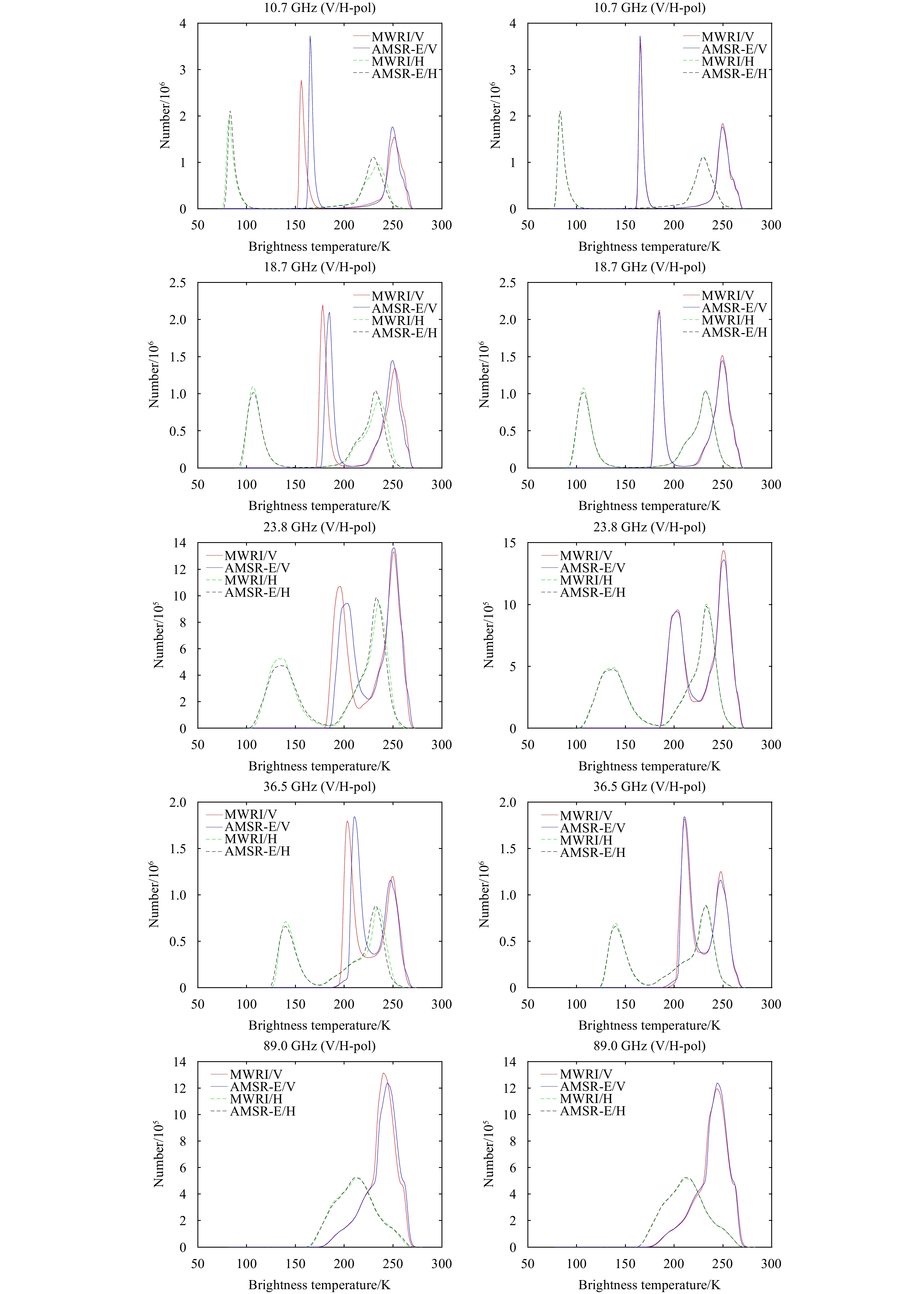
Figure 2. Statistical histograms of data on Tb of the MWRI and AMSR-E (before and after calibration) for all channels with H/V polarization (left: original MWRI and AMSR-E; right: corrected MWRI and AMSR-E).
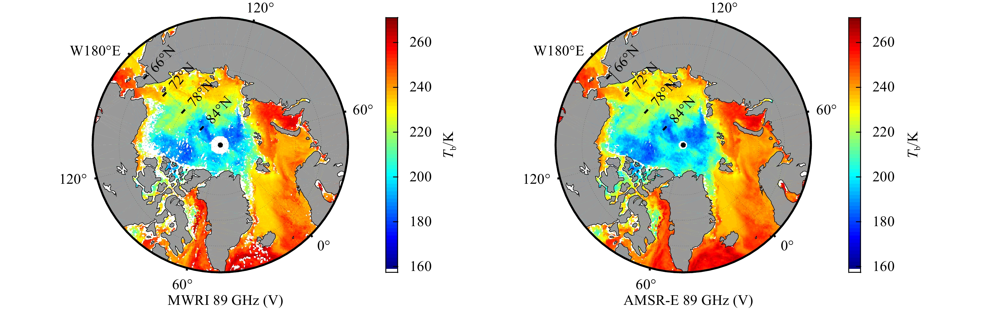
Figure 3. Comparison of daily average values of Tb for the MWRI and AMSR-E (V polarization 89 GHz, on January 1, 2011).
Figure 4. Comparison of the biases, STD, and RMSE in terms of values of Tb between the MWRI and the AMSR-E (channels: V18.7 GHz, V23.8 GHz, V36.5 GHz, H/V 89.0 GHz), before and after cross calibration.
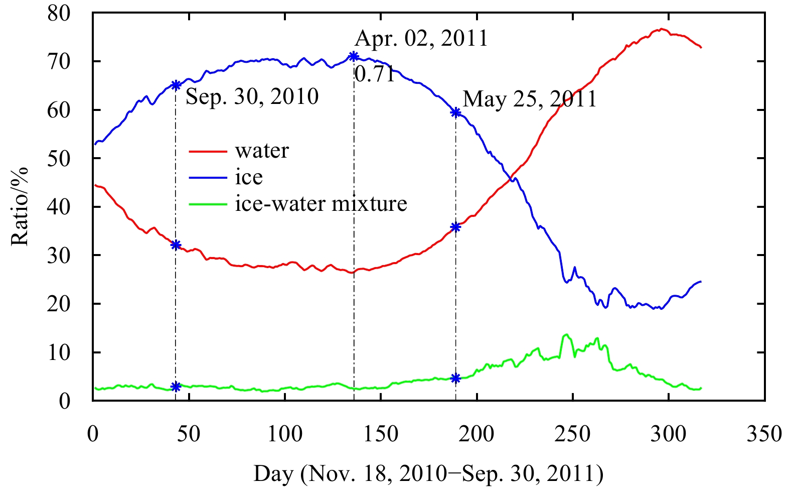
Figure 5. Ratios of the water, ice, and ice-water mixture in the Arctic.
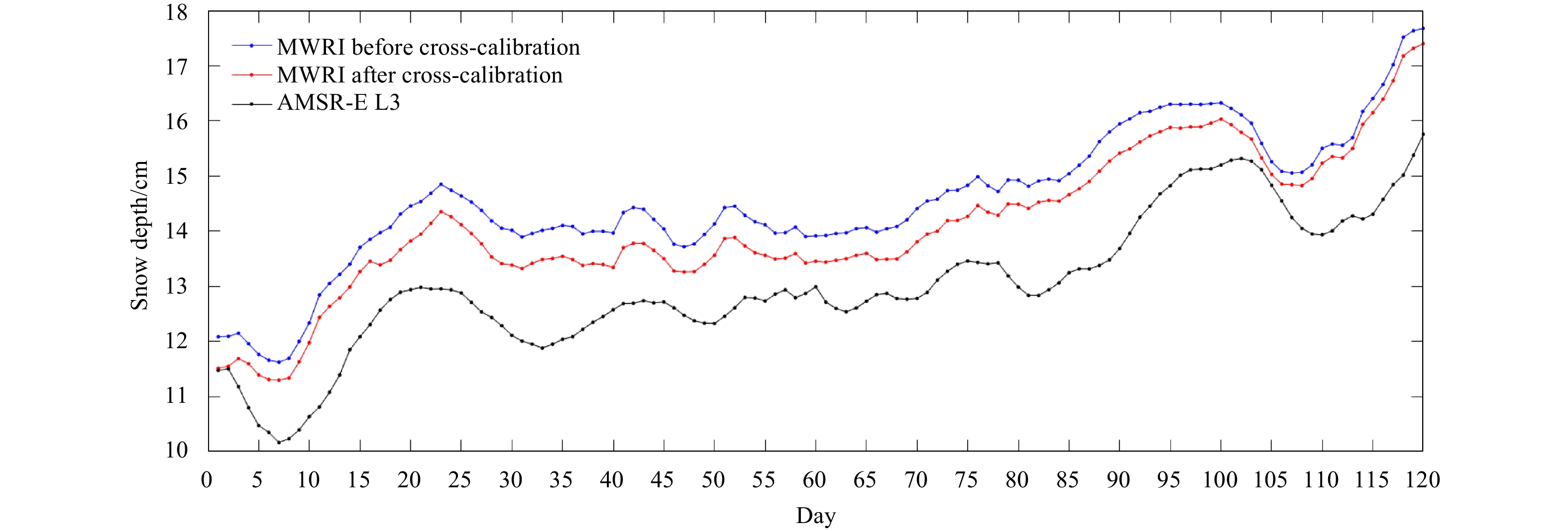
Figure 6. Comparison of distributions of snow depth derived from the MWRI before and after cross-calibration, and those of the AMSR-E level 3 in the Arctic.
Figure 7. Comparison of snow depth obtained by the MWRI and AMSR-E L3 from January 1 to April 30, 2011 (120 d).
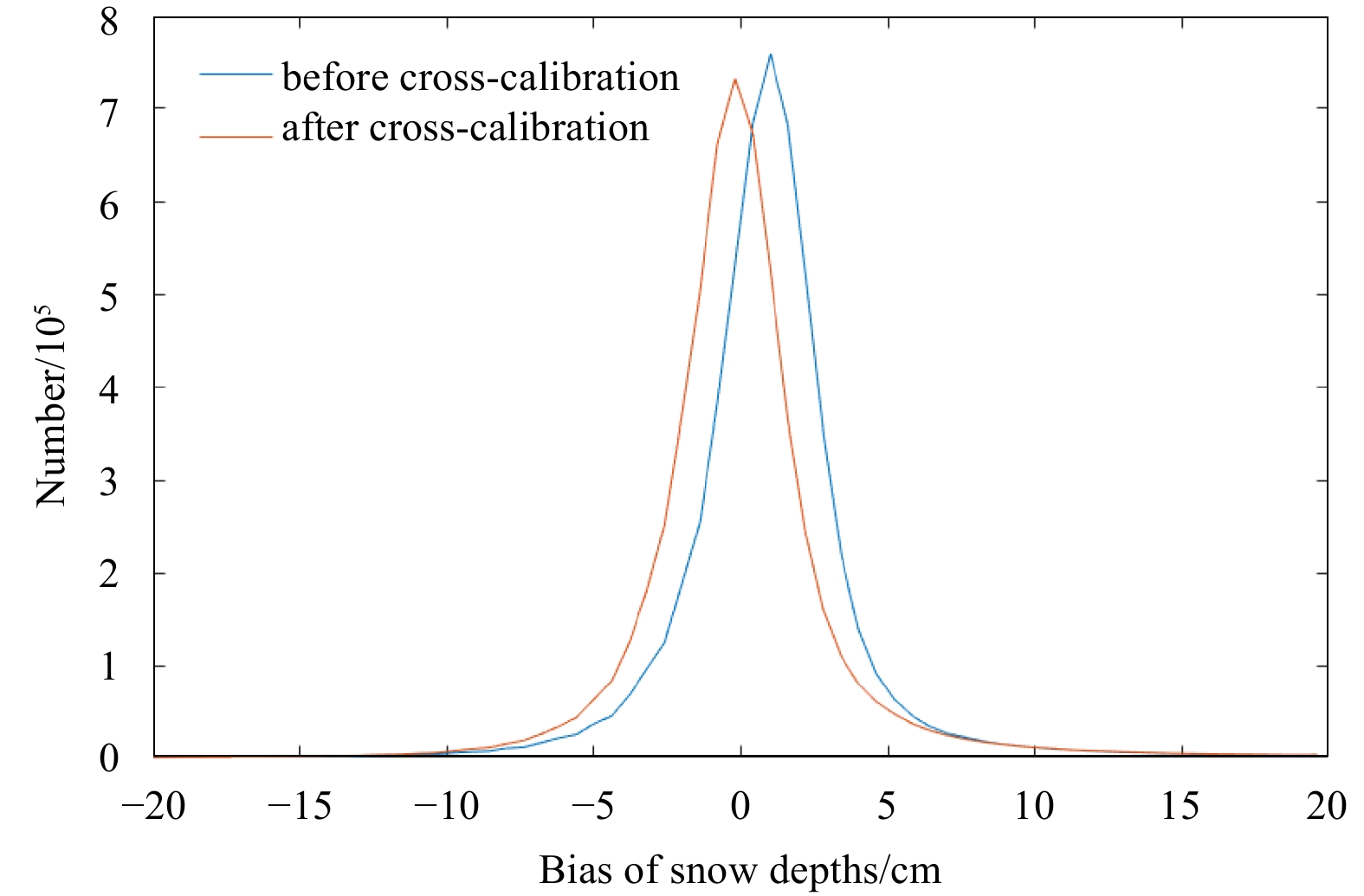
Figure 8. The histogram of snow depth biases between the MWRI (before and after cross-calibration) and AMSR-E data from January 1 to April 30, 2011
Figure 9. The Mean absolute error (MAE) of snow depths between the MWRI results and the AMSR-E L3 products from January 1 to April 30, 2011 (120 d).


 DownLoad:


 DownLoad:


 DownLoad: